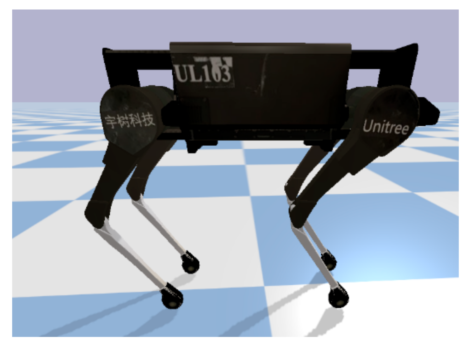
Adaptive Motion Skill Learning of Quadruped Robot on Slopes Based on Augmented Random Search Algorithm

Abstract

To deal with the problem of stable walking of quadruped robots on slopes, a gait planning algorithm framework for quadruped robots facing unknown slopes is proposed. We estimated the terrain slope by the attitude information measured by the inertial measurement unit (IMU) without relying on the robot vision. The crawl gait was adopted, and the center of gravity trajectory planning was carried out based on the stability criterion zero-moment point (ZMP). Then, the augmented random search (ARS) algorithm was used to modulate the parameters of the Bezier curve to realize the planning of the robot foot trajectory. Additionally, the robot can adjust the posture in real time to follow the desired joint angle, which realizes the adaptive adjustment of the robot’s posture during the slope movement. Simulation experiment results show that the proposed algorithm for slope gait planning can adaptively adjust the robot’s attitude and stably pass through the slope environment when the slope is unknown.

1. Introduction

The quadruped robot greatly expands the motion range of the robot thanks to the design of the robot’s bionic legs. For challenging terrains that wheeled and tracked robots cannot pass, quadruped robots have the potential to pass through. At present, it has broad development prospects and important research value in various fields, such as education, medical care, service, industry, and military [1]. However, compared with quadrupeds mammals in nature, there is still a big gap in the ability of quadruped robots to move and adjust in complex environments.

To make the quadruped robot move stably on challenging terrain, the stability of the robot is generally improved by selecting a static gait. Professor McGhee’s team [2] firstly described the static gait of the quadruped robot and realized the stable walking of the quadruped robot’s static gait. However, McGhee’s study only considers the quadruped robot on a flat road, and cannot be applied to challenging terrain. Ref. [3] planned the static gait of the quadruped robot, which can be used for the robot to walk on irregular terrain. Ref. [4] designed a quadruped robot motion controller with layered control and realized the quadruped robot’s movement on challenging terrain based on the selection of the best foothold. However, the controller needs to model the environment and has poor real-time performance. In addition, it is difficult to obtain the optimal strategy because there are a large number of parameters to be designed in the control system.

Inspired by biology, the control method based on a central pattern generator (CPG) [5] helps to improve the stability and environmental adaptability of robot motion. J.C. Montesdeoca et al. [6] used the CPG model to develop a controller capable of generating omnidirectional motion and successfully applied it to a physical robot; Ref. [7] designed a quadruped robot foot trajectory based on CPG and then used the kinematics and dynamics model to realize the robot’s movement on challenging terrain. However, the feedback is simply superimposed to the trajectories generated by the CPG, and thus the stability properties of CPGs are not exploited.

Gehring et al. [8] modeled the terrain as a plane and estimated the terrain information, and then adjusted the robot’s strategy. Additionally, they successfully achieved a dynamic trot on the slope. We adopt an overall architecture similar to that of [8]; however, in this paper, we used a reinforcement learning algorithm to train a parameterized linear policy to reduce computation.

In recent years, with the development of artificial intelligence technology and the increase in computing resources, some intelligent algorithms, such as reinforcement learning and evolutionary strategy, have become more and more popular. Nate Kohl et al. [9] first applied reinforcement learning to the field of quadruped robot motion, using a policy gradient algorithm to optimize robot foot trajectory parameters. The most classic one is policies modulating trajectory generators [10], which combines open-loop leg trajectories with neural network feedback, and the trained robot can walk stably; however, these deep-neural-network-based policies are computationally intensive and were unable to generalize to rough terrain walking. Ref. [11] incorporated proprioceptive feedback in locomotion control and trained the controller using reinforcement learning. The trained ANYmal robot can traverse various difficult terrains without explicit perception. However, the 12-layer deep neural network and the huge amount of data require expensive equipment to realize, and this work is almost non-transferable.

To deal with the problems existing in the above research, a typical environment of the slope with an unknown slope is selected, and a motion planning algorithm for quadruped robot is proposed. First, we initialized the simulation environment and used the joint angle data obtained from the robot leg motor encoder to estimate the slope of the terrain. Next, we planned the trajectory of the center of gravity to obtain the position of the next foothold, and then used the Bezier curve to generate the trajectory of the robot foot. The ARS algorithm receives data from sensors to guide the robot’s motion, allowing the robot to adaptively adjust its attitude to follow changes in the desired attitude angle. The algorithm frame is shown in Figure 1. The specific implementation of the algorithm will be described in detail in the following sections.

The main contributions of this paper can be summarized as follows:

(1)

An algorithm for estimating unknown terrain slope based on the coordinates of the foot endpoint is proposed;

(2)

We parameterized the foot end trajectory of the quadruped robot based on the Bezier curve to improve the training speed of the robot;

(3)

The ARS algorithm was used to optimize the trajectory of the foot end, and the adaptive adjustment of the robot posture is realized.

The algorithm is verified on the simulation platform, and the robot can follow the desired roll and pitch angles to achieve adaptive attitude adjustment and pass through the slope environment when the slope is unknown.

The remainder of this paper contains the following contents. Section 2 introduces robot model and terrain slope estimation algorithm. Section 3 introduces the whole control framework, including the trajectory planning of the center of gravity, the trajectory planning of the foot end, and the ARS algorithm. In Section 4, we verified the algorithm on the simulation platform and analyzed the simulation experiment results. Finally, Section 5 summarizes all the work and introduces future work.

2. Robot Model and Terrain Slope Estimation Algorithm

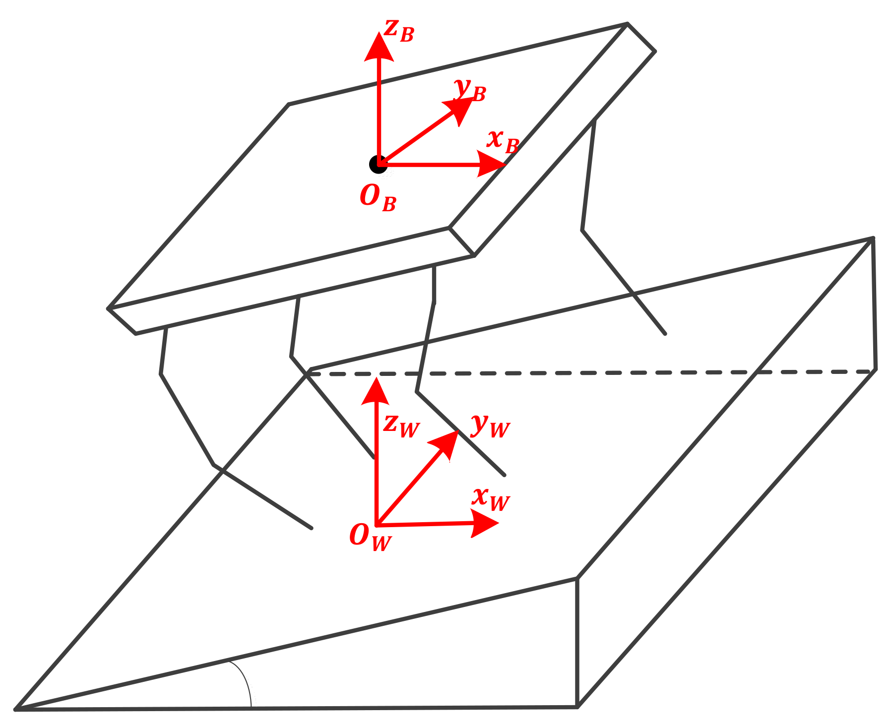
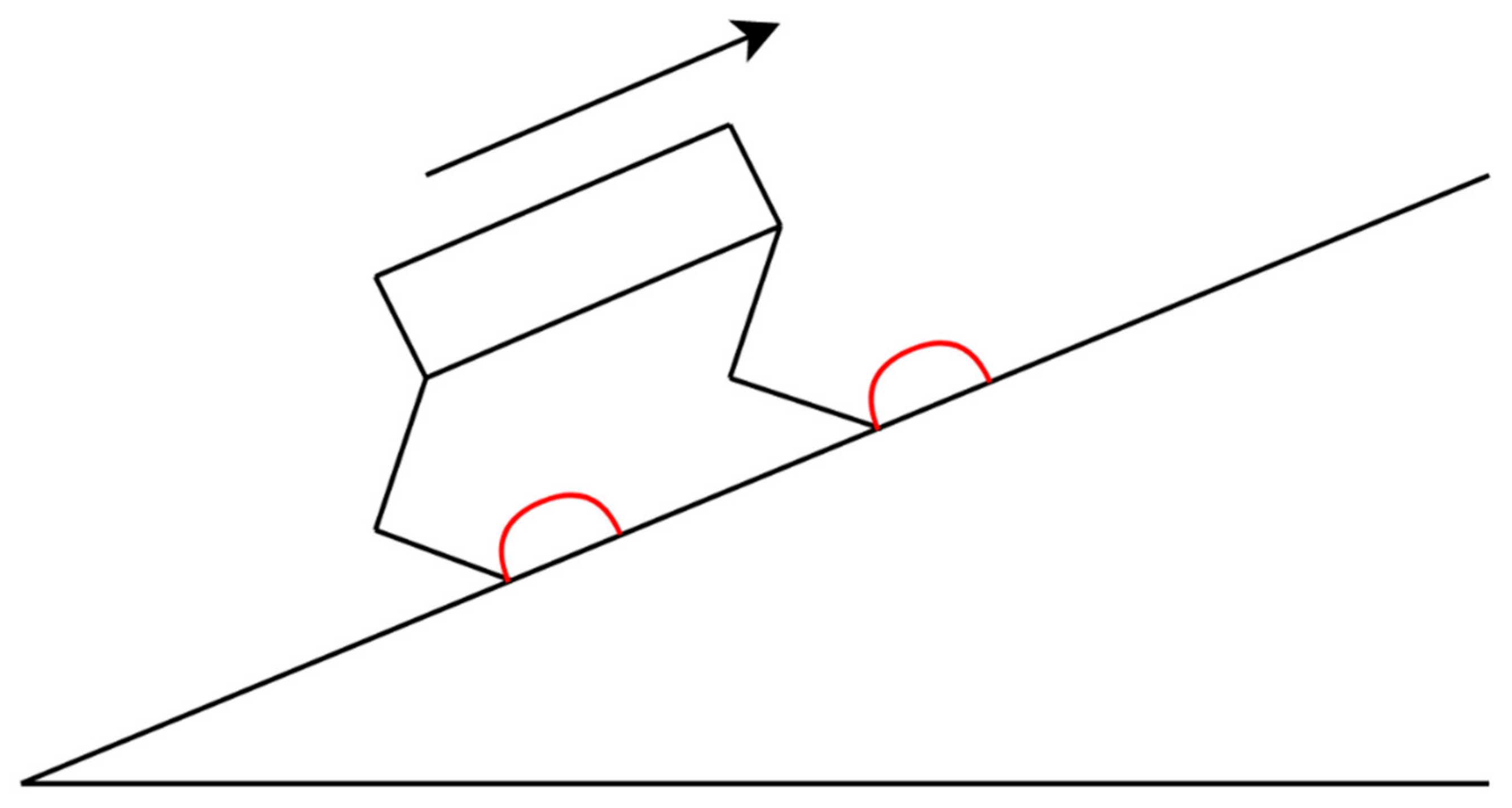
2.1. Model of a Robot on a Slope

The terrain slope is one of the important parameters to characterize the terrain information. When facing the sloped terrain, the body of the quadruped robot needs to maintain a certain posture to adapt to the sloped terrain. Generally speaking, it can be divided into a posture parallel to the ground plane or a posture parallel to the inclined plane. When the body posture is parallel to the inclined plane, the motion trend of the front and rear legs of the robot is similar, and the leg movement space of the robot leaves a margin. Therefore, this paper adopts a posture parallel to the inclined plane to move on the inclined plane.

A diagram of the quadruped robot moving on the slope is shown in Figure 2. The four legs of the robot are defined as Left Fore (LF), Right Fore (RF), Left Hide (LH), and Right Hide (RH). A single-leg coordinate system is established at the hip joint, respectively, {LFH}, {RFH}, {LHH}, and {RHH}. The world reference coordinate system, {W}, is established with the projection of the robot’s initial centroid coordinate position on the horizontal ground as the origin. The Z-axis is in the opposite direction of gravity, the X-axis points to the horizontal advance direction of the robot at the initial moment, and the Y-axis is determined by the right-hand rule. The position of the center of mass of the robot torso is defined as the body center of mass coordinate system, {B}, and the coordinate axis is parallel to the world reference coordinate system, {W}.

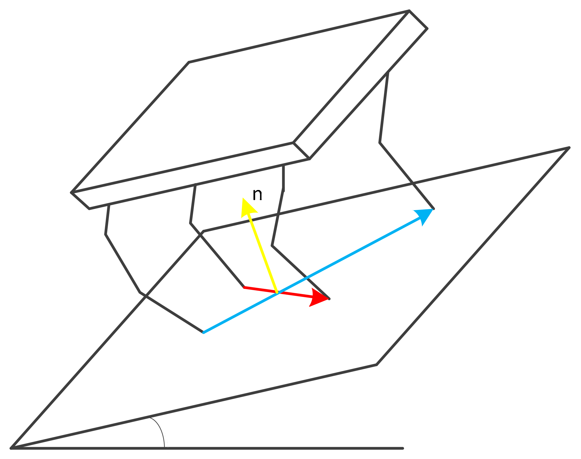
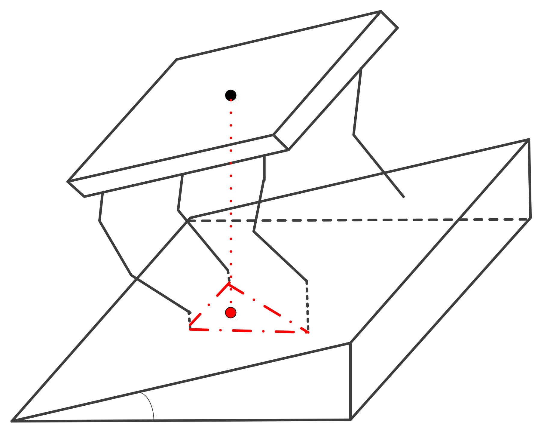
2.2. Terrain Slope Estimation

In this paper, the coordinate position of the foot end of the robot is used to estimate the terrain slope, as shown in Figure 3. Each leg of a quadruped robot has three degrees of freedom, and each degree of freedom corresponds to a motor. By reading the motor data at the robot joints, and using the robot’s forward kinematics equation, we can obtain the coordinates of the robot’s foot in the body center of mass coordinate system {B}:

$$p_i=f\left({\theta }_{r_i},{\theta }_{k_i},{\theta }_{p_i}\right)$$

(1)

where $p_i$ is the position of the foot i, where $i\in \left\{LF,LH,RF,RH\right\}$, in the body center of mass coordinate system {B}, and ${\theta }_{r_i},{\theta }_{k_i},{\theta }_{p_i}$ are the angles of the abduction, hip, and knee actuators, respectively, of the leg, i. Additionally, $f\left(\cdots \right)$ is the forward kinematics function, that is, given the angle of each joint of the robot, it calculates the coordinates of the foot end of the robot. After obtaining the coordinates of the foot end, the terrain slope can be estimated.

According to the coordinates of the robot foot point, the slope normal vector, $\overrightarrow{n}$, can be obtained:

$$\overrightarrow{n}=\left(p_1-p_3\right)\times \left(p_2-p_4\right)$$

(2)

Furthermore, we can obtain the desired pitch angle ${\theta }_P$ and roll angle ${\theta }_R$ of the robot.

$$\overrightarrow{N}=R_Y\left({\theta }_P\right)R_X\left({\theta }_R\right)\left(\begin{array}{c}0\\ 0\\ 1\end{array}\right)$$

(3)

$$\left\{\begin{array}{c}{\theta }_P=-arcsin\overrightarrow{N_y}\\ {\theta }_R=arctan\frac{\overrightarrow{N_x}}{\overrightarrow{N_z}}\end{array}\right.$$

(4)

where $\overrightarrow{N}={\left(\overrightarrow{N_x}\overrightarrow{N_y}\overrightarrow{N_z}\right)}^T$ is the unit normal vector of the slope, and $R_Y$ and $R_X$ are the rotation matrix.

$$R_X\left({\theta }_R\right)=\left(\begin{array}{ccc}1& 0& 0\\ 0& cos\left({\theta }_R\right)& -sin\left({\theta }_R\right)\\ 0& sin\left({\theta }_R\right)& cos\left({\theta }_R\right)\end{array}\right)$$

(5)

$$R_Y\left({\theta }_P\right)=\left(\begin{array}{ccc}cos\left({\theta }_P\right)& 0& sin\left({\theta }_P\right)\\ 0& 1& 0\\ -sin\left({\theta }_P\right)& 0& cos\left({\theta }_P\right)\end{array}\right)$$

(6)

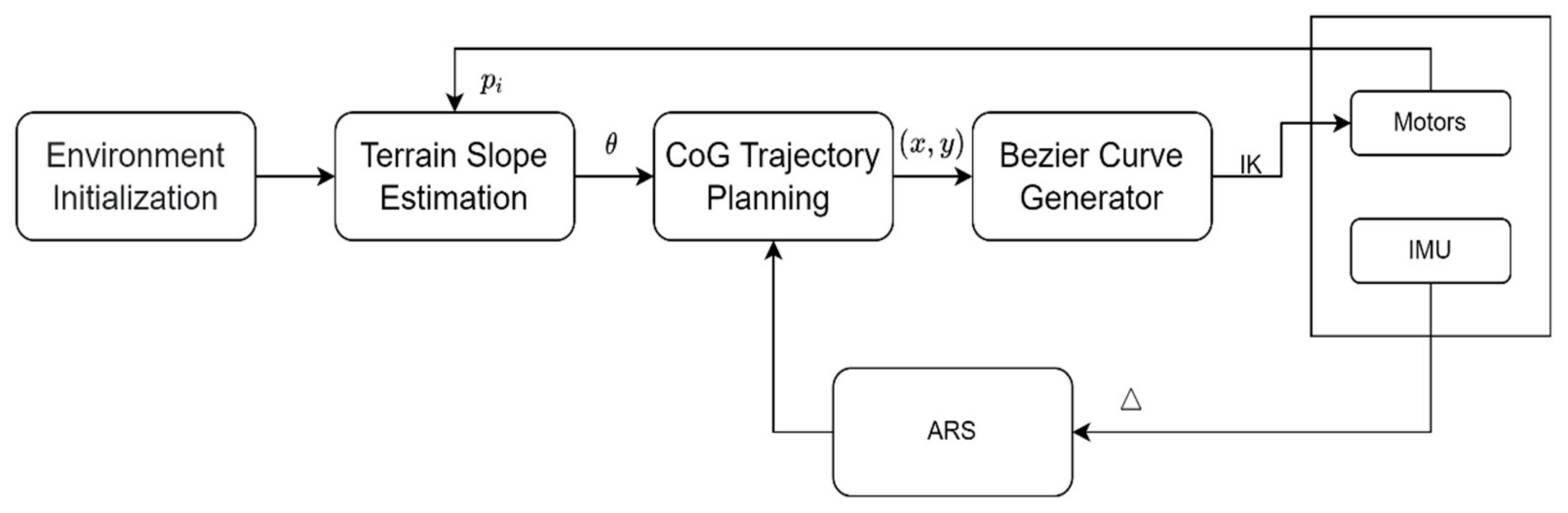
3. Control Architecture

3.1. Zero-Moment Point

In 1972, Vukobratovic first proposed the zero-moment point (ZMP) theory [12] as a dynamic stability criterion for robots. ZMP refers to a point on the ground, which the component of the resultant moment of inertial force and gravity acting on the robot in the horizontal direction of this point is 0. The research shows that, when the robot moves, if the ZMP is located in the support polygon formed by the robot’s sole and the ground, then the stability of the robot’s movement process will be guaranteed.

When the robot moves on the slope, the projection of the footfall point of the inclined plane on the horizontal plane will be reduced, so the area of the robot’s stable support triangle will be reduced. As shown in Figure 4. Additionally, the projected position of the robot’s center of gravity may fall outside the stable support triangle. Therefore, the quadruped robot should adjust the foot position to change the robot’s posture to achieve stable walking on the slope.

In this paper, the swing of the left front leg is analyzed, and the landing point of the robot on the inclined plane is projected to the world reference coordinate system, {W}. The triangle formed by the solid line is the stable support domain on the right, and the vertex of the stable support triangle is s, RH and RF. The shortest distance from ZMP to the three sides of the supporting triangle is defined as the stability margin. When the ZMP is located inside the supporting triangle, the stability margin is positive, the robot is in a stable walking state. The stability has the most maximum margin when the ZMP coincides with the center of the incircle of the supporting triangle. Assume that the projected coordinates of the three landing points of the robot in the world reference coordinate system, {W}, are $W_{LH}\left(x_{LH},y_{LH}\right)$, $W_{RH}\left(x_{RH},y_{RH}\right)$, and $W_{RF}\left(x_{RF},y_{RF}\right)$. The projected coordinates of the expected landing point of the LF leg in the world reference coordinate system, {W}, are $W_{LF}\left(x_{LF},y_{LF}\right)$. The diagram of the landing point of the quadruped robot in the world reference coordinate system, {W}, is shown in Figure 5.

First, we used the four endpoints to solve the equations of the straight line $L_{LH-RF}$ and the straight line $L_{LF-RH}c$, and then we obtained the coordinates $W_s\left(x_s,y_s\right)$ of the intersection of the two straight lines.

$$\left\{\begin{array}{c}{x}_s=\frac{b_2-b_1}{k_1-k_2}\\ y_s=k_1{x}_s+b_1\end{array}\right.$$

(7)

$$\left\{\begin{array}{c}{b}_1=y_{LF}-\frac{y_{LF}-y_{RH}}{x_{LF}-x_{RH}}{x}_{LF}\\ b_2=y_{RF}-\frac{y_{RF}-y_{LH}}{x_{RF}-x_{LH}}{x}_{RF}\end{array}\right.$$

(8)

$$\left\{\begin{array}{c}{k}_1=\frac{y_{LF}-y_{RH}}{x_{LF}-x_{RH}}\\ k_2=\frac{y_{RF}-y_{LH}}{x_{RF}-x_{LH}}\end{array}\right.$$

(9)

Therefore, according to the coordinates of the three vertices of the triangle $∆W_s{W}_{RH}{W}_{RF}$, the lengths of the three sides can be obtained as:

$$\left\{\begin{array}{c}{L}_{RH-RF}=\sqrt{{\left(x_{RH}-x_{RF}\right)}^2+{\left(y_{RH}-y_{RF}\right)}^2}\\ L_{s-RF}=\sqrt{{\left(x_s-x_{RF}\right)}^2+{\left(y_s-y_{RF}\right)}^2}\\ L_{s-RH}=\sqrt{{\left(x_s-x_{RH}\right)}^2+{\left(y_s-y_{RH}\right)}^2}\end{array}\right.$$

(10)

Furthermore, the center of the incircle of the supporting triangle can be obtained as:

$$\left\{\begin{array}{c}{x}_I=\frac{L_{RH-RF} \ast x_s+L_{s-RF} \ast x_{RH}+L_{s-RH} \ast x_{RF}}{L_{RH-RF}+L_{s-RF}+L_{s-RH}}\\ y_I=\frac{L_{RH-RF} \ast y_s+L_{s-RF} \ast y_{RH}+L_{s-RH} \ast y_{RF}}{L_{RH-RF}+L_{s-RF}+L_{s-RH}}\end{array}\right.$$

(11)

3.2. Center of Gravity Trajectory Generator

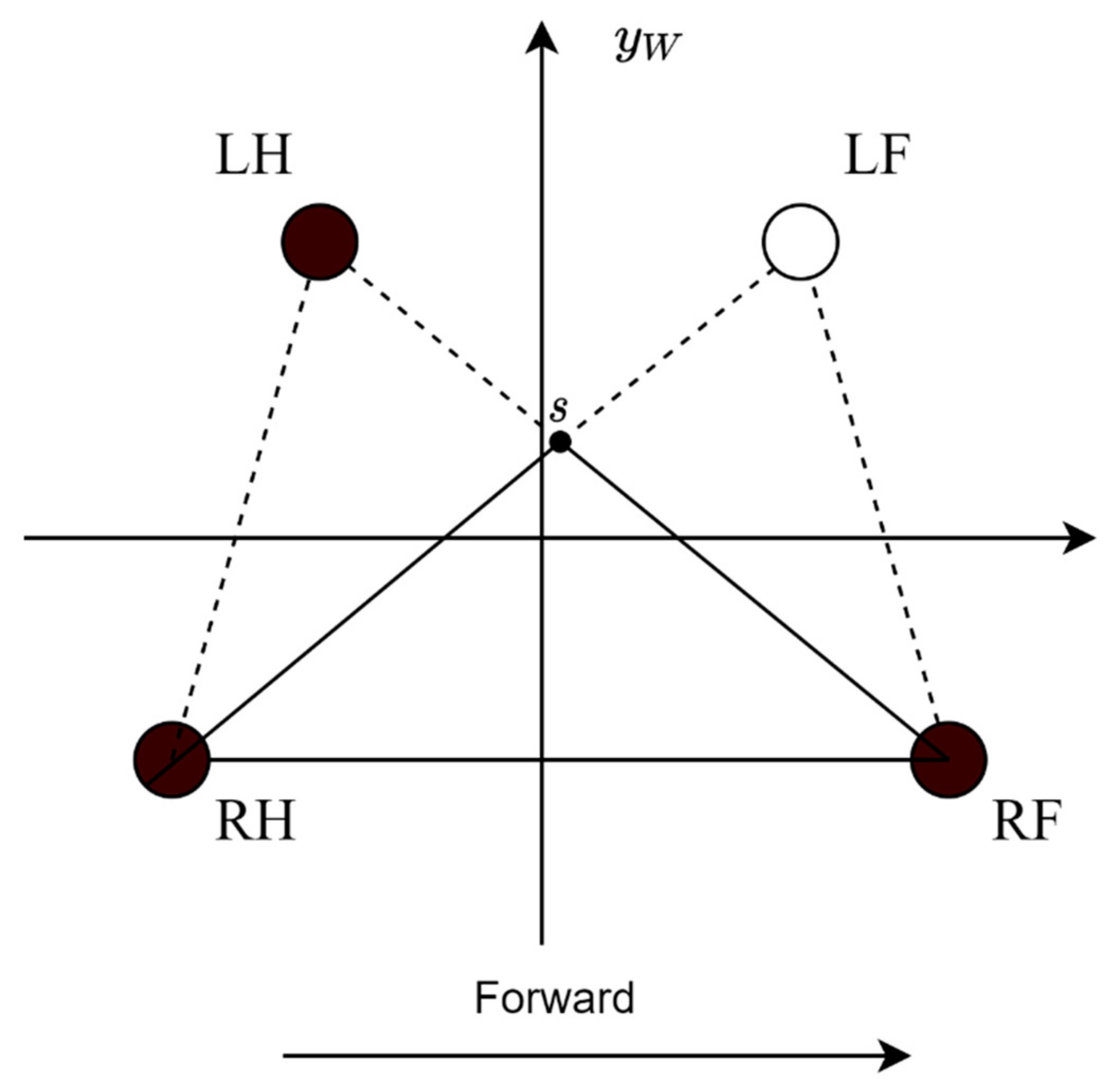
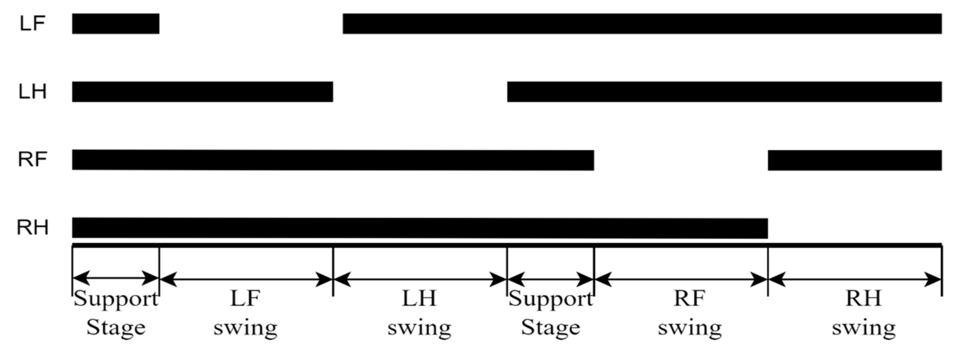
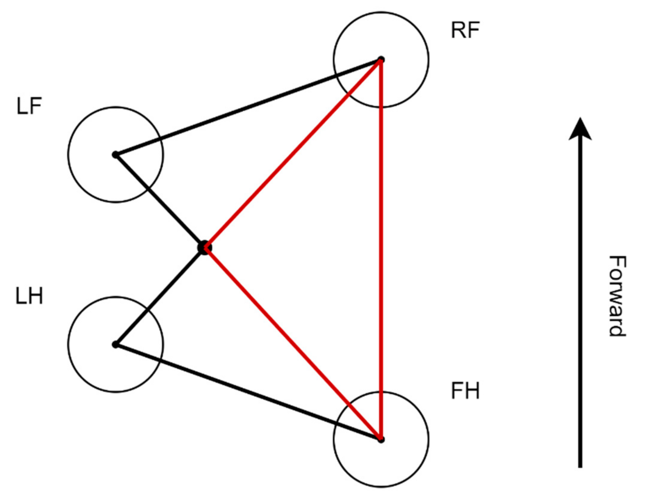
Assume that the coordinates of the center of gravity of the robot are $\left(x_C,y_C,z_C\right)$. According to Equation (11), the desired coordinate position of ZMP can be obtained as $\left(x_I,y_I\right)$. According to the “cart-table” model proposed in [13], the equation between the barycentric coordinates and the ZMP coordinates can be obtained as follows:

$$\left\{\begin{array}{c}\ddot{x_C}=\frac{g}{z_C}\left(x_C-x_I\right)\\ \ddot{y_C}=\frac{g}{z_C}\left(y_C-y_I\right)\end{array}\right.$$

(12)

where g is gravity acceleration and $\ddot{x_C}$ and $\ddot{y_C}$ are the acceleration of the robot’s center of mass along the X-axis and Y-axis, respectively.

The differential equations are solved as follows:

$$x_C=\frac{g}{z_C}+C_1{e}^{\sqrt{\frac{g}{z_C}}t}+C_2{e}^{-\sqrt{\frac{g}{z_C}}t}$$

(13)

$$y_C=\frac{g}{z_C}+C_3{e}^{\sqrt{\frac{g}{z_C}}t}+C_4{e}^{-\sqrt{\frac{g}{z_C}}t}$$

(14)

where $C_1, C_2,C_3, \mathrm{a}\mathrm{n}\mathrm{d} C_4$ are constant coefficients. It is known that the position of the center of gravity in the quadruped support stage is the initial position, and to ensure that the trajectory of the center of gravity is continuous and the speed of the center of gravity has no sudden change, in the foot swing stage, the robot’s torso remains stationary, and its speed and acceleration are both zero.

Therefore, when we know the coordinates of the ZMP and the coordinates of the center of gravity at the initial moment, we can obtain the position of the center of gravity at the next moment. Then, according to the matrix transformation, the position of the coordinates of the desired landing point can be obtained.

3.3. Gait Planner

For quadruped robots, there are six non-singular static gaits [2]. This paper designs a crawl gait. Crawl gait has good stability when walking at low speed and has high adaptability to challenging terrain. The crawling gait is supported by at least three legs at any time. The leg swing sequence of the robot designed in this paper is: LF → LH → RF → RH. Considering that when the swinging leg of the robot switches from the left (right) side to the right (left) side, the stable support triangle of the robot switches from right to left. In this paper, the quadruped support phase is added to the swing cycle of the robot to ensure a smooth transition. We divided one motion cycle of a quadruped robot into six stages: Support Stage → LF swing → LH swing → Support Stage → RF swing → RH swing. The sequence diagram of the quadruped robot crawling gait is shown in Figure 6.

Take the left swing leg exercise as an example, in which the right leg is always in a supported state. When the LF leg swings, the LH leg and the right leg form a supporting triangle. Additionally, when the LH leg swings, the LF leg and the right leg form a supporting triangle. The two supporting triangles have overlapping parts, which constitute the right stable support domain (the red triangle in Figure 7). The robot can maintain a stable motion state when the ZMP of the robot is in this region.

3.4. Foot Trajectory Planner

Foot trajectory planning is an important part of quadruped robot motion control. Refs. [14,15,16] used the CPG, interpolation curve, and sinusoidal parameterized gait control strategy, respectively, and successfully applied them to the quadruped robot. In this paper, the Bezier curve is used to plan a semi-elliptical trajectory to realize the parametric control of the foot trajectory of the quadruped robot. The semi-elliptical trajectory is shown in Figure 8.

The Bezier curves, which are related to Bernstein polynomials, are named after the French engineer Pierre Bézier, who used it in the 1960s for designing curves for the bodywork of Renault cars. We chose to parameterize the end-foot trajectory of each foot by a Bezier curve. Bezier Curves have attractive properties over other alternatives, such as quintic splines, because they do not have self-intersecting curves, and are guaranteed to lie within the convex hull of the control points. This ensures that the trajectories are always in the workspace of the end-effector [17,18].

The shape of the Bezier curve is determined by the control points. A Bezier equation of degree n in the plane requires n + 1 control points that denoted by $P_i\left(i=0,1,\cdots n\right)$. The curve starts at point $P_0$ and goes to point $P_n$. Generally, it does not pass through the middle point, and the middle point only plays a guiding role. The higher-order Bezier curve equation is:

$$B\left(t\right)={\displaystyle \sum }_{i=0}^n\left(\begin{array}{c}n\\ i\end{array}\right)P_i{\left(1-t\right)}^{n-i}{t}^i=\left(\begin{array}{c}n\\ 0\end{array}\right)P_0{\left(1-t\right)}^n{t}^0+ \dots +\left(\begin{array}{c}n\\ n\end{array}\right)P_n{\left(1-t\right)}^0{t}^n$$

(15)

where $t\in [0, 1]$ and $B\left(t\right)$ are the Bezier curve polynomials.

The crawling gait in this paper has a total of six stages and can be divided into two states: the stance state and the swing state. When the robot leg is swinging, the trajectory generator takes the robot’s current footfall point and expected footfall point as input, and uses the Bezier curve to plan the swinging leg to generate a semi-elliptical trajectory, as shown in the following formula:

$$S_{tg}={\displaystyle \sum }_{k=0}^n\left(\begin{array}{c}n\\ k\end{array}\right)t^k{\left(1-t\right)}^{n-k}{p}_k\left(x,y\right)$$

(16)

where $S_{tg}$ is the trajectory generator equation. Our Bezier curves use 9 control points (see

Table 1. Bezier curve control points.

Pi	X	Y
0	xp	yp
1	−0.05 (xd − xp)	yp
2	−3 (xd − xp)	0.9 (yp − yd)
3	xp	1.1 (yp + yd)
4	0.5 (xd − xp)	1.2 (yp + yd)
5	(xd − xp)	1.1 (yp + yd)
6	1.1 (xd − xp)	0.09 (yp + yd)
7	1.05 (xd − xp)	yd
8	xd	yd

). $p_k\left(x,y\right)$ is the control point, which is controlled by the robot’s current landing point, $\left(x_p,y_p\right)$, and the desired landing point, $\left(x_d,y_d\right)$.

Given different landing points, different foot trajectories can be generated. After the calculation of inverse kinematics, the motor commands required by the 12 motors of the robot are obtained, to control the walking of the quadruped robot on the slope.

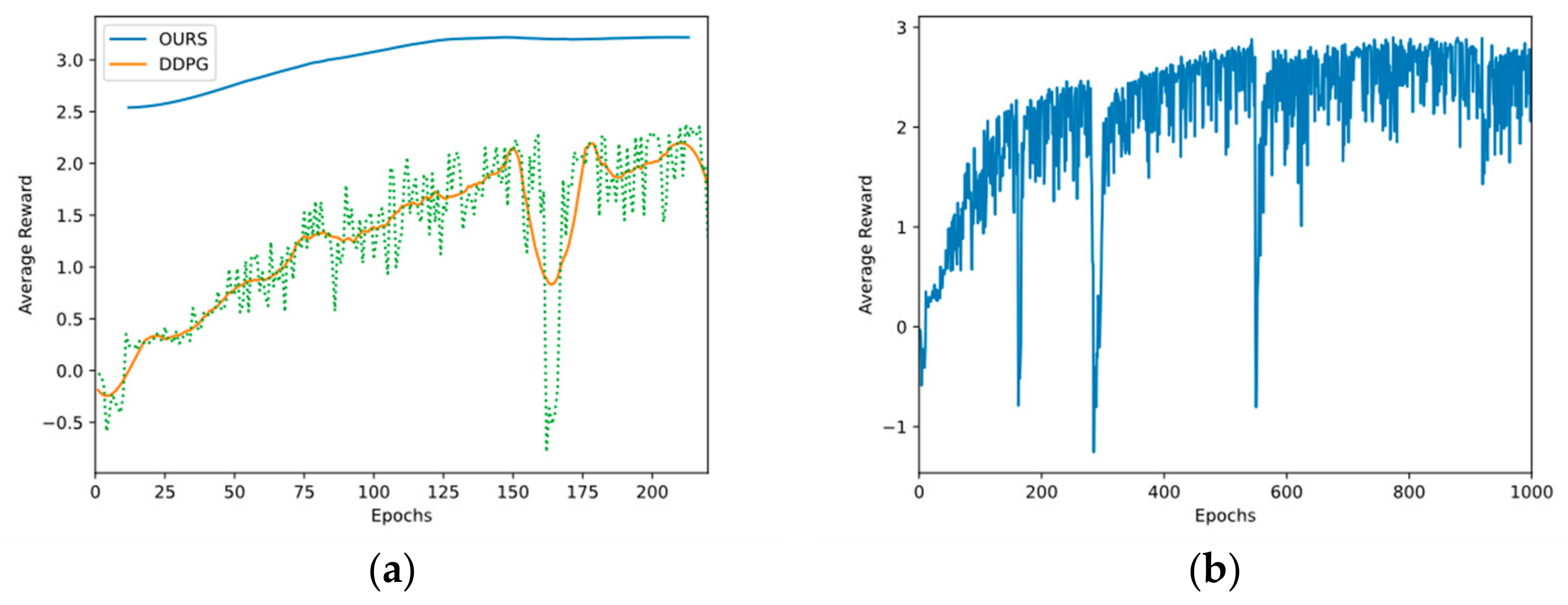
3.5. Training Algorithm

The stable walking problem of the quadruped robot on slopes in this paper can be regarded as a partially observable Markov decision problem (MDP). MDP is described for each time step t with a tuple, {s, a, p, r, y}, where s is the current robot state, a is the action applied, p is the transition probability function from the current state, $s_t$, to the next state $s_{t+1}$, r is a reward value obtained due to the transition, and $y\subset \left(0,1\right)$ is a discount factor for the long-term reward [19].

The goal of reinforcement learning is to find an optimal strategy to maximize the cumulative reward value, as shown in Equation (17). In this paper, we train a linear policy $a_t=\pi \left(\theta ,o_t\right)$ to enable the robot to receive information in the environment, so that it can output the optimal action to maximize the cumulative reward.

$${\theta }^{\ast }=argma{x}_{\theta }\mathbb{E}\left[{\displaystyle \sum }_{t=0}^{T-1}{\gamma }^t{r}_t\right]$$

(17)

where $\mathbb{E}$ is the expect reward, and T is the total timesteps.

In this paper, the augmented random search (ARS) [20] algorithm is chosen to find a linear policy. ARS is a model-free reinforcement learning algorithm, which adopts a gradient-free policy gradient method, which greatly reduces the complexity of the algorithm and can achieve the training effect of other model-free reinforcement learning algorithms.

The ARS algorithm abandons the differential-based policy gradient method and uses the finite difference method to approximate the gradient from the sampling of multiple directional derivatives, so there is no differentiation process. We used Version V-1t of ARS from [20]. For a given strategy, the policy is perturbed both along the positive and negative directions, ${\theta }_t+\upsilon {\delta }_{\left(k\right)}$, ${\theta }_t-\upsilon {\delta }_{\left(k\right)}$.

$${\theta }_{t+1}={\theta }_t+\frac{\alpha }{b\ast {\sigma }_R}{\displaystyle \sum }_{k=1}^b\left[r\left({\theta }_t+\upsilon {\delta }_{\left(k\right)}\right)-r\left({\theta }_t-\upsilon {\delta }_{\left(k\right)}\right)\right]{\delta }_{\left(k\right)}$$

(18)

where α is the step size, and ${\sigma }_R$ is the standard deviation, and $\upsilon <1$ is a constant. ${\delta }_{\left(k\right)}$ is a sample taken from a standard normal distribution. b is a constant which is the best b directions corresponding to the maximum returns.

The reward function designed in this paper is used to guide the robot to adapt to the terrain slope and move in the forward direction. We obtain the following:

$$r=5x-\left(\left|{∆}_P^r-{∆}_P\right|+\left|{∆}_R^r-{∆}_R\right|\right)-2{∆}_Y^r$$

(19)

where r is the cumulative reward, and x is the horizontal distance that the robot’s center of gravity moves in the direction of motion. ${∆}_P^r,{∆}_R^r, \mathrm{a}\mathrm{n}\mathrm{d} {∆}_Y^r$ are the actual pitch angle, roll angle, and yaw angle of the quadruped robot during the movement process, respectively, which we can obtain this data from the IMU; ${∆}_P$, ${∆}_R$ are the desired pitch and roll, respectively. The units of ${∆}_P^r,{∆}_R^r,{∆}_Y^r,{∆}_P, \mathrm{a}\mathrm{n}\mathrm{d} {∆}_R$ are the angles.

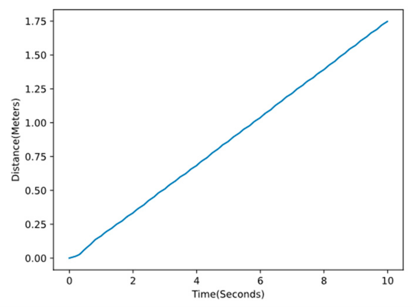
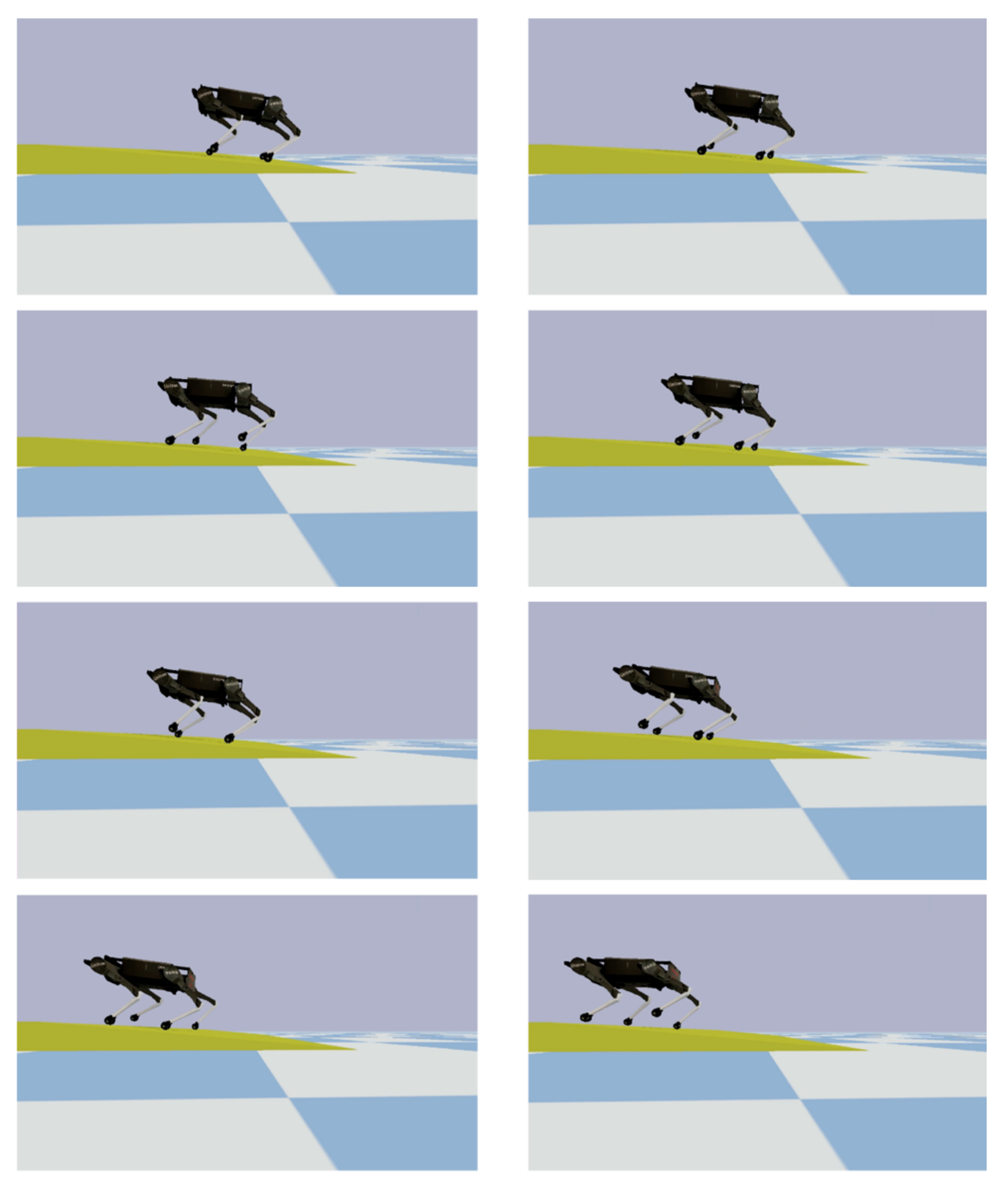
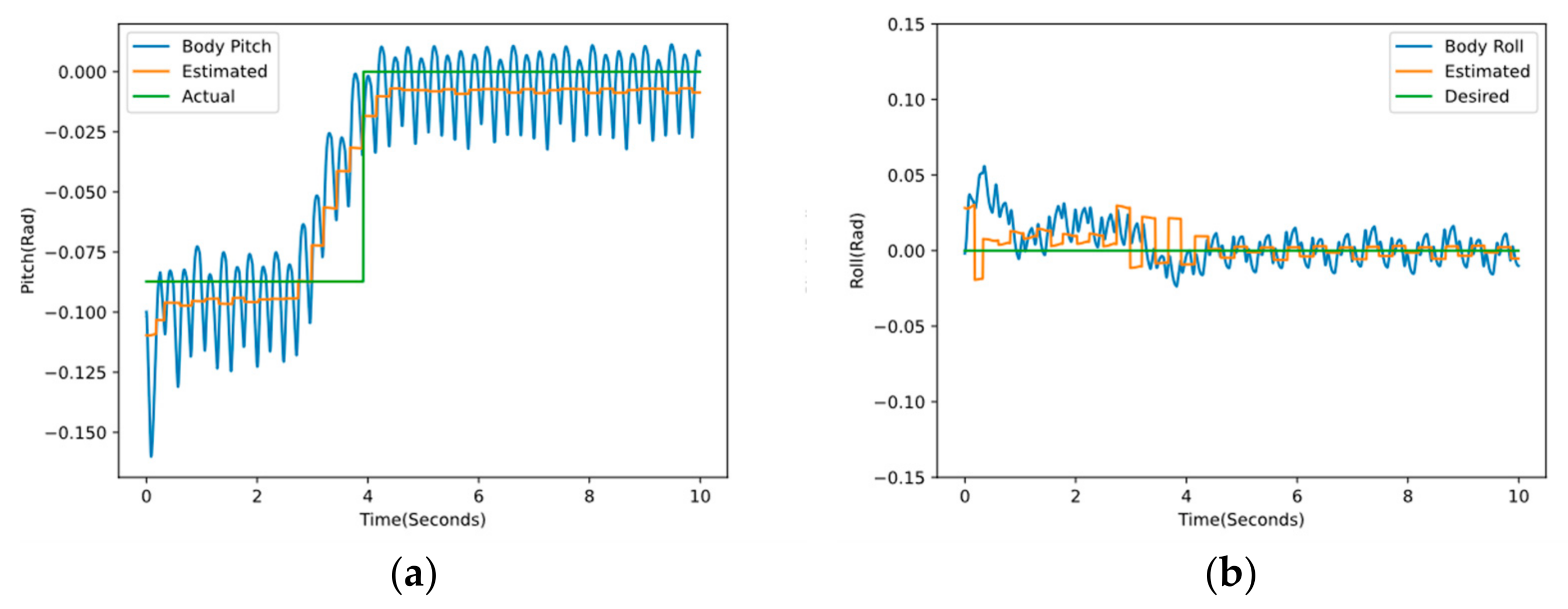
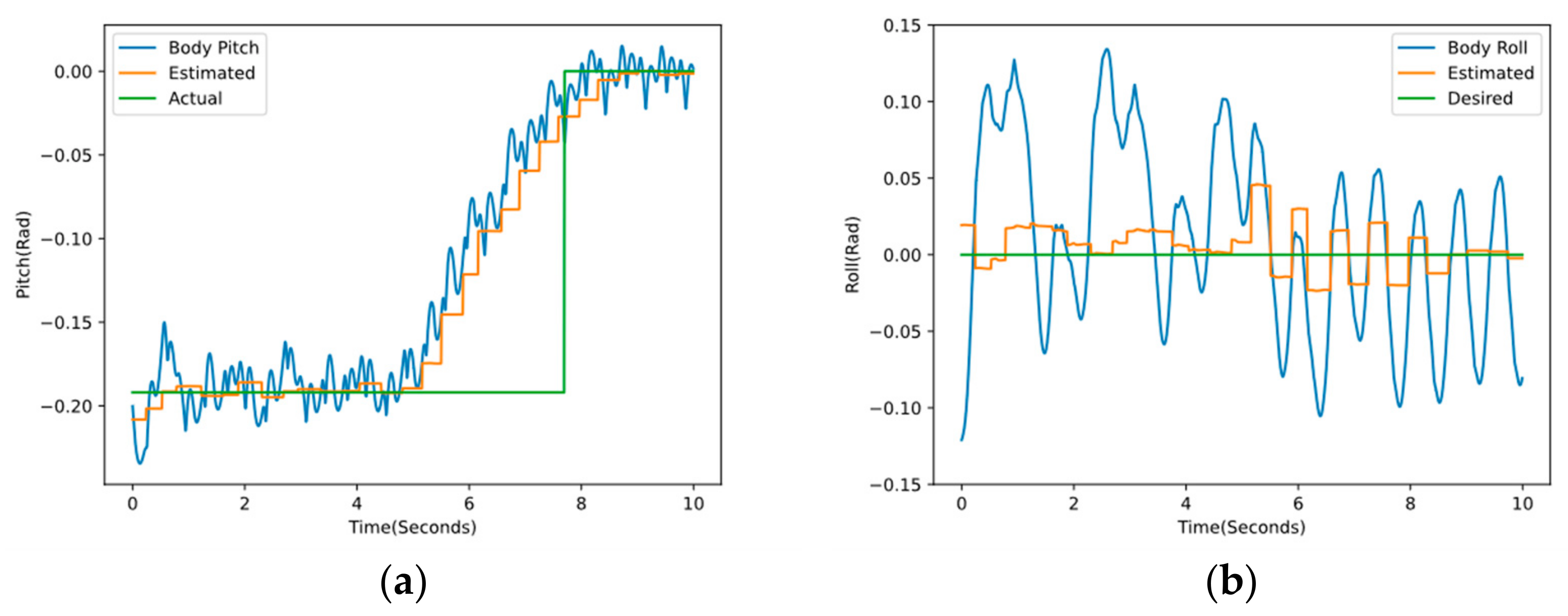
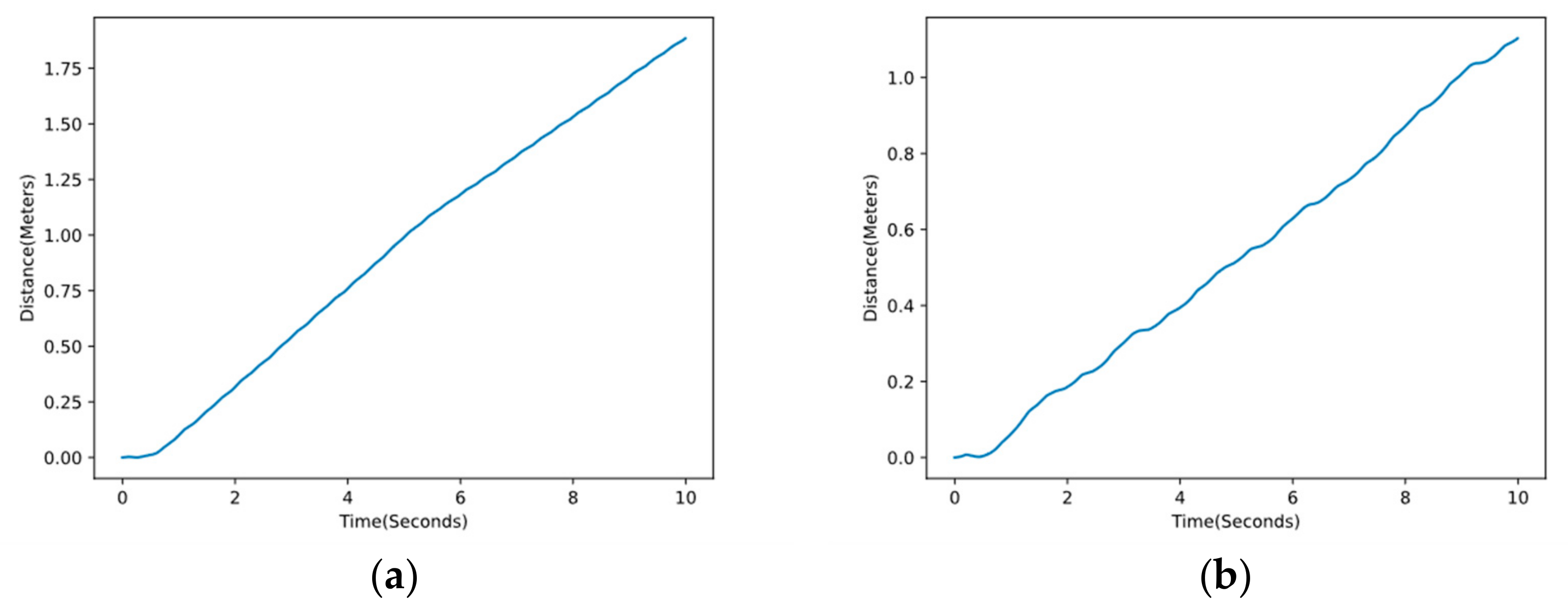
4. Results and Discussion

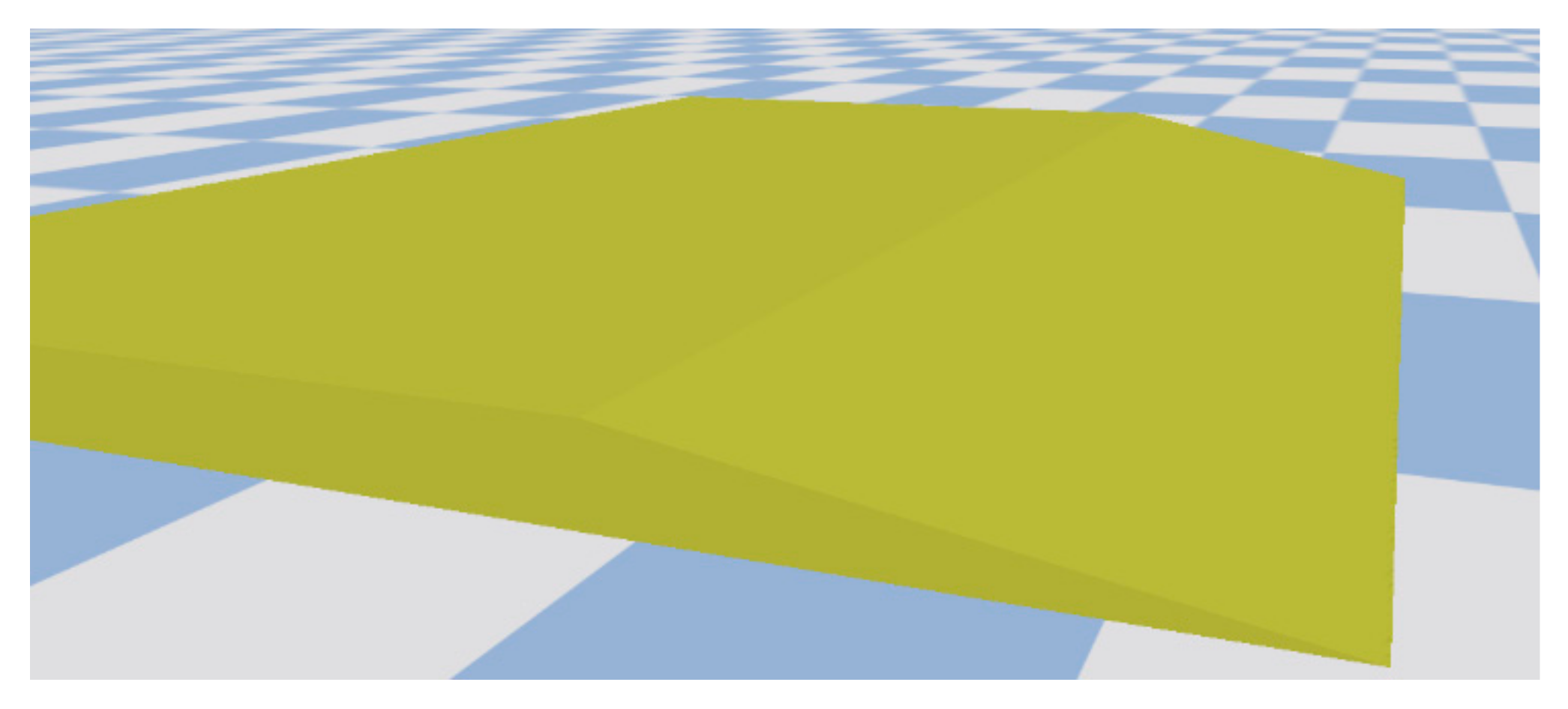
4.1. Simulation Environment

As shown in Figure 9, the simulation model of the robot is shown. Each leg of the robot has three degrees of freedom, namely the pitching hip joint, the pitching knee joint, and the rolling hip joint. The robot joints are controlled by high-performance motors, and the total instantaneous maximum power that can be reached is 18 kw.

Laikago’s torso is 0.55 m long and 0.35 m wide. When standing naturally, the height is 0.6 m, and the weight of the whole machine is about 24 kg. An inertial measurement unit (IMU) is installed on the trunk of the machine to detect the attitude of the robot and the speed and acceleration information of the trunk. A force sensor is installed at the foot-end of the robot to sense information [21].

Figure 10 shows the slope built on Pybullet [22] platform. In this simulation experiment, the algorithm is tested on 0° slope (plane), 5° slope, and 11° slope, respectively.

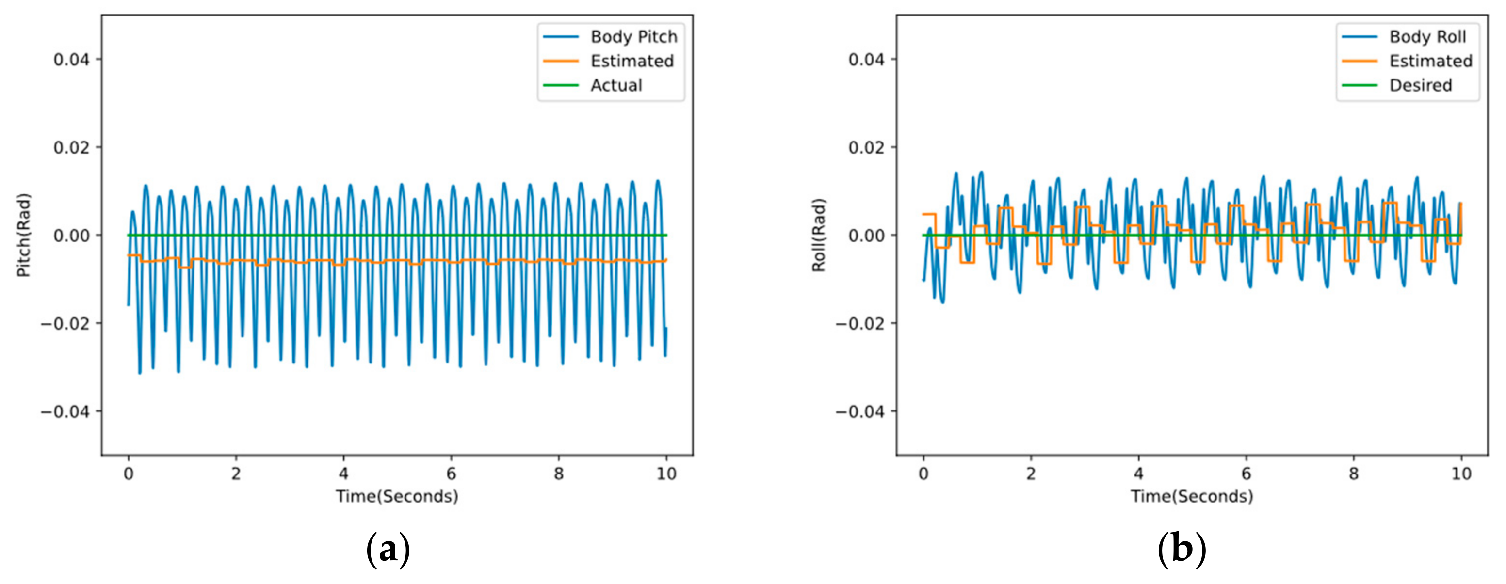
4.2. Results and Discussion

To verify that parameterized foot trajectories can speed up robot learning, we compared the algorithm proposed in this paper with the reinforcement learning algorithm deep deterministic policy gradient (DDPG). DDPG is a class of model-free reinforcement learning algorithms that perform well in control tasks with continuous action spaces. Our algorithm uses the ARS algorithm to optimize foot trajectories parameterized by Bezier curves, while DDPG is trained from scratch.

We trained the robot for 400 epochs, and the maximum timestep of each epoch was 2000 steps. Figure 11 shows the average reward value of each round of the robot in the simulation environment. According to Figure 11a, our algorithm can converge in about 150 epochs, while the DDPG algorithm is still in the rising stage, and the policy is very unstable. Next, we trained the DDPG algorithm for 1000 epochs, as shown in Figure 11b, and found that the algorithm stabilized around 800 epochs.

From the training results, it can be seen that the reinforcement learning algorithm trained from scratch needs to explore the environment at the beginning of training, and can only train the robot after accumulating data. However, our use of Bezier curves to parameterize the robot foot trajectory is to integrate the prior knowledge into the foot trajectory generator, which reduces the complexity of the policy learning problem and greatly reduces the training time.

Figure 12 shows the changes of body pitch angle and roll angle in the walking simulation experiment of the robot facing a 0° slope. The green line is the real slope of the terrain, and the orange line is the estimated value of the slope by the terrain estimation algorithm. Additionally, the blue line is the change of the pitch angle and roll angle of the robot obtained from the robot IMU.

It can be seen from Figure 12 that the terrain estimation algorithm proposed in this paper can effectively estimate the slope, and the pitch angle and the roll angle of the robot can fluctuate within a certain range through algorithm learning, to ensure the stability of the robot in the process of moving.

Table 2. The data of the terrain estimation.

	Actual Value	Average Value	Standard Error	Maximum Deviation
E-Pitch	0	−0.005894	0.000013	−0.007399
E-Roll	0	0.000543	0.000108	0.007371

shows the data analysis of the terrain estimation. The standard error between the estimated pitch angle and the true value is 0.000013, and the maximum deviation is 0.007399; additionally, the standard error between the estimated roll angle and the true value is 0.000108, and the maximum deviation is 0.007371. The effectiveness of the terrain estimation algorithm is fully illustrated.

Table 3. The data from the IMU of robot.

	Average Value	Standard Deviation	Maximum
R-Pitch	−0.003629	0.012690	−0.031460
R-Roll	0.001382	0.007026	−0.015340

shows the data analysis of real pitch angle and roll angle during robot movement. The average swing angle of the robot is less than −0.003629 rad (<1°), and the max swing angle is less than 0.007026 rad (<2°). The robot can walk stably, which shows the effectiveness of the trajectory generator.

Figure 13 shows the horizontal distance that the robot’s center of mass travels along the robot’s motion direction in the 10 s time in the walking simulation experiment of the robot facing a 0° slope. From this, it can be seen that the motion trajectory of the robot is continuous and moves forward.

Figure 14 shows a screenshot of the robot moving on the slope. According to the gait planning algorithm framework of the quadruped robot proposed in this paper, the robot can effectively predict the slope and adjust the robot’s attitude to realize stable walking on the slope.

Figure 15 and Figure 16 show the changes of body pitch angle and roll angle during the walking simulation experiment of the robot facing a 5° and 11° slope, respectively. The green line is the true slope of the terrain, the orange line is the estimated value of the slope by the terrain slope estimation algorithm, and the blue line is the change of the pitch angle and roll angle of the robot obtained from the IMU.

According to Figure 15a and Figure 16a, the curve is divided into three sections. The first section on the left shows that the robot is standing on the slope; the second segment indicates that the robot adaptively adjusts the attitude to follow the change of the estimated value according to the terrain slope estimation algorithm and ARS algorithm; in the third section, after a period of motion, the robot successfully walked to the platform at the top of the slope, which fully shows the feasibility and effectiveness of this research algorithm.

Figure 17 shows the horizontal distance traveled by the robot’s center of mass along the robot’s motion direction in the 10 s time in the simulation experiment of the robot facing the 5° slope and the 11° slope. Although, the increase in slope has a certain impact on the movement speed of the robot. However, the trajectory of the robot is continuous and moving forward.

5. Conclusions

In this paper, an adaptive motion skill learning of the quadruped robot on slopes was proposed to realize the stable walking of a quadruped robot on 5° and 11° slopes. First of all, a terrain slope estimation algorithm was proposed, in which the slope was estimated according to the robot foothold, to obtain the desired body attitude angle of the robot. Then, the augmented random search (ARS) algorithm was used for training a motion strategy of the quadruped robot so that the quadruped robot can adaptively adjust its attitude to follow the desired body attitude angle. In addition, the Bezier curve was used to parameterize the robot trajectory, which greatly sped up the learning speed. The feasibility and effectiveness of the algorithm framework were verified in the simulation environment. The robot can adaptively adjust its attitude to realize its motion on the slope and maintain good stability. The sim-to-real transition is very interesting and challenging work—to further validate our algorithm, we plan to deploy physical experiments in future work.

References

1. Yang, J.; Sun, H.; Wang, C.; Chen, X. An Overview of Quadruped Robots. Navig. Position. Timing 2019, 6, 61–73. [Google Scholar]
2. Mcghee, R.B.; Frank, A. On the stability properties of quadruped creeping gaits. Math. Biosci. 1968, 3, 331–351. [Google Scholar] [CrossRef]
3. Hwang, H.; Youm, Y. Steady crawl gait generation algorithm for quadruped robots. Adv. Robot. 2008, 23, 1539–1558. [Google Scholar] [CrossRef]
4. Kalakrishnan, M.; Jonas, B.; Peter, P.; Michael, N.M.; Stefan, S. Learning, planning, and control for quadruped locomotion over challenging terrain. Int. J. Robot. Res. 2011, 30, 236–258. [Google Scholar] [CrossRef]
5. Ijspeert, A.J. Central pattern generators for locomotion control in animals and robots: A review. Neural Netw. 2008, 21, 642–653. [Google Scholar] [CrossRef] [PubMed]
6. Montesdeoca, J.C.; Santos, M.C.P.; Monllor, M.; Herrera, D. Trajectory tracking controller for differential-drive mobile robots. In Proceedings of the 2017 XVII Workshop on Information Processing and Control (RPIC), Mar del Plata, Argentina, 20–22 September 2017; pp. 1–4. [Google Scholar]
7. Kimura, H.; Yasuhiro, F.; Cohen, A.H. Adaptive Dynamic Walking of a Quadruped Robot on Natural Ground Based on Biological Concepts. Int. J. Robot. Res. 2007, 26, 475–490. [Google Scholar] [CrossRef]
8. Gehring, C.; Bellicoso, C.D.; Coros, S.; Bloesch, M.; Fankhauser, P.; Hutter, M.; Siegwart, R. Dynamic trotting on slopes for quadrupedal robots. In Proceedings of the 2015 IEEE/RSJ International Conference on Intelligent Robots and Systems (IROS), Hamburg, Germany, 28 September–2 October 2015; pp. 5129–5135. [Google Scholar]
9. Kohl, N.; Peter, S. Policy gradient reinforcement learning for fast quadrupedal locomotion. In Proceedings of the IEEE International Conference on Robotics and Automation, New Orleans, LA, USA, 26 April–1 May 2004; Volume 3, pp. 2619–2624. [Google Scholar]
10. Iscen, A.; Caluwaerts, K.; Tan, J.; Zhang, T.; Coumans, E.; Sindhwani, V.; Vanhoucke, V. Policies Modulating Trajectory Generators. arXiv 2019, arXiv:1910.02812. [Google Scholar]
11. Lee, J.; Jemin, H.; Lorenz, W.; Vladlen, K.; Marco, H. Learning quadrupedal locomotion over challenging terrain. Sci. Robot. 2020, 5, eabc5986. [Google Scholar] [CrossRef] [PubMed]
12. Vukobratovic, M.; Borovac, B. Zero-moment point: Thirty five years of its life. Int. J. Hum. Robot. 2004, 1, 157–173. [Google Scholar] [CrossRef]
13. Kajita, S.; Fumio, K.; Kenji, K.; Kiyoshi, F.; Kensuke, H.; Kazuhito, Y.; Hirohisa, H. Biped walking pattern generation by using preview control of zero-moment point. In Proceedings of the 2003 IEEE International Conference on Robotics and Automation (Cat. No.03CH37422), Taipei, Taiwan, 14–19 September 2003; Volume 2, pp. 1620–1626. [Google Scholar]
14. Wei, Y.; Zhou, C.; Guo, J.; Xu, P. CPG-based Stable Walking Control of the Quadruped Robot on the Slope. Control. Eng. China 2021, 28. [Google Scholar] [CrossRef]
15. Tirumala, S.; Sagi, A.; Paigwar, K.; Joglekar, A.; Bhatnagar, S.; Ghosal, A.; Kolathaya, S. Gait Library Synthesis for Quadruped Robots via Augmented Random Search. arXiv 2019, arXiv:1912.12907. [Google Scholar]
16. Paigwar, K.; Krishna, L.; Tirumala, S.; Khetan, N.; Sagi, A.; Joglekar, A.; Kolathaya, S. Robust Quadrupedal Locomotion on Sloped Terrains: A Linear Policy Approach. arXiv 2020, arXiv:2010.16342. [Google Scholar]
17. Chen, C.; He, Y.-Q.; Bu, C.-G.; Han, J.-D. Feasible trajectory generation for autonomous vehicles based on quartic B’ezier curve. Acta Autom. Sin. 2015, 41, 486–496. [Google Scholar]
18. Tirumala, S.; Gubbi, S.; Paigwar, K.; Sagi, A.; Joglekar, A.; Bhatnagar, S.; Kolathaya, S. Learning stable manoeuvres in quadruped robots from expert demonstrations. In Proceedings of the 2020 29th IEEE International Conference on Robot and Human Interactive Communication (RO-MAN), Naples, Italy, 31 August–4 September 2020; pp. 1107–1112. [Google Scholar]
19. Sewak, M. Deep Reinforcement Learning: Frontiers of Artificial Intelligence; Springer: Berlin/Heidelberg, Germany, 2019. [Google Scholar] [CrossRef]
20. Mania, H.; Aurelia, G.; Benjamin, R. Simple random search of static linear policies is competitive for reinforcement learning. Adv. Neural Inf. Processing Syst. 2018, 31. Available online: https://proceedings.neurips.cc/paper/2018/hash/7634ea65a4e6d9041cfd3f7de18e334a-Abstract.html (accessed on 5 March 2022).
21. Guizzo, E. This Robotics Startup Wants To Be the Boston Dynamics of China. Available online: https://spectrum.ieee.org/automaton/robotics/robotics-hardware/this-robotics-startup-wants-to-be-the-boston-dynamics-of-china (accessed on 5 March 2022).
22. Coumans, E.; Bai, Y. Pybullet, a Python Module for Physics Simulation for Games, Robotics and Machine Learning. Available online: http://pybullet.org/wordpress/ (accessed on 5 March 2022).
Figure 1. Algorithm frame.
Electronics 11 00842 g001
Figure 2. Robot model.
Electronics 11 00842 g002
Figure 3. Figure showing the foot position vectors used for the slope estimator.
Electronics 11 00842 g003
Figure 4. Figure showing the projection point of the robot foot on the ground.
Electronics 11 00842 g004
Figure 5. Figure showing the coordinates of projection in the world coordinate system.
Electronics 11 00842 g005
Figure 6. Sequence diagram of crawling gait.
Electronics 11 00842 g006
Figure 7. Support domain.
Electronics 11 00842 g007
Figure 8. Semi-elliptical trajectory.
Electronics 11 00842 g008
Figure 9. Laikago’s model.
Electronics 11 00842 g009
Figure 10. The simulation model of 5° slope.
Electronics 11 00842 g010
Figure 11. Average reward during robot training. (a) Ours vs. DDPG. (b) DDPG.
Electronics 11 00842 g011
Figure 12. Changes in the attitude angle of the robot. (a) Changes in the pitch angle of the robot. (b) Changes in the roll angle of the robot.
Electronics 11 00842 g012
Figure 13. Picture showing the distance the center of gravity has moved.
Electronics 11 00842 g013
Figure 14. Robot moving on a slope.
Electronics 11 00842 g014
Figure 15. Changes in the attitude angle of the robot on the 5° slope. (a) Changes in the pitch angle of the robot on the 5° slope. (b) Changes in the roll angle of the robot on the 5° slope.
Electronics 11 00842 g015
Figure 16. Changes in the attitude angle of the robot on the 11° slope. (a) Changes in the pitch angle of the robot on the 11° slope. (b) Changes in the roll angle of the robot on the 11° slope.
Electronics 11 00842 g016
Figure 17. Picture showing the distance the center of gravity has moved. (a) The distance the center of gravity has moved on the 5° slope. (b) The distance the center of gravity has moved on the 11° slope.
Electronics 11 00842 g017