Optimization of Intrusion Detection Systems Determined by Ameliorated HNADAM-SGD Algorithm

Abstract

Information security is of pivotal concern for consistently streaming information over the widespread internetwork. The bottleneck flow of incoming and outgoing data traffic introduces the issues of malicious activities taken place by intruders, hackers and attackers in the form of authenticity obstruction, gridlocking data traffic, vandalizing data and crashing the established network. The issue of emerging suspicious activities is managed by the domain of Intrusion Detection Systems (IDS). The IDS consistently monitors the network for the identification of suspicious activities, and generates alarm and indication in the presence of malicious threats and worms. The performance of IDS is improved by using different machine learning algorithms. In this paper, the Nesterov-Accelerated Adaptive Moment Estimation–Stochastic Gradient Descent (HNADAM-SDG) algorithm is proposed to determine the performance of Intrusion Detection Systems IDS. The algorithm is used to optimize IDS systems by hybridization and tuning of hyperparameters. The performance of algorithm is compared with other classification algorithms such as logistic regression, ridge classifier and ensemble algorithms where the experimental analysis and computations show the improved accuracy with 99.8%, sensitivity with 99.7%, and specificity with 99.5%.

1. Introduction

The extensive practice of technology over a widespread network introduces the importance of information security. The illegitimate activities of intruders are kept under consistent monitoring, provided by different security software such as firewalls, anti-malware systems, anomaly detection systems, endpoint systems and IDS. The availability of on demand resources allows users to store the voluminous amount of data and information over the service provider’s platform, where the platforms are open sourced software, open clouds and integrated development environments. The extent of exposure to virtual resources give arise to the evolving problem of virtual security threats. Ref. [1] found that security threats can arise within the network or outside the network by multiple intruders in the form of cyber-attacks, malware and worms. IDS are detection systems that track malicious activities by monitoring incoming and outgoing network traffic, the alarm or alerts are generated based on the identification of unusual activities within the network. The alarm is generated if the intruder attempts to hamper the virtual security by gaining unauthorized access to the private network, wide area network, personal network, personal computer and large scale computer hubs by passing information to the administration of the security breach. The IDS system aims to catch the suspicious activity of intruders or hackers before they forge the information by crashing the network system. The IDS are defined as network based IDS, host based IDS, signature based IDS and anomaly based IDS. The one of the most popularly used IDS is SNORT, which usually works on a Unix or Linux based operating system with a lightweight network based IDS [2]. The IDS system installed over any network is used for the detection of malicious activities and to keep track of different types of cyber-attacks imposed over the network. The recorded attack patterns help to identify future attack occurrences in any organization, to change and adopt the enhanced security systems. It is able to track bugs or network configurations. The IDS sensory devices are the other methodology to make the system more secure and sustainable, by using an alarm filtering technique to differentiate between malicious and normal activity patterns.

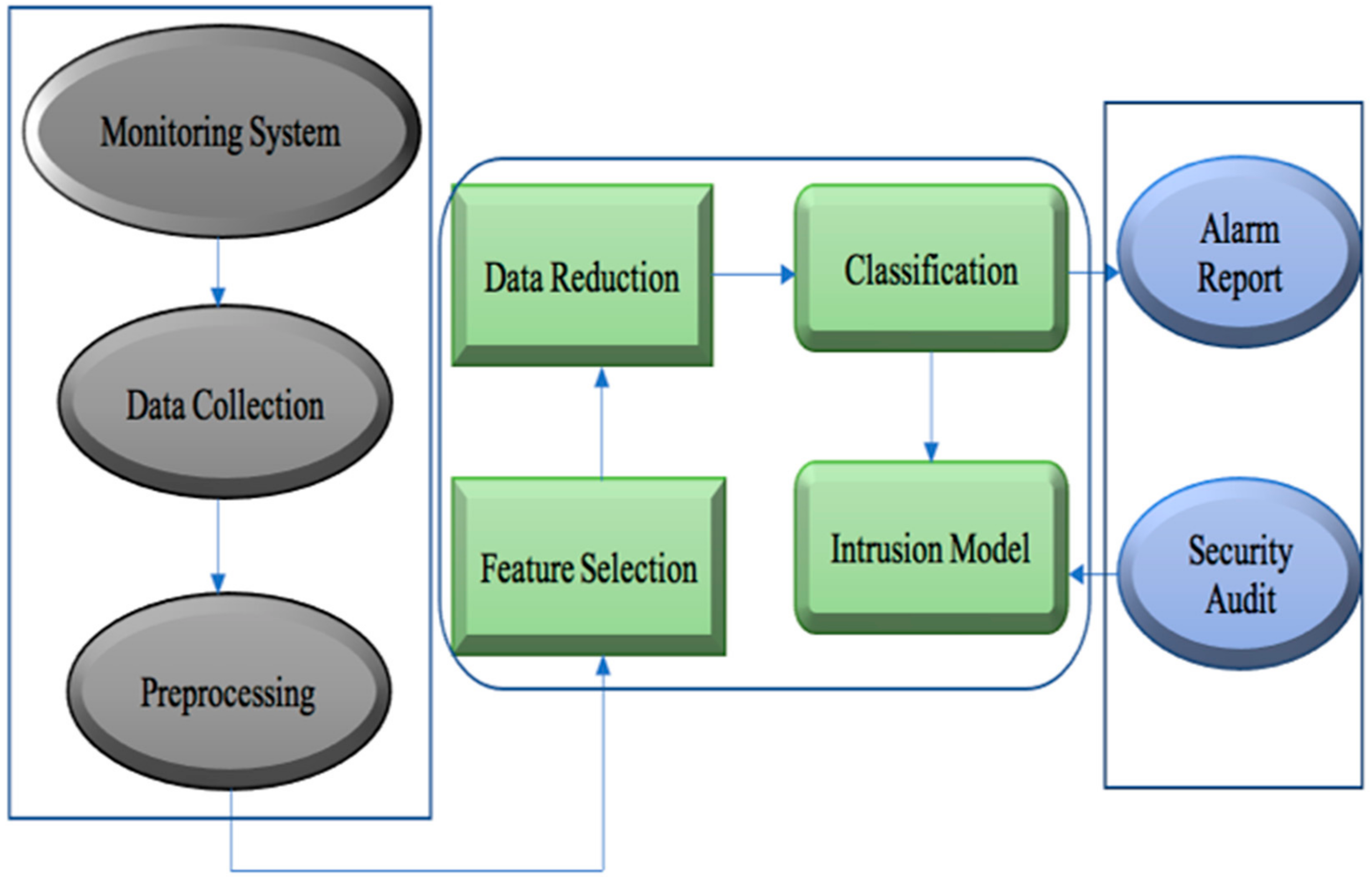
The Figure 1 shows the schematic representation of IDS [3]. This is the illustration for designing an IDS model where hypertuning and optimization is the technique. The methodology to design a machine learning algorithm with a good classification and prediction result involves data collection, data preprocessing, feature selection, data reduction and classification [4]. The IDS works as a monitoring system that constantly tracks incoming and outgoing network traffic. The network attack and malicious activity is captured in the form of data which are then used for understanding attack patterns and for changing the security model on the basis of updated attack patterns.

Gap Analysis

The hyperparameter optimization algorithms’ performance depends on various factors such as total hidden layers, total per-layer units, dropout amount, regularizer learning rate and weight decay. The non-optimal setting of hyperparameters will drastically affect the algorithm performance, that varies from an extremely low learning rate to a very large learning rate. The cogency of the paper is defined as finding the hyperparameter optimization methodology for a UNSW-NB15 dataset to gain higher accuracy by minimizing the generalization error. The proposed HNADAM-SDG algorithm trains the network with only a subset of hyperparameter configurations where the subset of configuration is randomly opted. The hyperparameters are defined before the model training to provide the flexibility to fit the model on the basis of dataset. The compulsions of the gradient descent algorithm are accelerated by the optimization of the hyperparameters. The performance analysis and experimental analysis of the algorithm is compared with other classification algorithms by adapting the hyperparameter optimization and feature selection techniques. The research questions for the paper are:

• RQ1—To find the combination of hyperparameters to maximize the performance of model by diminishing generalization error and computational cost.
• RQ2—To find a hyperparameter response space which depends on methodology, hyperparameters, dataset and metrics.
• RQ3—To deploy a methodology by the sampling of candidate parameters using a cross-validation scheme.

The paper is presented by combining multiple sections, as Section 2 represents related work. The detailed description of the dataset has been explained in Section 3, and the detailed explanation of the methodology used in the proposed algorithm has been explained in Section 4. In Section 5, the proposed algorithm has been explained in detail, in Section 6, the results observed from the proposed algorithm and the discussion of the result has been done, and in Section 7, the conclusion of the proposed work has been explained.

2. Related Work

In the recent research trends, it has been observed that the method of feature selection is modified to boost the classification performance of the designed model. It has been found by [5], that, based on features selection and data reduction, the classification performance of the model enhances. The authors performed a test on three different sets of features to validate its hypothesis of enhancing the performance of a model on the basis of different features, and the performance of classification model became faster when the size of data was small. The three feature section methods used are IG + Correlation, Multimodal fusion, and GA + LR. The accuracy and precision was computed in two different scenarios, and performance was measured without data reduction. It was found that in the second scenario, the performances of three feature sets were increased by 0.02%, and in first scenario, the performances were increased by 0.03%.

These authors [6], made a survey in the area of the usage of a neural network for IDS. The survey includes the study of different types of dataset that are extensively used for designing IDS as a KDD Cup 1999, NSL-KDD, UNSW-NB-15 and Kyoto2006+. The neural network technology is often combined with hybrid models for better performance. The different datasets studied shows some drawbacks of being redundant and older.

The challenges faced by IDS is during occurrences of newly generated cyber-attacks. The existing cyber-attacks are easily detected by the model on the basis of the attack pattern.

A hybrid approach has been introduced by [2], for analyzing the IDS using Naïve Bayes, and the improved BAT algorithm by analyzing selected features. The author validates the hypothesis that the feature section methodology improves the performance of the anomaly detection model. In this, the features are ranked on the basis of their weight values using the IG algorithm, the features marked with same ranks or that fall in the category of same weights are grouped together to form sets which are then applied using the BA algorithm.

The processing of subsets results in feature optimization, the optimized features are applied over the random forest algorithm in the form of different sized feature sets, such as 15, 20, and 35, and found that the random forest results into a better classification performance. An IDS for advanced metering infrastructure (AMI) in grid systems has been done by [7], as they are the target due to its two-way communication ability over internetwork. To overcome the problem of considering global and temporal characteristics of malicious information, the long short-term memory (LSTM) networks, based on the convolution neural network (CNN) algorithm, is used, which is fused with cross layer features over AMI IDS. The authors proposed an LSTM-CNN feature-fusion based cross layer IDS to track the normal and suspicious behavior of data. The KDD Cup 99 and NSL-KDD dataset was used with the proposed algorithm to test and train the model. The proposed model showed an overall accuracy of 99.79%. An IDS model, based on data integrity, attacked the DI-EIDS to achieve a low false alarm rate and a high sensing rate, [8]. The proposed methodology is classified as sampling and feature selection based on attack patterns tracked by IDS. The black forest classifier (BFC) was used for training the model, grey wolf optimization (GWO) and deviation forest (d-forest) was used for the optimization of the ratio and barriers’ removal for the sampling selection. The research gap is that the training procedure takes a longer time than usual, and it is used only for the detection of data integrity based attacks. The overall accuracy for the DI-EIDS algorithm is 94.7%, with overall precision, recall and F-measure as 62.7%, 67.1% and 62.5%, respectively. For the prediction measures, in comparison with the NB, ELM, and SVM algorithms, the algorithm shows a low false alarm rate. A new hybridization technique is proposed by the authors [9], to provide security to the cloud computing environment against phishing, fake identity and data absconding detection. The proposed algorithm upgrades the fitness value automatically by modifying clusters using fuzzy based ANN. The spider monkey optimization method is used for dataset and dimensionality reduction. The NSL-KDD dataset is reduced and optimized by the FCM-SMO cluster classifier. It is found that the performance of the proposed algorithm outstands existing algorithms, such as ANN, FCM+SVM, and ANN+FCM. The overall accuracy of the hybridization algorithm is ranging between 80 and 85% with precision, sensitivity, F-measure and specificity as 0.85%, 85%, 95%, 67%, 75%, 85%, and 88%, respectively.

The authors [10], found that the implementation of machine learning methods depends on the validation and availability of data, as the higher dimensionality has an adverse impact on the performance of the machine learning algorithm. The authors developed a genetic algorithm based on a novel fitness function and featuring selection methodology that preserves the information using intrusion detection for network security. The developed methodology, GbFS, enhances the accuracy by 99.80%. Ref. [11], the authors optimized fragments of the assembly of DNA using a metaheuristic consensus approach over an overlap layout. The outcomes of the methodology show the average performance as compared with other methodologies over 25 datasets. Ref. [12], the authors guaranteed the detection of an impersonation attack in device to device communication using a reinforcement learning attack technique. The performance of the algorithm is reported in terms of false alarm rate, detection rate and error rate. Ref. [13], the authors studied how the varying stress levels of drivers impact the control of the vehicle and the associated risk in road accidents with high stress levels, hence it is proved that a reduced stress level is the major key to mitigate accident. The authors used a machine learning approach to study the links between brain dynamics and physiology. The study concludes that SVM performs better among different classification algorithms, with an accuracy of 97.95%. Ref. [14], found that the IDS plays the vital role in achieving security for information. The signature based anomaly detection based approach is used to detect a sophisticated attack, which frequently changes its patterns, and is traced on the basis of its traces. The authors provide an experimental review for network intrusion management methodology based on a neural network and deep learning. The experimental analysis is performed considering time complexity and accuracy. Ref. [15], studies that the network IDS is used to determine the frequency of normal and network traffic for the detection of anomaly behavior. The authors proposed a deep learning based classification approach for feature extraction. The accuracy of 99% was achieved when compared with other algorithms over latest dataset. Ref. [16], authors proposed a machine learning based multi stage optimization network intrusion detection based approach. The study is based on the impact of oversampling on modeling different training samples using multiple feature selection techniques. The authors found that the performance of the model was enhanced with 99% accuracy for the CCIDS and UNSW-15 dataset. Ref. [17], authors evaluated the KDD 99 dataset with a significant supervised feature selection approach in the network IDS, various experimental analysis approaches were used to measure complexity, correlation and performance. Ref. [18], found that the anomalies are detected by using various artificial intelligence based algorithms, the quality of detection is improved by reducing the false negative rate. The condensed nearest neighbor’s approach is used over the NSL-KDD dataset for the classification and regression of samples. The experimental analysis shows the improvement in the detection rate with a decreased processing time. Ref. [19], authors proposed a red-black tree full-nodes based integrity approach over multi-copy dynamic data. Ref. [20], found that the authentication, based on a unique ID, is required to deal with the issue of malicious activities over the cloud storage systems. Refs. [21,22], authors found that the conventional Internet of Things (IoT) technology is used in the industrial sector. The extensive expansion of IoT in the industrial sector gives rise to the obstruction of information security. The authors proposed a novel HDRaNN algorithm for the detection of intrusions in the network and found that the algorithm shows a high accuracy of 98% and 99% for two different datasets, such as UNSW-NB15 and DS2OS.

Research Gap

• The performance of the machine learning algorithm is dependent on the selection of hyperparameters.
• Hyperparameter optimization algorithm performance depends on various factors, such as total hidden layers, total per-layer units, dropout amount, regularizer learning rate and weight decay.
• The non-optimal setting of hyperparameters will drastically affect how the algorithm performance varies from an extremely low learning rate to a very large learning rate.
• The hyper-tuning approach varies depending on the type of dataset, the nature of the dataset and its size, as there is no well-defined formula to find hyperparameters.

3. Dataset Description

The UNSW-NB15 dataset was created by the PerfectStorm tool in the Australian Centre for Cyber Security Cyber Range Lab for the tracking of synthetic and normal contemporary attack patterns. In this, 100 Gb of Pcap Raw traffic files are used by the Tcpdump tool, [23]. The dataset encloses the attack patterns for nine types of attacks, such as Backdoors, Fuzzers, Analytical, DoS, Exploits, generic, reconnaissance, worms, shellcode, and phishing. The HANADAM-SDG algorithm is used to analyze and train 49 features developed with class labels in the dataset. The total of 2,540,044 records are used, which are segregated into four CSV extended files, such as UNSW-NB15₁.csv, UNSW-NB15₂.csv, UNSW-NB₃.csv and UNSW-NB_4.csv [24].

The lists of event files and truth table files are named as UNSW-NB15 Ground_Truth.csv and UNSW-NB15 List_Event.csv [25].

The test and train datasets as UNSW-NB15₁.csv, and UNSW-NB15₂.csv. The total number of training and testing records includes 175,341 and 82,332 from different types of normal and attack patterns. The datasets are freely accessible for research and academic purposes in perpetuity.

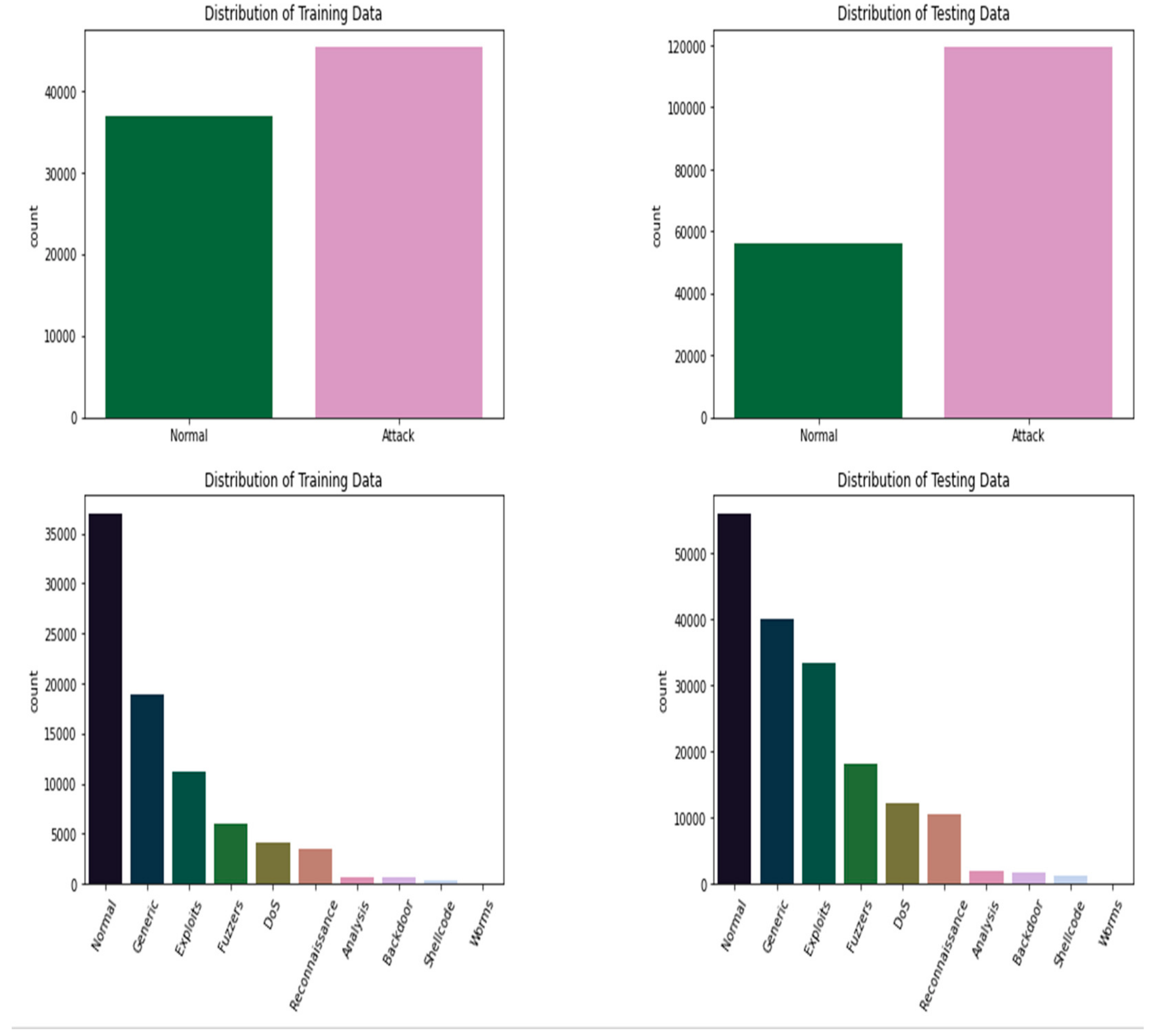
In Figure 2 the x-axis in all the bar graphs shows the captured normal attack patterns and represents nine different attacks as Normal, Generic, Exploits, Fuzzers, Denial of Services, Reconnaissance, Backdoor, Shellcode and Worms, where the y-axis represents the count of the number of records in Figure 2.

The distribution of the training dataset and testing dataset on the basis of different types of normal and attack behaviors is represented in Figure 2.

4. Traditional Regression Analysis

Regression is the methodology to find the functional relation between two or multiple variables. The way the straight line fits over the variables defines the linear regression.

The fitted line equation, which shows the average relationship between two variables and the predicted P value of the dependent variable for the given Q value of the variable, is in Equation (1) [8].

X = p + qY,

(1)

where X and Y are dependent and independent variables, p is bias and Error Rate is X, actual points—X. The error is the difference of points from the line.

For example, if we have values for two variables, say P and Q, and it is needed to fit a line over the top of the points P and Q, and if it is required to check how these points are fitted to the line, then we compute the error value, as in Equation (2) [9]

Error Value = X_actual − X,

(2)

The error is the distance between the fitted line and the point. Here, for the second entry and third entry we get the error of 1 and −1.

To remove the negative entries so that the overall result will not be zero or wrong, we will square the error values. The line is the best fit if the magnitudes of deviations are low for an individual case, for large values of deviation the method of “least squares” is used to minimize the squared deviation in Equation (3) [8].

Thus, for minimization,

$$\sum {\left(y-Y\right)}^2$$

(3)

where y is the variable value and Y is the line. For the coefficients of the least square regression, the line equation a and b is given by Equations (4) and (5) [3,8].

$$\sum y=M\mathrm{a}+\mathrm{b}\sum x$$

(4)

$$\sum xy=\mathrm{a}\sum x+\mathrm{b}\sum x^2$$

(5)

Here, M includes the total number of cases (Equations (4) and (5) are “normal equations”) for simplification [8,26],

$$\mathrm{b}=\frac{\sum xy-\frac{(\sum x) (\sum y)}{M}}{\sum x^2-\frac{{\left(\sum x\right)}^2}{M}},$$

(6)

$$\mathrm{a}=\frac{\sum y}{M}-\mathrm{b}\frac{\sum x}{M}.$$

(7)

If the line passes through (x, y),

$$\mathrm{b}=\frac{\frac{\sum xy}{M}-\overline{x\overline{y}}}{\frac{\sum x^2}{M}-\overline{x^2}},$$

(8)

Here, the denominator is a variance of the variable x, and the numerator is defined as the covariance of the variables x and y. This shows the line of the least squared deviation and shows the manner in which the regression line fits on x, using Equations (6)–(9) [8].

$$\mathrm{a}=\overline{y}-b\overline{x},$$

(9)

The Equation (8) relation between variance and covariance is written as Equation (10) [6,8].

$$\mathrm{b}=\frac{cov\left(x,y\right)}{var x},$$

(10)

The value of the x variable is predicted by using the given value for the y variable, which is represented as the regression of x on y and the equation becomes,

x = a + by.

The xy with b shows the slope of the regression line for x on y. Similarly, the yx with b shows the slope of regression for y on x. The equation b_xy is given as Equations (11)–(13) [20].

$$\mathrm{b}{\mathrm{xy}}_{}=\frac{cov\left(x,y\right)}{var y},$$

(11)

The regression analysis for grouped data follows the same procedure as for the simple linear regression for two variables, apart from the criteria that all the data items that fall into one group are approximated to have a value equal to the mid-point value of a specified group where the data are organized in a two-way matrix, as in Equation (12).

$$\mathrm{b}{\mathrm{yx}}_{=}\frac{\frac{\sum fxy}{M}-\frac{\sum fx}{M} ·\frac{\sum fy}{M}}{\frac{\sum f{x}^2}{M}-(\frac{\sum fx}{M}{)}^2},$$

(12)

Here, the numerator is the frequency and the count of those items which have their values in the specified group for the term variables x and y.

$$=\frac{\frac{\sum f{d}_x{d}_y}{M}-\frac{\sum f{d}_x }{M} \frac{\sum f{d}_y}{M}}{\frac{\sum f{d}_x^2}{M}-\left(\frac{\sum f{d}_x}{M}\right)},$$

(13)

Linear Regression is a supervised learning based algorithm which targets prediction values considering independent variables that define the relationship between multiple variables and forecasting.

The relationship between multiple variables and forecasting and the relationship between dependent and independent variables differ the regression model. The dependent variable (s) is predicted by a given independent variable (t) to define a linear relationship between (s-input) and (t-output). For linear regression, the hypothesis function is given in Equation (14) [20,27]

$$\mathrm{t}={\propto }_1+{\propto }_2\times s,$$

(14)

Here, p is a univariate input training data and q is the data labels. The regression training model should fit a line to predict the data labels for a particular value of one input variable.

The model fits the best when the accurate value of $\propto$₁ and $\propto$₂ is computed, it predicts the value of q on the basis of input value p. The best fit values of $\propto$₁ and $\propto$₂ is computed or updated by using a cost function. To achieve the best fit, the regression model objects to predict data labels (q) in such a way that the difference between the true value and predicted value is minimum. The cost function is used for updating the best fit values of $\propto$₁ and $\propto$₂ to minimize the error rate using Equations (15)–(17) [11,12].

$$\mathrm{mini}\frac{1}{n}{\sum }_{k=1}^n(preditio{n}_{\mathrm{k}}-{\mathrm{q}}_{\mathrm{k}}{)}^2,$$

(15)

$$\mathrm{M}=\frac{1}{n}{\sum }_{k=1}^n(predictio{n}_{\mathrm{k}}-{\mathrm{q}}_{\mathrm{k}}{)}^2,$$

(16)

$$\mathrm{RMSEV}=\sqrt{\frac{{\sum }_{k=1}^n{({\mathrm{q}}_{prediction,k}-{\mathrm{q}}_{\mathrm{k}})}^2}{k}},$$

(17)

Here the root mean square of the difference of the (q) predicted value and the (q) real value is the cost function (M). The cost function is to calculate the difference in the true value and predicted value. Root Mean Squared Error Value is defined by the square root of the mean of the error value square.

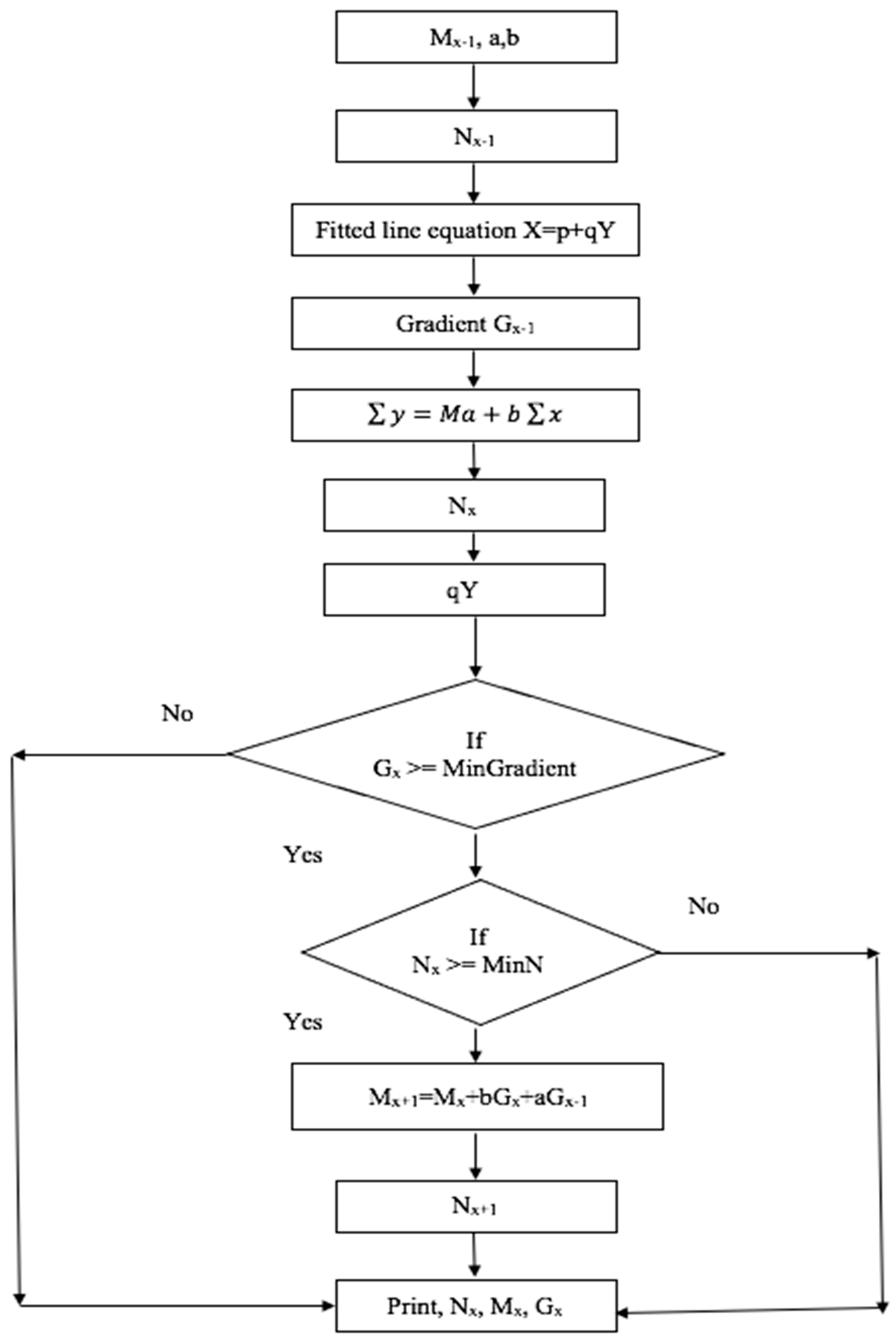
The Figure 3 represents the HNADAM-SDG flow chart, having a tendency to lower itself during convergence, and is represented using variable momentum and a step size, as in Equation (18) [5].

$${\mathrm{M}}_{\mathrm{ij}}(\mathrm{k}+1)={\mathrm{M}}_{\mathrm{ij}}\left(\mathrm{k}\right)+∆{\mathrm{M}}_{\mathrm{ij}}\left(\mathrm{k}\right)+\beta ∆ {\mathrm{M}}_{\mathrm{ij}}(\mathrm{k}-1),$$

(18)

Here, N is the error function, M_{ij the} weight, and $∆$M_ij is the continuous change in the value of the weight for each loop. The objective is to minimize the gradient of N by following the methodology in Figure 3.

5. Proposed Hyperparameter Optimization Algorithm

Linear regression is used to measure the relationship between the population of variables based on collected paired samples. The correlation of variables is determined to further compute the mathematical relationship to predict the value of one variable from the other variable, and to observe the change in the value of variable.

Let the study variable be ‘p’ and explanatory variable be ‘q’, the items for variable ‘p’ and ‘q’ are paired as, (q₁, p₁), (q₂, p₂),……, (q_m, p_m), the simplest form of relation is a linear relationship which is defined as p = x + yq, the line is required to fit along the points. To make the line fit best, the values of a and b are to be maintained accurately.

The least square estimation is made for the best fit of the variables. The exact relation between the variables is found by approximating the relationship along the line, so the line equation can be rewritten as $\overline{p}=x+yq$. Here, $\overline{p}$ is the predicted or estimated value of p. The exact relationship among the variables is defined as p= x+yq=error, the error here is the difference between the predicted value and actual value for (q₁, p₁), (q₂, p₂), ……, (q_m, p_m), the error is computed as (p_j − q − xq_j) for I = 1, 2,…., n, to find the values of a and b, for which the difference is the minimum for the best fit.

In the least square estimation, the summation of the squared residuals is the minimum. The differentiation is separately obtained for a and b, having derivative to be zero. The a and b estimates are defined in Equations (19)–(21) [5].

$$\widehat{a }=\overline{y}-\widehat{b}\overline{x},$$

(19)

$$\widehat{y}=\frac{{\sum }_{j=1}^m\left(a_j-\overline{a}\right)\left(b_i-\overline{b}\right)}{{\sum }_{i=1}^n(a_i-\overline{a{)}^2}}=\frac{SSXY}{SSX},$$

(20)

The least square estimation (LSE) r for b is,

$$\mathrm{r}=\widehat{y}\sqrt{\frac{{\sum }_{b=1}^m{(q_i-\overline{q})}^2}{{\sum }_{j=1}^m{(p_i-\overline{p})}^2}}=\widehat{y}\sqrt{\frac{SSX}{SSY}},$$

(21)

Here r and $\widehat{y}$ are same. Coefficient of determination is used when there is no linear relationship between the variables, the residual quantities are as in Equation (22) [11].

$$p_i-x-y{q}_{j },\mathrm{where}(\mathrm{j}=1,2,\dots \dots ,\mathrm{m})$$

(22)

The fitted linear model has a small magnitude of the residuals, the variability of Y using X shows how the change in the values of Y affects the prediction of the values. The variance is computed as in Equations (23)–(30) [11].

$$\frac{1}{m}{\sum }_{j=1}^m{(p_i-\overline{p})}^2,$$

(23)

this is partitioned as,

$$\frac{1}{m}{\sum }_{j=1}^m{(p_j-\overline{p})}^2=\frac{1}{m}{\sum }_{j=1}^m{(p_j-\widehat{p_j}+\widehat{p_j}-\overline{p})}^2=\frac{1}{m}{\sum }_{j=1}^m{(p_j-{\widehat{p}}_j)}^2+\frac{1}{m}{\sum }_{j=1}^m{(\widehat{p_j}-\overline{p})}^2,$$

(24)

$${\sum }_{j=1}^m{(p_j-\overline{p})}^2={\sum }_{j=1}^m{(p_j-\widehat{p_j})}^2+{\sum }_{j=1}^m{(p_j-\overline{p})}^2,$$

(25)

$$\frac{1}{m}{\sum }_{j=1}^m\left(p_j-\widehat{p_j}\right)\left(\widehat{p_j}-\overline{p}\right)=0,$$

(26)

Here $p_j-\widehat{p_j}$ is the residual.

The sum of the squares due to errors (SSE) is defined as

$${\sum }_{j=1}^m{(p_j-\widehat{p_j})}^2,$$

(27)

The sum of the squares due to regression (SSR) is given as

$${\sum }_{j=1}^m{(\widehat{p_j}-\overline{p})}^2,$$

(28)

The total variability in p is,

$$\mathrm{P}(\mathrm{SST}=\frac{1}{m}{\sum }_{j=1}^m{(p_j-\overline{p})}^2),$$

(29)

R² = SSR/SST = 1 − (SSE/SST),

(30)

0 $\le R^2\le 1$, when R² is near to 1, and then it is to be found that most of the variability falls in y and the model is the best fit, and when R² is close to 0 then it defines that there is not much variability in Y and the model is not a good fit.

The variability of Y values around the predicted regression line is measured by estimating the standard error as S_pq = $\sqrt{\frac{SSE}{m-2}}$, when the predicted outcome is close to the observed values then the standard error is less, for the hypothesis as in Equation (31)–(34) [9,28].

$$\mathrm{H}\alpha \left(A\right)={\propto }_0+{\propto }_{1}A,$$

(31)

We need to fit, for the training data, and so the cost function is used as the mean squared error:

$$\mathrm{Mean}\mathrm{Squared}\mathrm{Error}=\frac{1}{k}{\sum }_{j=1}^k{(q_j-q_{vector j})}^2,$$

(32)

This error is minimized by using a gradient descent optimization algorithm, such as:

$${\propto }_k={\propto }_k-\theta \frac{\partial }{\partial {\propto }_k} B\left({\propto }_0, {\propto }_1\right) for k=0 and k=1,$$

(33)

The testing of the hypothesis using a correlation coefficient along the slope is given by the test statistic,

$$T_c=\frac{\widehat{b}}{\sqrt{\frac{SSE}{\left(n-2\right)SSX}}},$$

(34)

testing the hypothesis H_o where b = 0 and H_a $where b\ne$ 0.To predict the Y value using the fitted line, the confidence interval and prediction interval are used, which defines the point of estimation of the population.

The confidence interval is shown in Equation (35) [9].

$$\widehat{p_j} \pm s_{\propto /2} \left(d.f.=m-2\right)S_{pq}\sqrt{\frac{1}{m}+\frac{{(q_{j-}\overline{q})}^2}{SSX}},$$

(35)

The prediction interval is shown in Equation (36) [26].

$$\widehat{p_j} \pm s_{\propto /2} \left(d.f.=m-2\right)S_{pq}\sqrt{1+\frac{1}{m}+\frac{{(q_{i-}\overline{q})}^2}{SSX}},$$

(36)

To define the individual variable value, the defined value must be obtained using a prediction interval.

The gradient descent algorithm uses the gradient of function parameters to identify the search space. HNADAM-SDG is based on the NADAM Nesterov Momentum version of gradient descent. Hypertuning is used for attaining the betterment of performance. This algorithm follows the negative values of objective parameters to relocate the minimum of function. It measures the displacement in weight with respect to the displacement in error. The gradient is also understood as the function of a slope. The gradient is inversely proportional to the steepness of the slope. The learning of the model depends on the steepness of the slope. If the slope tends to zero, then the model stops learning, which is given by Equations (37)–(49) [29].

$$\overline{p}=nq+b,$$

(37)

$$\mathrm{Error}=\overline{p}-p,$$

(38)

$${\mathrm{Error}}^2\left(\mathrm{Cos}\mathrm{t}\mathrm{Function}\right)=\mathrm{Estimated}\mathrm{Value}-\mathrm{Actual}\mathrm{Value}=({(\overline{p}-p)}^2,$$

(39)

L.F = ((nq + b) − b)², loss function = L.F,

(40)

L.F = ((nq + b) − p)²,

(41)

L.F = f(n,b),

(42)

$$\mathrm{Total}\mathrm{Loss}=\mathrm{T}.{\mathrm{L}}_{\mathrm{Total}}=\frac{1}{M} {\sum }_{j=1}^M{(\left(n_j+b\right)-p_j)}^2,$$

(43)

$$\frac{\partial s}{\partial n}=\frac{\partial }{\partial b}{({\sum }_{j=1}^M\left(n{q}_j+b\right)-p_j)}^2),$$

(44)

$$\frac{\partial s}{\partial b}=\frac{\partial }{\partial b} ({\displaystyle \sum }_{j=1}^M((n{q}_j+b)-p_j{)}^3),$$

(45)

The gradient descent with respect to “b”

$$\frac{\partial }{\partial b}=\frac{\partial }{\partial b} ({\sum }_{j=1}^M((n{q}_j+b)-p_j{)}^2),$$

(46)

$$\frac{\partial }{\partial b}=2 ({\displaystyle \sum }_{j=1}^M((n{q}_j+b)-p_j))$$

(47)

The gradient descent with respect to “n” is given by Equations (48) and (49) [29,30].

$$\frac{\partial s}{\partial n}=\frac{\partial }{\partial n} ({\sum }_{j=1}^M((n{q}_j+b)-p_j{)}^2),$$

(48)

$$\frac{\partial s}{\partial n}=2 ({\displaystyle \sum }_{j=1}^M((n{q}_j+b)-p_j))$$

(49)

Experimental Analysis

The UNSW-NB15 dataset comprises 254,004 attacks of data, categorized as normal and attack. A total of 49 features were there [32], including flow and packed based features from data packets. Attacks were categorized into different classes, such as normal, analysis, backdoor, DoS, Exploits, Fuzzers, Worms, Generic, Shellcode and Reconnaissance [33]. The list of features selected for experimental analysis is presented in the

Table 1. Selected Features.

S.No.	Feature Name	Description
1	Proto	Protocol
2	Dur	Duration
3	State	State Protocol
4	Service	Services by Network
5	Spkts	Source to Destination Packet Count
6	Dpkts	Destination to Source Packet Count
7	Sbytes	Transaction Bytes Source to destination
8	Dbytes	Transaction Bytes Destination to Source
9	Rate	Data Rates
10	Sttl	Source to destination Time to Live Value
11	Dttl	Destination to source Time to Live Value
12	Sload	Source Bits per second
13	Dload	Destination Bits per second
14	Sloss	Source packets retransmitted or dropped
15	Dloss	Destination packets retransmitted or dropped
16	Sinpkt	Source interpacket arrival time (mSec)
17	Dinpkt	Destination interpacket arrival time (mSec)
18	Sjit	Source jitter (mSec)
19	Djit	Destination jitter (mSec)
20	Swin	Source TCP window advertisement value
21	Stcpb	Destination TCP window advertisement value
22	Dtcpb	Destination TCP base sequence number
23	Dwin	Destination TCP window advertisement value
24	Tcprtt	TCP connection setup round-trip time

.

The HNADAM-SDG algorithm (Algorithm 1) is employed over the dataset with the list of selected features. The complexity of the algorithm (Algorithm 2) is determined by computing the sum of all the gradients to lower the computation cost per iteration with the convergence of necessary iterations. The algorithm adopts the methodology to uniformly select the observation as n and used the estimator function f(s) as f_n(s).

Algorithm 1: HNADAM-SDG

Initialize “m” and “c” in the start with a random number.

Calculate gradient.

Update the calculated gradient with respect to “m” and “c” using Equations (50)–(52) [31].

$$\frac{\partial s}{\partial n}=\frac{\partial }{\partial n} ({\sum }_{j=1}^M((n{q}_j+b)-p_j{)}^2),$$ (50)

$$\frac{\partial s}{\partial n}= 2 ({\sum }_{j=1}^M((n{q}_j+b)-p_j))$$ (51) ,

The learning rate is multiplied by “n” and “b”.

Update the value of “n” and “b” for every step.

The class-conditional densities are not being modeled in the logistic discrimination:

Model Parameter β

Parameter Initialization,

Normal distribution $\beta ~M\left(Q,{\theta }^2\right)$

Initial vector n = 0,

Initial vector u = 0,

Initial steps T = 0

Initial convergence parameter as Boolean = F,

While Boolean = = F,

Do shuffle the training set T for each mini-batch $\mathrm{b}\subset T$ and do the update step T = T + 1

Compute the gradient vector $\mathrm{G}={\nabla }_{\beta }\mathcal{L}\left(\beta ;b\right)$ on the mini-batch b.

Update Vector n.

$\mathrm{m}={\alpha }_1.n+\left(1-{\alpha }_1\right).G$

Update Vector $n={\alpha }_2.u+\left(1-{\alpha }_2\right).GʘG$

Rescal Vector $\exists =\frac{\mathrm{n}}{1-{\alpha }_1^T}$

Rescal Vector $\mathrm{U}=\mathrm{U}/\left(1{\alpha }_2^T\right)$

Update Variable in Equation (52) [29]

$$\beta =\beta -\frac{m}{\sqrt{u+x}} ʘ\left({\alpha }_{1}m+\frac{\left(1-{\alpha }_1\right)}{1-{\alpha }_2^T} .G\right),$$ (52)

End for

If convergence condition holds then

Boolean = T

End if

End while

Return model variable β

The iterative loop, For i = 0,------,c

$P_i\leftarrow rand\left(-0.10, 0.10\right)$ to compute random variable ranging between −0.10 to 0.10

The iteration is made:

Repeat

For i = 0,-----,

$∆P_i\leftarrow 0$

For i = 0,-----,c

$0\leftarrow 0+P_i{A}_i^T$

$B\leftarrow sigmoid\left(0\right)$

$∆P_j\leftarrow ∆P_j+\left(R^T-B\right)A_i^T$

For j = 0,-----,d

$P_i \leftarrow P_i+n∆P_i$

Until convergence repeat the iteration

The iterative loop For j = 1,----,v

For i = 0,----,c

$P_{ij}\leftarrow rand\left(-0.10,0.10\right)$

The iteration is made using

Repeat

For j = 1,----,v

For i = 0,----,c

$∆P_{ij}\leftarrow 0$

For T = 1,----,m

For j = 1,-----,v

$Q_i \leftarrow 0$

For i = 0,-----,c

$Q_i\leftarrow Q_i+P_{ij}{A}_i^T$

For i = 1,-----,v

$B_j\leftarrow exponential\left(Q_i\right)/{\mathsf{\Sigma }}_{\upsilon } exponential\left(Q_{\upsilon }\right)$

For j = 1,-----,v

For i = 0,-----,c

$∆P_{ij}\leftarrow ∆P_{ij}+\left(R_i^T-B\right)x_j^T$

For j = 1,-----,v

For i = 0,-----,d

$P_{ij}\leftarrow P_{ij}+n∆P_{ij}$

Repeat the iteration until convergence.

Training T; Learning Rate N; Normal Distribution θ; Decay Parameters α1, α2

Algorithm 2: Complexity Computation

Initialize the weights as s1

For m = 1 to M do

Observation of sample n uniformly as random in Equation (53) [29].

$${\mathrm{s}}_{\mathrm{m}+1}\leftarrow {\mathrm{s}}_{\mathrm{m}}-\mathbf{\beta }\nabla {\mathrm{f}}_{\mathrm{s}}\left({\mathrm{s}}_{\mathrm{m}}\right),$$ (53)

end for

wM return.

This holds O(n) computations, as the number of iterations (i) is larger in the testing and training of the sampled dataset. The computation cost is determined, as defined in

Table 2. Complexity of HNADAM-SDG algorithm.

Method	Iterations	Per Iteration Cost	Total Cost
HNADAM-SDG	$\mathrm{O}(1/\in )$	O(i)	$\mathrm{O}(\mathrm{i}/\in )$

.

The computation cost of HNADAM-SDG is better and more efficient as it shows linearity for the different training sets. If the matrix size is (p,q), then the total cost would be O(kpq), where k denotes the number of epochs and q is the number of attributes per sample, which is not zero.

6. Results and Discussion

The performance of the HNADAM-SDG algorithm is compared with logistic regression, ridge classifier and ensemble techniques. The UNSW-NB15 training and testing data is used for training and testing of the IDS model on the basis of occurrences of attacks. The performance measures are accuracy and error rate that are driven from the confusion matrix.

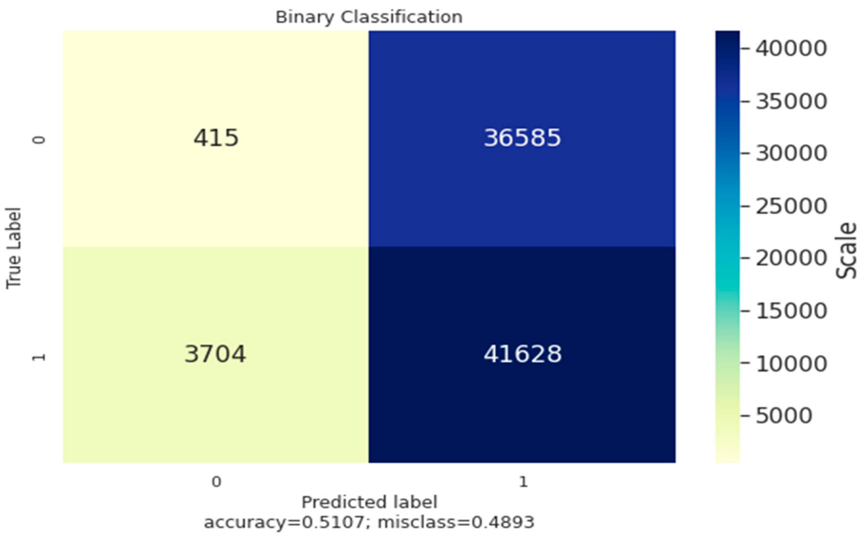
The Figure 4 shows the classification of data using the confusion matrix, which is a two by two matrix consisting of outcomes produced by a binary classifier as the overall accuracy, error-rate, sensitivity, precision and specificity. The binary classifier produces results, with labels such as 0/1 and Yes/No. The instances of all the test data is predicted using the classifier as true positive, true negative, false positive and false negative. The matrix derives the error rate and accuracy as the primary measure. Here, the confusion matrix computes the accuracy as 0.51 and error rate as 0.489; the matrix is built between the true label and predicted label, with labels such as 0/1, and having a data scale.

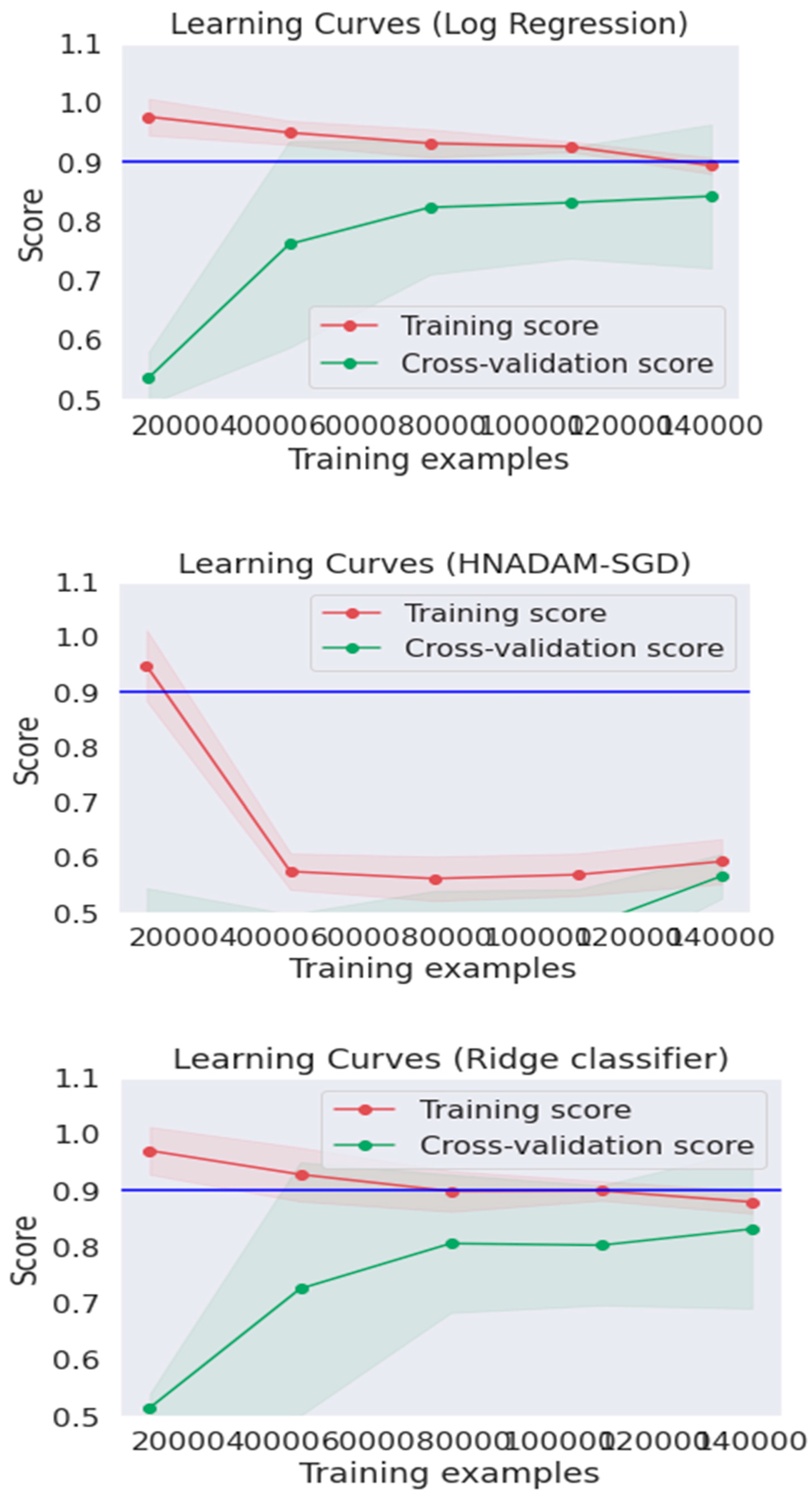
The Figure 5 shows the learning curves for logistic regression, ridge classifier and HNADAM-SDG techniques. The learning curve is measured by taking samples from a training dataset to measure a model of performance by computing the error rate over a validation dataset. The best fit algorithm has a zero error rate to fit the data points. The error rate of the model varies as the size of the training instance fluctuates. The curve shows the change in error, training score and cross validation score as the training instance changes.

The

Table 3. Performance Matrix.

Logistic Regression
	Precision	Recall	F1-Score	Support
0	0.48	0.82	0.61	3971
1	0.99	0.96	0.98	78,361
Accuracy			0.96	82,332
Macro Average	0.74	0.89	0.80	82,332
Weighted Average	0.98	0.96	0.96	82,332
Ridge Classifier
	Precision	Recall	F1-Score	Support
0	0.70	0.72	0.71	3971
1	0.99	0.98	0.98	78,361
Accuracy			0.98	82,332
Macro Average	0.85	0.86	0.85	82,332
Weighted Average	0.98	0.98	0.98	82,332
HNADAM-SDG
	Precision	Recall	F1-Score	Support
0	0.71	0.70	0.71	3971
1	0.99	0.98	0.99	78,361
Accuracy			0.99	82,332
Macro Average	0.87	0.88	0.86	82,332
Weighted Average	0.98	0.98	0.98	82,332
Ensemble
	Precision	Recall	F1-Score	Support
0	0.49	0.80	0.60	3971
1	0.98	0.98	0.98	78,361
Accuracy			0.97	82,332
Macro Average	0.76	0.88	0.86	82,332
Weighted Average	0.98	0.96	0.97	82,332

represents the performance measures for different algorithms such as logistic regression, ridge classifier, HNADAM-SDG and Ensemble techniques, applied over the dataset to predict the emerging attack patterns. The performance is measured by computing precision, recall, F1-score and the support value for the 0/1, macro average, accuracy and weighted average.

The

Table 4. Time Complexity Analysis.

Processing Time
S.No.	Algorithms	Training Time (Second)	Testing Time (Second)
1.	Logistic Regression	500.23	15.23
2.	Ridge Classifier	450.50	14.56
3.	HNADAM-SDG	300.30	12.42
4.	Ensemble	780.48	20.31

represents the processing time for various algorithms on the basis of the training and testing times for logistic regression, ridge classifier, HNADAM-SDG and Ensemble techniques applied over the dataset to predict the emerging attack patterns.

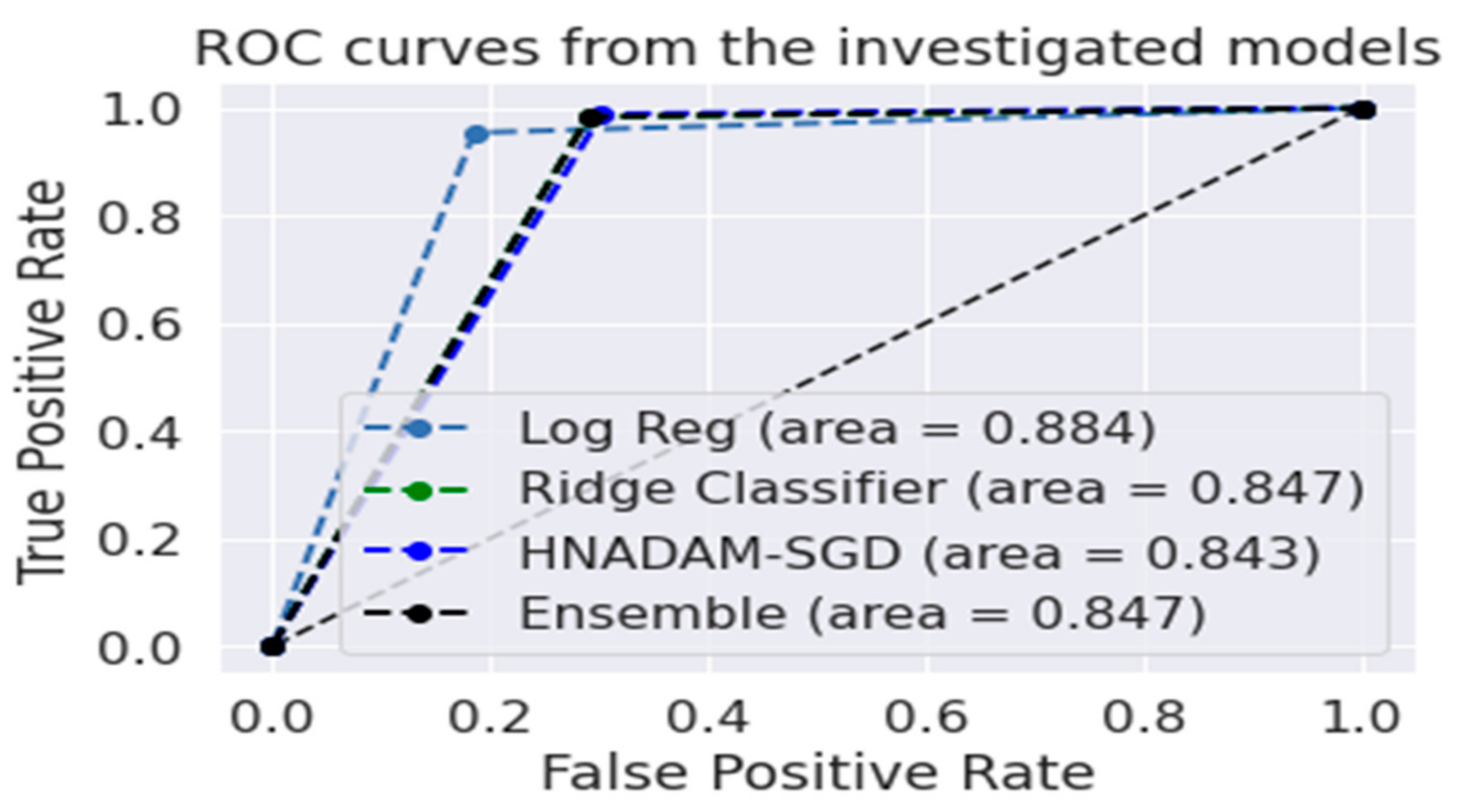
The Figure 6 shows the ROC curve areas for the logistic regression, ridge classifier, HNADAM-SDG and ensemble algorithms to find the area under the curve of the receiver characteristic operator (ROC) to find plots denoting TPR and FPR, considering the threshold value, by obtaining the probability curve to separate the signal from the noise. The higher value of the area under the curve represents the better performance of the algorithm.

AUC = 1 denotes that all positive and negative classes are pointed correctly using a classifier.

0.5 < AUC < 1 shows that the chance of distinguishing between positive and negative classes is higher.

AUC = 0.5 shows that the classifier is not able to distinguish between positive and negative classes.

The higher value of the X-axis shows the higher number of false positives, while the Y-axis shows the higher number of true positives.

The statistical measures of sensitivity and specificity are used for measuring the performance of the algorithms, which is computed as Equations (54) and (55) as [29]. Here NTP is the total number of true positives, NFN is the total number of false negatives, NTN is the number of true negatives and NFP is the number of false positives.

$$\mathrm{Sensitivity}=\frac{\mathrm{NTP}}{\mathrm{NTP}+\mathrm{NFN}},$$

(54)

$$\mathrm{Specificity}=\frac{\mathrm{NTN}}{\mathrm{NTN}+\mathrm{NFP}},$$

(55)

The

Table 5. Performance Analysis.

Performance Analysis
	Algorithms	Accuracy	Sensitivity(s)	Specificity
1.	Logistic Regression	0.967	0.955	0.971
2.	Ridge Classifier	0.986	0.961	0.989
3.	HNADAM-SDG	0.998	0.977	0.995
4.	Ensemble	0.977	0.957	0.963

shows the performance analysis for the comparison of the performance of different algorithms applied over the dataset. The accuracy, sensitivity and specificity represent the best fit model for testing and training.

7. Research Limitations

• The hyperparameter optimization algorithm performance depends on various factors such as total hidden layers, total per-layer units, dropout amount, the regularizer learning rate and weight decay.
• The non-optimal setting of hyperparameters will drastically affect the algorithm’s performance, that varies from extremely a low learning rate to a very large learning rate.
• The hypertuning approach varies depending upon the type of dataset, the nature of the dataset, and its size as there is no well-defined formula to find hyperparameters.
• The criticality is to choose what number of parameters are going to be tested, due to which performance gets affected by the extremely low learning rate of (1 $-$ e⁻⁵) or the very large learning rate of 10, by opting for the wrong hyperparameters.
• There exists no well-defined formula to find hyperparameters as it depends on the algorithm type, the dataset and the dataset size.
• The performance of the algorithm varies with the change in the dataset’s parameters.

8. Conclusions and Future Scope

In this paper, the IDS model is determined using the hybridization of the HNADAM-SDG algorithm. The performance of the algorithm is compared with other classification algorithms by adapting feature selection and optimization techniques. The algorithm is used for testing and training of the UNSW-NB15 dataset. The HNADAM-SDG techniques are used to measure the relationship between the population of variables based on collected paired samples. The correlation of variables is determined to further compute the mathematical relationship, to predict the value of one variable based on another variable, and to observe the change in the value of variables. The best fit algorithm has a zero error rate to fit the data points. The error rate of the model varies depending on the size of the training samples. The performance is visualized using learning curves and AUC-ROC curve areas. In the future, the IDS will help in mitigating the impact of malicious activities over emerging information sharing platforms. The IDS will evolve in diversified research areas such as,

• The IDS for Internet of Things (IoT), which is the booming area for attackers. This includes breaching security of automotive, wearable and connected devices.
• The IDS for cyber insurance, which is the upcoming ideology to receive attention to mitigate the damages from upcoming data losses, sabotage and theft events.
• The IDS for analyzing the effectiveness of nature inspired optimization algorithms over the latest datasets, such as CCIDS and streaming datasets.