Data Preprocessing Combination to Improve the Performance of Quality Classification in the Manufacturing Process

Abstract

The recent introduction of smart manufacturing, also called the ‘smart factory’, has made it possible to collect a significant number of multi-variate data from Internet of Things devices or sensors. Quality control using these data in the manufacturing process can play a major role in preventing unexpected time and economic losses. However, the extraction of information about the manufacturing process is limited when there are missing values in the data and a data imbalance set. In this study, we improve the quality classification performance by solving the problem of missing values and data imbalances that can occur in the manufacturing process. This study proceeds with data cleansing, data substitution, data scaling, a data balancing model methodology, and evaluation. Five data balancing methods and a generative adversarial network (GAN) were used to proceed with data imbalance processing. The proposed schemes achieved an F1 score that was 0.5 higher than the F1 score of previous studies that used the same data. The data preprocessing combination proposed in this study is intended to be used to solve the problem of missing values and imbalances that occur in the manufacturing process.

1. Introduction

Recently, interest in the “smart factory” has been increasing for the improvement of manufacturing competitiveness, and with the development of information and communications technology (ICT), manufacturing companies are making great efforts to increase production efficiency by analyzing data that can be collected during the manufacturing process. As the application of sensing technology is increasing, the amount of data collected during the manufacturing process is also constantly increasing.

Machine learning and deep learning are being used as methods to uncover meaningful information about process states from the big data of complex manufacturing processes, and they are often used to explore important variables for quality improvement or information that determines quality. In this case, good performance is achieved when the collected data are sufficiently large and the classes are evenly distributed. However, there are sometimes missing values in the sensor data collected for equipment failure, maintenance, and the repair of equipment [1], and missing values in the data obtained in real time affect the final performance of machine learning models [2]. In addition, during the manufacturing process, a data imbalance can occur when there are many samples of good products and insufficient data for samples of defective products. In the case of a dataset with an imbalanced class, the model does not learn properly on the entire dataset, but is biased to a large number of classes, which causes problems in data analysis [3]. For example, because most of the class variables for the data used in the quality classification model are good products, the quality classification model that learns from these data classifies most products as good products. A model trained with imbalanced data classifies most of the results as the majority class, because the decision boundary of the model is biased toward a minority class [4]. As a result, although the overall accuracy of the model is high, a data imbalance occurs where a small number of classes cannot be classified properly.

As many IoT sensors will be attached in the future, it is expected that the problem of missing values and data imbalances in the collected data will continue to occur. In this study, several models are proposed to improve missing data values and data imbalances to obtain meaningful results, such as results for the improvement of quality classification accuracy. To this end, we propose a method that solves the problem of missing values and imbalances in the data and shows the most optimal performance. In particular, by using the data collected from sensors in the semiconductor manufacturing process to improve missing data values and imbalance problems, we intend to obtain meaningful results for an improvement in quality classification accuracy. Therefore, the purpose of this study is to remedy the missing values and imbalances in the collected data using machine learning and deep learning methods for quality control in the manufacturing process and to improve the quality classification performance.

Table 1. Research questions and approaches.

Questions	Approaches
How can missing values in the data be replaced?	Use single and multiple imputation methods to replace missing data
Which methodology can one use to address data imbalances?	Use legacy simple oversampling, hybrid sampling, and a GAN
How does one evaluate the performance of quality classification?	Use the F1 score as an evaluation indicator considering the characteristics of imbalanced data

shows the research questions for this study, and the approaches considered in this study for each question.

This study uses the Semiconductor Manufacturing (SECOM) dataset, which is available from the University of California, Irvine (UCI) machine learning repository. The SECOM dataset contains 1567 instances taken from a wafer fabrication production line in the semiconductor industry. Each instance is a vector of attributes, that is, a timestamp and 590 sensor measurements plus a label for the Pass/Fail test. Some missing values exist. In the case of the Pass/Fail test, which indicates the quality of the semiconductor manufacturing process, −1 means good and 1 means bad. For convenience, in this study, good was set to 0 and bad was set to −1.

This paper is structured as follows. Section 2 reviews the existing literature related to this study, and Section 3 introduces the theoretical background of the methodologies used in this study. In Section 4, the data preprocessing process is explained, and in Section 5, the experiment conducted in this study is explained in detail and the results on the significance of the quality classification performance evaluation and parameters are interpreted. Section 6 summarizes the research results and presents a conclusion.

2. Literature Review

2.1. Machine Learning Studies Using the SECOM Dataset

In several previous studies, various machine learning techniques were used to improve the quality classification performance with SECOM data. Ref. [5] built a model using various techniques, such as support vector machine (SVM), naive Bayes, and decision tree techniques, to predict quality in the semiconductor manufacturing process. They tried to improve the model performance by considering missing values that could occur in data collected in the real world using the SECOM dataset and by studying an efficient method for replacing missing values. Ref. [6] tried to improve the performance of the methodology, and they used the Boruta and MARS methods to find the features most related to model performance and to train the model. Ref. [7] studied the performance improvement of the classification model using random oversampling to select 25% of the highly correlated features using the dataset and to solve the data imbalance problem. Ref. [8] searched for the model with the highest performance by comparing several models, such as decision tree, naive Bayes, and logistic regression models. Ref. [9] applied the synthetic minority oversampling technique (SMOTE) and random undersampling to solve a data imbalance and applied it to some methodologies to improve the model performance.

In previous studies, missing values and data imbalances were partially considered, but the performance of the proposed classification model was low. In this study, a single replacement method and multiple replacement methods were applied to replace missing values, and various methods were applied to solve the data imbalance problem to improve the quality classification performance and propose an efficient data preprocessing method.

2.2. Mutiple Imputation Studies for Missing Data

Ref. [10] proposed an algorithm that enables the improvement of the classification model’s performance by replacing missing values using a weighted distance metric based on mutual information using k-nearest neighbor (KNN). Ref. [11] randomly introduced missing values in 10 open datasets at 10%, 20%, and 30% ratios, and compared them with widely used methods for replacing missing values, such as KNN, multiple imputations by chained equations (MICE), and MissPALasso. They observed the best performance when using MissForest to replace missing values. Ref. [12] found that missing values are generally present in all datasets and studied ways to use KNN, fuzzy k-means, singular value decomposition (SVD), Bayesian principal component analysis (bPCA), and MICE to explore the most efficient way to replace missing values. Ref. [13] trained a model to replace existing missing values with the median, expectation–maximization, and KNN techniques to compare the models’ performance in predicting the survival of breast cancer patients. It was shown that the best results were obtained when missing values were replaced using KNN. Ref. [14] conducted a study to propose an appropriate replacement set for missing values by structuring and classifying missing patterns and applying a probabilistic multiple imputation approach to solve the problem of data replacement in the case of multivariate time series data.

Since most of the existing classification algorithms learn under the assumption that the number of data points belonging to each class is almost the same, when the number of data points in each class is imbalanced, the classification accuracy is somewhat lowered. In this study, to replace missing data that may be caused by the maintenance or breakdown of equipment, the linear interpolation, poly interpolation, KNN, MICE, and MissForest methods were used.

2.3. Data Imblance Studies

There is a specific data sampling technique that is used to resolve data imbalances. Data sampling is a technique for creating a balanced dataset by adjusting the number of samples from the majority class (occupying a large part of the sample) and the minority class (occupying a small part of the sample). Data sampling is divided into an undersampling technique and an oversampling technique, according to which the number of samples is adjusted [15]. Various methodologies have been studied to solve the classification problem in the field of machine learning. However, because most of the existing classification algorithms learn under the assumption that the number of data points belonging to each class is almost the same, the classification accuracy will somewhat lower when the amount of data in the classes is imbalanced. To address these issues, Ref. [16] proposed an oversampling technique to balance the amount of data by learning features belonging to a class with a small amount of data through the application of conditional generative adversarial networks (CGANs), which restrict the learning method through conditions and by generating data similar to real data. In this study, SMOTE, SMOTE-Tomek, SMOTE-ENN, Adaptive Synthetic Sampling (ADASYN), and a GAN were used to improve the model performance to deal with the data imbalance problem.

Table 2. Summary of the literature review.

Author	Algorithm
Lamari et al. [17]	Hybrid sampling method using SMOTE-ENN
Chawla et al. [18]	Combination of methods
Batista et al. [19]	SMOTE-Tomek and SMOTE-ENN
Liang [20]	Hybrid sampling method using bagging
Branco et al. [21]	Research on the imbalanced data problem

summarized the related literatures and their proposed algorithm.

3. Theoretical Background

3.1. Data Imputation Methodology

Linear Interpolation: When the values of two points are given, this method performs a linear calculation according to the straight-line distance to estimate the value located between the points, and it is the simplest method for replacing missing values.

Poly Interpolation: As a generalization of linear interpolation, polynomial interpolation increases the computational complexity of linear interpolation because the degree of the polynomial increases as the number of data points increases. In this study, as a basic methodology for comparison with other methodologies, missing values in the data were replaced for the case of two-degree polynomials.

KNN (K-Nearest Neighbor): This is a method for replacing missing values by classifying the group with the largest number of k elements closest to the analysis target. If the missing value is categorical, it is replaced with the mode of the neighboring data, and if it is continuous, it is generally replaced with the median of the neighboring data. When KNN is used to replace missing values, it can be applied only to independent variables, not dependent variables, and when it is applied to target variables, its predictability decreases.

MICE: Instead of replacing the missing value once, it is replaced while checking the uncertainty of the missing value by replacing it several times. The MICE methodology can be used for both discrete and continuous variables. By using the dataset in which the initial missing values exist, several similar datasets with the replaced values are created. After estimating the propensity score through generalized boosted modeling (GBM) on a similar dataset, a final alternative dataset is provided using the weighted regression analysis of propensity scores to derive summed estimates according to Rubin’s rules.

MissForest: Using this method, it is possible to replace missing values in numerical and categorical variables, and the response to outliers is insensitive. Using each variable and response variable, a random forest is trained to obtain a predicted value.

3.2. Methodologies for Handling Data Imbalances

SMOTE: This is an oversampling method that takes a sample of a class with a small number of data points, finds k neighbor data samples, and generates a random value between the samples to create and add a new sample. There is no data loss, and the overfitting caused by simply duplicating the values of a minority class is alleviated compared with when random oversampling is performed. Bootstrapping or KNN techniques are used, and it is the most-used method for generating synthetic data among the oversampling methods. It has the disadvantage of being weak in predicting data for new cases.

SMOTE-Tomek: TomekLinks are a pair of data points belonging to different classes, when there are no other data points that are closer to each other. As shown in Figure 1b, if two data points of different classes are very close together, they become TomekLinks. It is a method for finding close pairs of data points and then removing from the pairs the data belonging to the majority class. Because this introduces the problem of data loss, it is necessary to exercise care in its application. However, by removing multiple classes, the data imbalance problem can be solved, and, at the same time, as the distance between the two classes increases, the boundary line is pushed toward the multiple classes, making the classification problem easier.

SMOTE-ENN: In the ENN method, if the majority class of the observation’s KNN and the observation’s class are different, then the observation and its KNN are deleted from the dataset. This causes the majority class data around the minority class to disappear. Therefore, the distinction between the minority class and the majority class becomes relatively clear because all data having a minority class among the KNNs are removed.

ADASYN: This method was proposed to solve the overfitting problem of SMOTE and to control the amount of synthesized data in order to more systematically generate them according to the distribution of the surrounding data [22]. ADASYN generates synthetic data according to the density of the data, and the synthetic data generation is inversely proportional to the density of the minority class. A lot of synthetic data are generated when there are few classes that are less dense.

GAN: A GAN is a deep learning model, as shown in Figure 2, that consists of a generator that generates virtual data based on the data distribution and a discriminator that separates the generated data from the real data. The generator receives the z value at random, generates a sample, and trains it to be similar to the real data so that it can be judged as real data. The discriminator trains the generated data through the real data to be able to distinguish it from the real data. The generator and discriminator learn in such a way that they compete with each other for opposite purposes, and when the discriminator cannot distinguish between real data and generated data, the learning procedure ends.

3.3. Machine Learning Classification Methodologies

Logistic Regression: This is a supervised learning model that predicts the probability that data will belong to a certain category as a value between 0 and 1 and classifies it as belonging to one or the other category according to the probability.

Decision Tree: This is a supervised learning model that classifies data according to specific criteria and splits the variable area into two for each branch. As a non-parametric model, assumptions such as linearity, normality, and equal variance are not required. However, because continuous variables are treated as discontinuous values, the probability of prediction errors near the boundary of separation is high, and because the continuous variables depend only on the training data, there is a high probability of instability in the prediction of new data.

Random Forest: This is a model for addressing the tendency of overfitting to the training data that occurs in decision trees. A random forest is constructed through multiple decision trees, characteristic data values are repeatedly selected from a data sample, and the most frequent prediction results are selected using multiple decision trees to determine the final prediction value.

SVC(Support Vector Classification): This is a predictive model that has been actively used since the late 1990s after it was proposed by [23]. Given a set of data belonging to one of two classes, the algorithm finds the boundary with the largest width as a criterion to determine which class the new data belong to. Linear classification and non-linear classification are possible, and there are not many parameters to consider when creating a model. A model can be created even with a small amount of data, and before deep learning was used, it was considered to be the most technologically advanced model among the classification models.

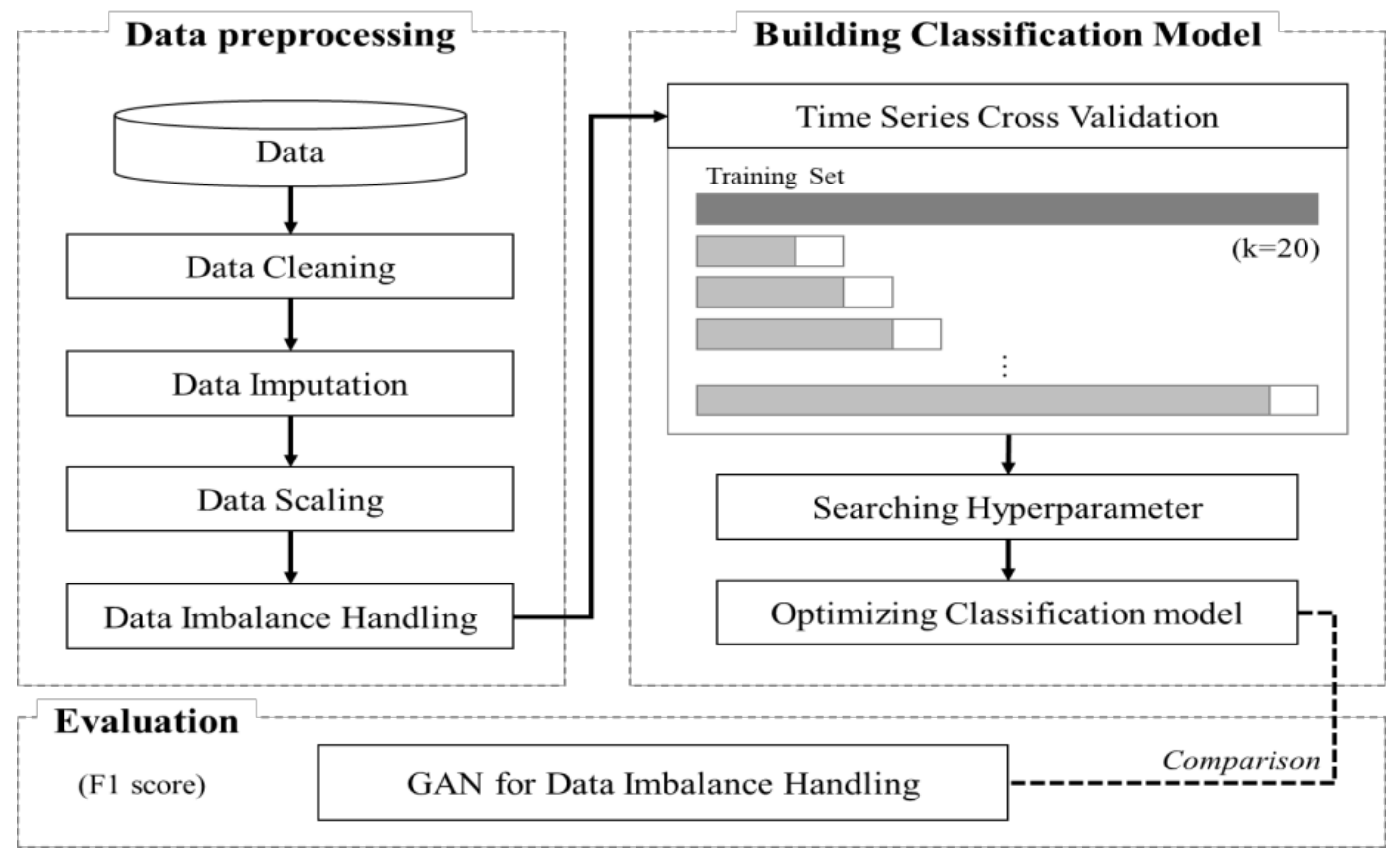
4. Proposed Methodology

The proposed methodology of this study involves three stages: Data Preprocessing, Building a Classification Model, and Evaluation, as shown in Figure 3. “Data Preprocessing” proceeds with Data Cleaning, Data Imputation, Data Scaling, and Data Imbalance Handling. “Building a Classification Model” proceeds with Time Series Cross Validation, Searching for Hyperparameters, and Optimizing the Classification Model. Finally, “Evaluation” tries to find the optimal classification performance and combination of data preprocessing procedures relative to the GAN used to deal with the imbalance.

4.1. Data Preprocessing

4.1.1. Data Cleansing

Columns with missing values and single values were removed before the preprocessing and analysis were performed. First, as shown in

Table 3. Ratios of missing values in the dataset.

Ratio of Missing Values	91.2%	85.6%	65%	60.6%	50.7%	≤17.4%
Number of Features	4	4	12	4	8	558

, the proportion of data values that were missing for each variable was identified. If the proportion of missing values before replacement was more than half, it was judged that there was no reason to replace missing values, and the corresponding 32 variables were excluded from the analysis.

A total of 122 variables with only a single value were excluded, as they were judged to be irrelevant to the analysis. Except for two cases, out of a total of 590 features, and not including features with Pass/Fail values indicating data quality, 436 features were used for analysis.

4.1.2. Data Imputation

In order to replace missing data with substituted values, we used five methods: linear interpolation, poly interpolation, KNN, MICE, and MissForest, as described in Section 3.1. We generated the substituted datasets. In the case of KNN, datasets were generated according to the values of k, 2, 4, and 6.

4.1.3. Data Scaling

In the SECOM dataset, the data size was normalized and adjusted to prevent the problem of converging to zero or diverging to infinity during the classification model training process because specific feature values in the SECOM dataset are too large or too small. As shown in

Table 4. Comparison before and after data adjustment.

Feature Number		0	7	9
Before Scaling		3026.640	0.118	0.013
		2980.840	0.123	−0.009
		2847.810	0.123	−0.008
		3056.050	0.123	−0.004
	Average	3024.392	0.122	−0.001
	Variance	141.456	0	0
After Scaling		0.031	0.596	−0.261
		−0.457	0.059	0.309
		−2.267	0.463	0.717
		0.567	0.134	1.448
	Average	0	0	0
	Variance	1	1	1

, the average of each feature was changed to 0 and the variance was changed to 1, so that all features had the same scale.

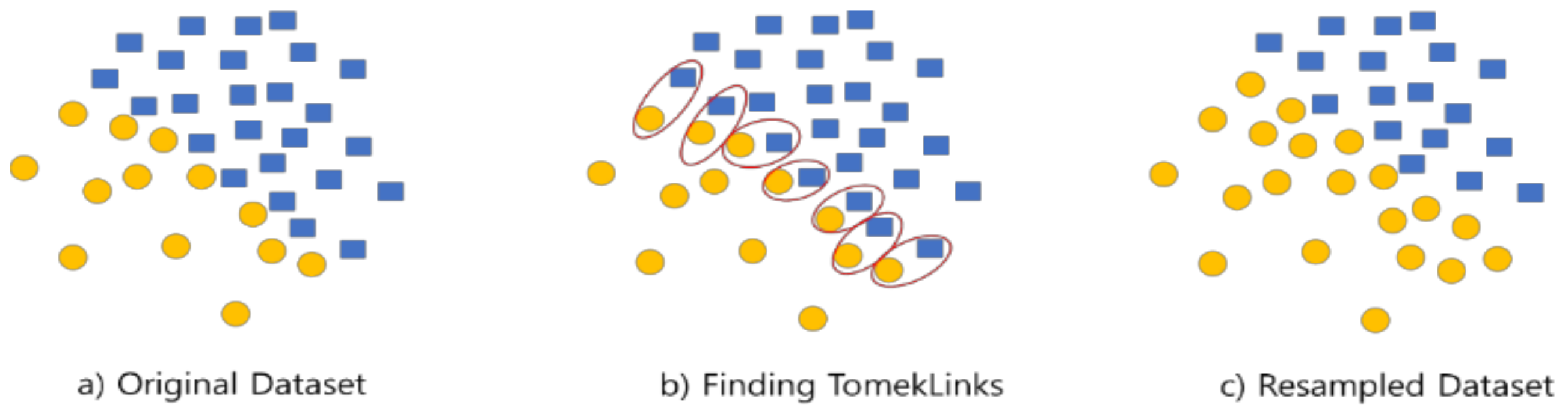
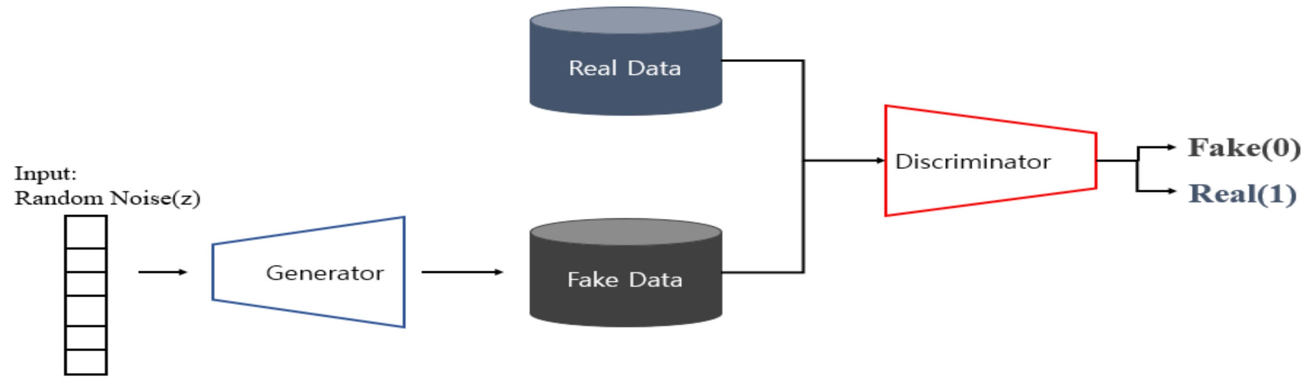
4.1.4. Data Imbalance Handling

As the last step of preprocessing, we used six methods in order to resolve the data imbalance problem. These were random oversampling for the minority class, SMOTE, SMOTE-Tomek, SMOTE-ENN, and ADASYN, which oversamples the minority class and undersamples the majority class, and GAN, which generates balanced data by synthesizing virtual data after learning the data of the insufficient class based on the actual data distribution.

4.2. Building the Classifcation Model and Evaluation

Forty-two datasets were created by applying six methodologies to resolve data imbalances in seven datasets that required replacement of missing values. By comparing the quality classification performance of the datasets, we tried to find the combination that showed the best performance.

In order to prevent the overfitting of training data and testing data, we tried to achieve optimal performance by the model by using the time series cross validation method, which is one of the cross validation methods. In the existing cross validation method, because training, testing, and verification are performed regardless of the time flow, the performance of the current model may be high, but the performance cannot be guaranteed when future data are learned. Therefore, in using time series cross validation, the time flow is divided into regular intervals, and the verification interval is tuned so that it can be evaluated using future data rather than the training interval.

In machine learning and deep learning, parameters are variables that can be checked inside the model and then become values that can be calculated through data. They also play an important role when learning a methodology, as they determine the performance of the model. In the “building a classification model” stage, logistic regression, KNN, random forest, decision tree, and SVC methodologies were used to classify the quality of the semiconductor manufacturing process. In order for these methodologies to find the optimal parameter settings and show higher performance for model training, a hyperparameter search and model optimization were performed.

Finally, the model performance was calculated based on the F1 score. When the data class has an imbalanced structure, the performance of the model can be accurately evaluated using the F1 score. The F1 score is the harmonic average of Precision and Recall, as shown below. Precision means the proportion of those whose original value is True among those classified as True by the classification model, and Recall means the ratio of what the classification model predicts as True among those that are actually True. Precision is a measure of result relevancy, while Recall is a measure of how many truly relevant results are returned.

$$\mathrm{F}1=2\times \frac{1}{\frac{1}{Precision}+\frac{1}{Recall}}=2\times \frac{Precision\times Recall}{Precision+Recall}$$

An analysis of variance (ANOVA) was performed to identify significant results in the cases where missing data, imbalances, and hyperparameters were applied differently for the five methods except for the GAN.

5. Experimental Setting and Results

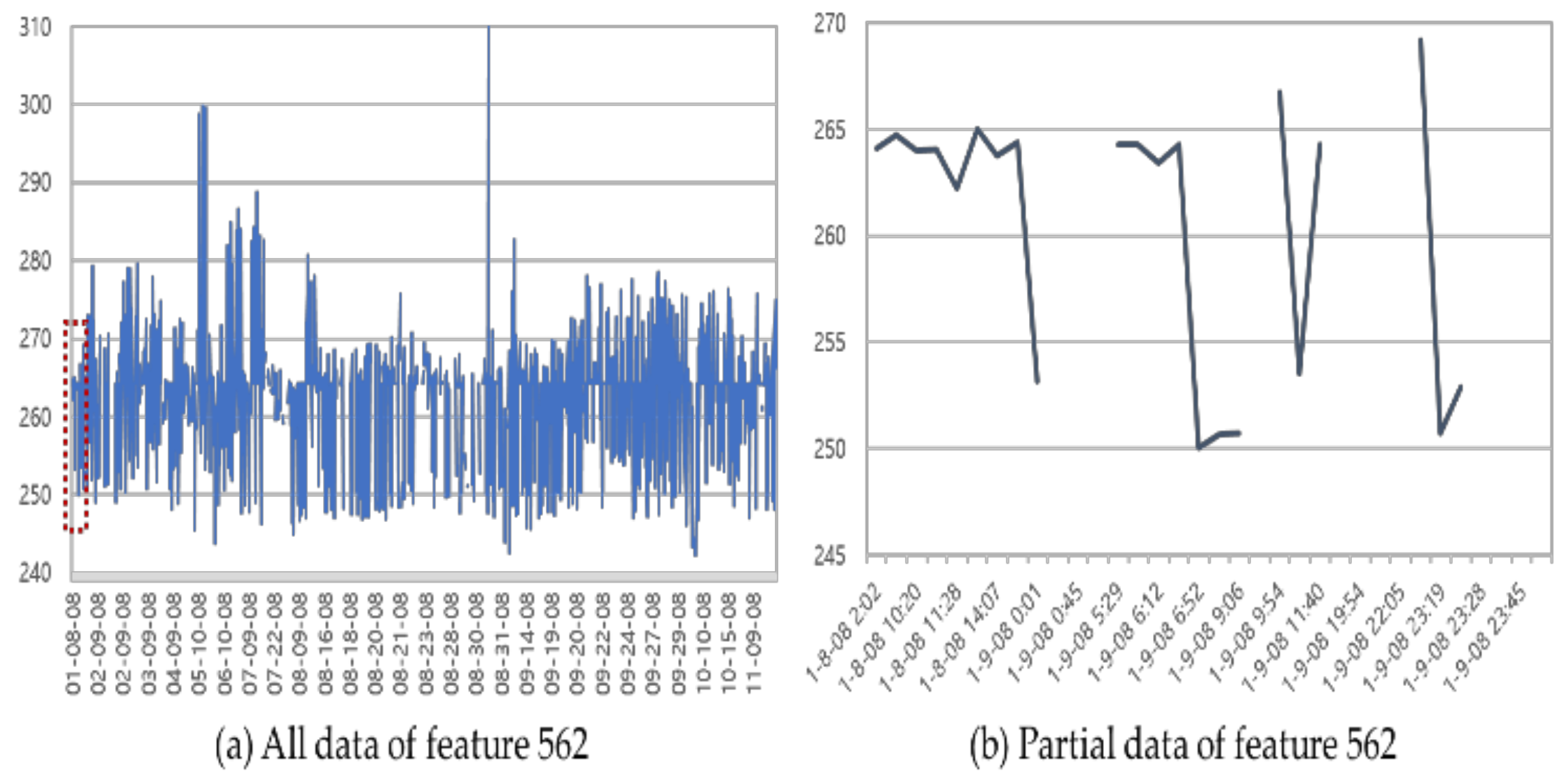
5.1. Dataset

Among the 1567 total data observations in the SECOM dataset, 1463 (93.36%) had good quality (Pass) and 104 (6.64%) had bad quality (Fail). The number of independent variables in the data was 436, excluding the variables that had a large proportion of missing values or that contained single values, and a binary variable representing a good or bad status was used as a dependent variable. Additionally, some variables included missing values, as in the example shown in Figure 4.

5.2. Experimental Settings

Because the dataset contains a large number of features, the number of significant features (from 5 to 40) was calculated to improve the performance of all methodologies.

In the case of logistic regression, the optimal performance of the model was calculated by specifying the range of cost function values and the range of the solver that determines the algorithm to be used for optimization.

In the case of KNN, the values of the metric k and the weight, which are methods for measuring distance, are specified. The classification of new data varies depending on how the distance is measured and how the standard is set. Additionally, if the value of k is too small, the optimal conditions for the parameters are searched for because there is a risk of overfitting, which yields high accuracy in the training process but low accuracy in the testing process.

In the case of SVC, the parameter values of C, gamma, and kernel were specified. Depending on the value of C, overfitting can be prevented. The larger the gamma, the more accurate the model, and the smaller the gamma, the more overfitting can be prevented. By specifying the value of the kernel, we want to achieve optimal learning by changing the data to a higher level and discarding the necessary properties. In the case of the random forest and decision tree methodologies, we tried to find the optimal methodology by designating max_features considering the ratio of referencing data variables, min_samples_split considering the minimum amount of data for splitting nodes, and the classification criterion.

Table 5. Python libraries used for the analysis.

Package	Version	Description
numpy	1.18.1	Provides useful functions for scientific calculations, especially for handling multidimensional arrays
pandas	0.25.3	Widely used for data analysis
scikit-learn	0.23.0	Machine learning library
imbalanced-learn	0.7.0	Implements various sampling methods to solve the imbalanced data problem
mlxtend	0.17.3	Composed of useful tools for common data science tasks
tqdm	4.42.1	Creates a progress bar on the fly and predicts the Time to Completion (TTC) of a function or loop
keras	2.2.4	Makes it easy to handle deep learning engines such as TensorFlow with python

shows the hyperparameters of each model used in this study. In addition, the level and setting values for each factor are also summarized in this table. The factors and levels were set and analyzed in order to determine the significance between data pre-processing combinations. The values of the factor for the imputation methodologies were assigned serial numbers by the experimental methodology, so the values of KNN (k = 2): 1, KNN (k = 4): 2, KNN (k = 6): 3, LI: 4, MICE: 5, MissForest: 6, and PI: 7 were set. The methodologies related to the handling of imbalances were also set as ADASYN: 1, SMOTE: 2, Random Oversampling: 3, SMOTE-Tomek: 4, and SMOTE-ENN: 5. After the classification model was analyzed, factor analysis was performed using the parameter values for the top 10 F1 scores on each dataset.

As the parameters for the GAN experiment, the learning rate was set to 0.00001, the momentum coefficient (beta) was 0.8, the activation function of the generator and the discriminator was a rectified linear unit (ReLU) function with a coefficient of 0.2, and the batch size was set to 32. The seven datasets generated by replacing missing data were set to run 10,000 times. The Python version used for analysis was version 3.6.12, Jupyter was used as the integrated development environment, and the libraries used are shown in

Table 6. Model parameters and setting ranges for each methodology.

Method	Hyperparameter	Range	Level	Setting Value
Logistic Regression	C	[0.0001, 0.001, 0.01, 1, 10, 100, 1000]	7
	solver	[liblinear, newton-cg]	2	1,2
	Feature		7	5,10,15,20,25,30,35
KNN	metric	[manhattan, euclidean, minkowski]	3	1,2,3
	weights	[uniform, distance]	2	1,2
	n_neighbors	1 <= k <= 21	3	1,2,3
	Feature		5	15,20,25,30,35
SVC	C	[0.001, 0.01, 0.1, 1]	4
	gamma	[0.01, 0.1, 1]	3
	kernel	[poly, rbf, linear]	3	1,2,3
	Feature		5	15,20,25,30,35
Decision Tree	max_features	[auto, sqrt, log2]	3	1,2,3
	min_samples_split	3 <= n <= 10	8	3,4,5,6,7,8,9,10
	max_depth	1 <= n <= 10	9	1,3,4,5,6,7,8,9,10
	criterion	[gini, entropy]	2	1,2
	Feature		7	5,10,15,20,25,30,35
Random Forest	max_features	[auto, sqrt, log2]	3	1,2,3
	min_samples_split	3 <= n <= 10	6	3,4,5,6,7,8
	criterion	[gini, entropy]	2	1,2
	Feature		6	5,10, 20,25,30,35

.

5.3. Results

5.3.1. Performance Evaluation of Classification Models

Table 7. Quality classification.

		Random Oversampling	SMOTE	SMOTE-Tomek	SMOTE- ENN	ADASYN	GAN
Linear Interpolation		0.292	0.532	0.534	0.815	0.517	0.898
Poly Interpolation		0.293	0.535	0.529	0.818	0.531	0.899
KNN (k = 2)		0.302	0.540	0.537	0.818	0.531	0.904
KNN (k = 4)		0.301	0.535	0.538	0.814	0.530	0.912
KNN (k = 6)		0.301	0.534	0.538	0.814	0.535	0.915
MICE		0.301	0.542	0.536	0.795	0.529	0.907
MissForest		0.301	0.540	0.538	0.817	0.519	0.889

shows the performance of the model that classified quality by imputation and imbalance handling. When missing values were replaced using the KNN method with k = 6 and data imbalance processing used the GAN, the F1 score was the highest at 0.915. It can be seen that the method proposed in this study has a higher F1 score than the score of 0.192 by [8] and the score of 0.356 by [5], which are the results of studies conducted with the same dataset. The GAN is a deep neural network composed of two networks, a generator, and a discriminator. In this method, because the current network and other networks compete and learn, it is possible to learn to imitate the distribution of the data, which seems to provide better performance than the existing methods for resolving data imbalances.

5.3.2. Evaluation of Combinations of Classification Models for Data Preprocessing

As manufacturing processes undergo innovation, and a variety of data are collected, the data imbalance problem will tend to increase. In order to solve this problem, the quality classification performance can be improved using the GAN, but the GAN has disadvantages in that it takes a long time to learn and requires a considerable amount of computing power.

To supplement this, we propose a technique for finding the optimal data preprocessing combination by identifying the significance between parameters in the methodologies frequently used for classification.

For each methodology, to determine whether there is a significant difference in F1 scores between missing values, imbalances, and hyperparameters, the null hypothesis was set as the absence of a difference, and then an ANOVA was performed. If the p-value is smaller than the significance level, the null hypothesis can be rejected and the missing value, imbalance, and hyperparameter can be judged to have significance. In this study, the significance level was set to 0.05, and the results are shown in

Table 8. Result of ANOVA for F1 scores for each method and its factors.

Method	Source		Degrees of Freedom	AdjSS	AdjMS	F-Value	p-Value
KNN	Factors	Missing	6	0.001	0.000	9.440	0.000
		Imbalance	4	5.175	1.294	56,839.100	0.000
		metric	2	0.000	0.000	2.530	0.081
		n_neighbors	2	0.001	0.000	13.580	0.000
		weights	1	0.000	0.000	1.850	0.175
		Number of Features	4	0.002	0.001	23.060	0.000
	Error		330	0.008	0.000
SVC	Factors	Missing	6	0.007	0.001	4.450	0.000
		Imbalance	4	9.766	2.442	9539.580	0.000
		C	3	0.019	0.006	24.160	0.000
		gamma	2	0.002	0.001	4.740	0.009
		kernel	1	0.000	0.000	1.330	0.249
		Number of Features	4	0.024	0.006	23.880	0.000
	Error		329	0.084	0.000
Decision Tree	Factors	Missing	6	0.006	0.001	19.800	0.000
		Imbalance	4	3.458	0.864	16,731.730	0.000
		criterion	1	0.000	0.000	2.490	0.116
		max_depth	8	0.002	0.000	5.960	0.000
		max_features	2	0.000	0.000	0.430	0.653
		min_sample_split	7	0.001	0.000	1.740	0.099
		Number of Features	6	0.001	0.000	2.730	0.013
	Error		315	0.016	0.000
Random Forest	Factors	Missing	6	0.026	0.004	88.110	0.000
		Imbalance	4	7.185	1.796	37,046.710	0.000
		criterion	1	0.000	0.000	0.000	0.960
		max_depth	2	0.000	0.000	1.830	0.162
		min_sample_split	5	0.001	0.000	3.650	0.003
		Number of Features	5	0.002	0.000	6.160	0.000
	Error		326	0.016	0.000
Logistic Regression	Factors	Missing	6	0.002	0.000	1.710	0.118
		Imbalance	4	15.107	3.777	25,898.740	0.000
		C	5	0.078	0.016	107.180	0.000
		solver	1	0.001	0.001	4.440	0.036
		Number of Features	6	0.039	0.006	43.980	0.000
	Error		327	0.048	0.000

.

For the evaluation index, which was the F1 score, the Missing, Imbalance, and Number of Features factors were found to be significant for most methodologies. Among the factors showing significant results, the n_neighbors (k) of KNN, the C and gamma of SVC, and the C of logistic regression are related to the prevention of overfitting. In the case of the decision tree methodology, max_depth seems to have a significant effect by adjusting parameters by setting the learning depth in advance to increase the generalization performance. In the case of the random forest methodology, min_sample_split can be seen to affect the F1 score by controlling overfitting and by stopping learning at nodes less than the corresponding number, as in the decision tree methodology. In the case of logistic regression, it was found that the solver that determines the algorithm to be used for optimization has a significant effect on the F1 score.

In addition, the calculation results for the main effects for each parameter by methodology are shown in Figure 5. The purpose of this analysis is to determine the significance of data preprocessing among the results of the 35 datasets generated after replacing missing values, except for the GAN, and resolving imbalances. For the 35 datasets, the missing values, imbalances, and parameter combinations were analyzed for the top 10 F1 scores obtained using the KNN methodology. The figures illustrate the main effects for the F1 score.

The results of the main effects analysis show that in the case of imputation, the effect of each level is similar for all methodologies, and the application of SMOTE-ENN shows the greatest effect for imbalance handling. In KNN, the “Euclidean” distance has the highest effect on the metric, and the optimal Number of Features shows a tendency to increase the influence on the F1 score as the value of k increases. In the case of SVC, as the parameter values of C and gamma increase, the effect on the F1 score decreases. As for the number of features, the influence on the F1 score tends to increase somewhat as the value of k increases. For the decision tree methodology, learning is stopped at nodes less than the corresponding number, and it can be seen that the effect is large when min_sample_split is 9. The optimal number of features shows a large influence on the F1 score when the number of variables is 20. The criterion for the random forest methodology is related to the criterion that calculates the information gain used to separate the branches, and when the value is “entropy”, the effect on the F1 score is large. For logistic regression, when C is 0.01 and the solver is “newton-cg”, the effect on the F1 score is large.

6. Conclusions and Future Research

With the large amount of interest in smart manufacturing, at a manufacturing site, missing values occur during data collection due to sensor failures or machine failures or for unknown reasons. Finally, data classes become unevenly distributed, which causes a data imbalance. To solve this problem, machine learning and deep learning could be used to obtain meaningful information about the process state from the data on the manufacturing process, and these methods are often used to explore important variables for quality improvement or information to be used to judge quality. However, machine learning and deep learning methods still have limitations when the data are missing or imbalanced.

In this study, considering the case in which data cannot be collected, i.e., there are missing data, we created a number of datasets by replacing missing values in the data using various methods, and we applied methods that have been widely used to solve data imbalance problems, including the GAN, which has been widely studied recently, and finally we used combinations that increased the performance of the methodologies. When missing values were replaced using the KNN methodology, and the GAN was applied to the imbalance problem, the F1 score was 0.915, which is much higher than the 0.356 obtained in a previous study by [5]. Because the GAN has shortcomings, such as a long learning time and high computing power requirements, to compensate for this, we investigated a data preprocessing combination of the methodologies most used in existing classification studies, and then we measured the significance of each factor to the F1 score. In the case of imputation, all methodologies except for logistic regression had an effect on the F1 score, and in the case of data imbalance handling, it was confirmed that there was an effect for all methodologies.

This study proposed a procedural framework that can be applied to other datasets. It has been shown that meaningful parameters can be identified during data preprocessing using the open dataset provided by UCI. Although it was difficult to understand exactly what each data observation meant and to interpret the results due to the limitations of the open dataset, it will be possible to increase the efficiency of the analysis by applying the framework to other datasets of manufacturing processes in the future.

References

1. Kim, H.; Lee, H. Fault Detect and Classification Framework for Semiconductor Manufacturing Processes using Missing Data Estimation and Generative Adversary Network. J. Korean Inst. Intell. Syst. 2018, 28, 393–400. [Google Scholar]
2. Randolph-Gips, M. A new neural network to process missing data without Imputation. In Proceedings of the 2008 Seventh International Conference on Machine Learning and Applications, San Diego, CA, USA, 11–13 December 2008; pp. 756–762. [Google Scholar]
3. O’Brien, R.; Ishwaran, H. A random forests quantile classifier for class imbalanced data. Pattern Recognit. 2019, 90, 232–249. [Google Scholar] [CrossRef] [PubMed]
4. Napierała, K.; Stefanowski, J. Addressing imbalanced data with argument based rule learning. Expert Syst. Appl. 2015, 42, 9468–9481. [Google Scholar] [CrossRef]
5. Munirathinam, S.; Ramadoss, B. Predictive models for equipment fault detection in the semiconductor manufacturing process. IACSIT Int. J. Eng. Technol. 2016, 8, 273–285. [Google Scholar] [CrossRef] [Green Version]
6. Moldovan, D.; Cioara, T.; Anghel, I.; Salomie, I. Machine learning for sensor-based manufacturing processes. In Proceedings of the 2017 13th IEEE International Conference on Intelligent Computer Communication and Processing (ICCP), Cluj-Napoca, Romania, 7–9 September 2017; pp. 147–154. [Google Scholar]
7. Chomboon, K.; Kerdprasop, K.; Kerdprasop, N. Rare class discovery techniques for highly imbalance data. In Proceedings of the International MultiConference of Engineers and Computer Scientists, Hong Kong, China, 13–15 March 2013; Volume 1. [Google Scholar]
8. Kerdprasop, K.; Kerdprasop, N. Feature selection and boosting techniques to improve fault detection accuracy in the semiconductor manufacturing process. In Proceedings of the International MultiConference of Engineering and Computer Scientists 2011 (IMECS 2011), Hong Kong, China, 16–18 March 2011; Volume 1. [Google Scholar]
9. Kim, J.; Han, Y.; Lee, J. Data imbalance problem solving for smote based oversampling: Study on fault detection prediction model in semiconductor manufacturing process. Adv. Sci. Technol. Lett. 2016, 133, 79–84. [Google Scholar]
10. García-Laencina, P.J.; Sancho-Gómez, J.L.; Figueiras-Vidal, A.R.; Verleysen, M. K nearest neighbours with mutual information for simultaneous classification and missing data imputation. Neurocomputing 2009, 72, 1483–1493. [Google Scholar] [CrossRef]
11. Stekhoven, D.J.; Bühlmann, P. MissForest—Non-parametric missing value imputation for mixed-type data. Bioinformatics 2012, 28, 112–118. [Google Scholar] [CrossRef] [PubMed] [Green Version]
12. Schmitt, P.; Mandel, J.; Guedj, M. A comparison of six methods for missing data imputation. J. Biom. Biostat. 2015, 6, 1. [Google Scholar]
13. García-Laencina, P.J.; Abreu, P.H.; Abreu, M.H.; Afonoso, N. Missing data imputation on the 5-year survival prediction of breast cancer patients with unknown discrete values. Comput. Biol. Med. 2015, 59, 125–133. [Google Scholar] [CrossRef] [PubMed]
14. Bauer, J.; Angelini, O.; Denev, A. Imputation of multivariate time series data-performance benchmarks for multiple imputation and spectral techniques. SSRN Electron. J. 2017. [Google Scholar] [CrossRef]
15. Van Hulse, J.; Khoshgoftaar, T.M.; Napolitano, A. Experimental perspectives on learning from imbalanced data. In Proceedings of the 24th International Conference on Machine Learning, Corvallis, OR, USA, 20–24 June 2007; pp. 935–942. [Google Scholar]
16. Son, M.; Jung, S.; Hwang, E. Oversampling scheme using Conditional GAN. In Proceedings of the Korea Information Processing Society Conference, Pusan, Korea; Korea Information Processing Society, 2018; pp. 609–612. [Google Scholar]
17. Lamari, M.; Azizi, N.; Hammami, N.E.; Boukhamla, A.; Cheriguene, S.; Dendani, N.; Benzebouchi, N.E. SMOTE–ENN-Based Data Sampling and Improved Dynamic Ensemble Selection for Imbalanced Medical Data Classification. In Advances on Smart and Soft Computing; Springer: Singapore, 2020; pp. 37–49. [Google Scholar]
18. Chawla, N.V.; Bowyer, K.W.; Hall, L.O.; Kegelmeyer, W.P. SMOTE: Synthetic minority over-sampling technique. J. Artif. Intell. Res. 2002, 16, 321–357. [Google Scholar] [CrossRef]
19. Batista, G.E.; Prati, R.C.; Monard, M.C. A study of the behavior of several methods for balancing machine learning training data. ACM SIGKDD Explor. Newsl. 2004, 6, 20–29. [Google Scholar] [CrossRef]
20. Liang, G. An effective method for imbalanced time series classification: Hybrid sampling. In Australasian Joint Conference on Artificial Intelligence; Springer: Cham, Switzerland, 2013; pp. 374–385. [Google Scholar]
21. Branco, P.; Torgo, L.; Ribeiro, R. A survey of predictive modelling under imbalanced distributions. arXiv 2015, arXiv:1505.01658. [Google Scholar]
22. He, H.; Bai, Y.; Garcia, E.A.; Li, S. ADASYN: Adaptive synthetic sampling approach for imbalanced learning. In Proceedings of the 2008 IEEE International Joint Conference on Neural Networks (IEEE World Congress on Computational Intelligence), Hong Kong, China, 1–6 June 2008; pp. 1322–1328. [Google Scholar]
23. Boser, B.E.; Guyon, I.M.; Vapnik, V.N. A training algorithm for optimal margin classifiers. In Proceedings of the Fifth Annual Workshop on Computational Learning Theory, Pittsburgh, PA, USA, 27–29 July 1992; pp. 144–152. [Google Scholar]
Figure 1. Creation of TomekLinks.
Electronics 11 00477 g001
Figure 2. GAN framework.
Electronics 11 00477 g002
Figure 3. Framework for imputation and imbalance adjustment.
Electronics 11 00477 g003
Figure 4. Example of identifying a missing value in the data of feature 562.
Electronics 11 00477 g004
Figure 5. F1 scores for each of the methodologies.
Electronics 11 00477 g005