
Real-Time 3D Object Detection and Classification in Autonomous Driving Environment Using 3D LiDAR and Camera Sensors
 , and
, and
Abstract
:1. Introduction
- In OD-C3DL, the Point Cloud Augmentation (PCA) process estimates the depth information from the camera sensor data and coordinates the spatial information of the object, which enhances object identification to a greater extent.
- The PCA process specifically uses the pre-trained Pyramid Stereo Matching Network (PSMNet), which exploits the global contextual information and extends the pixel-level features to region-level features with different scales of receptive fields to compute the disparity map.
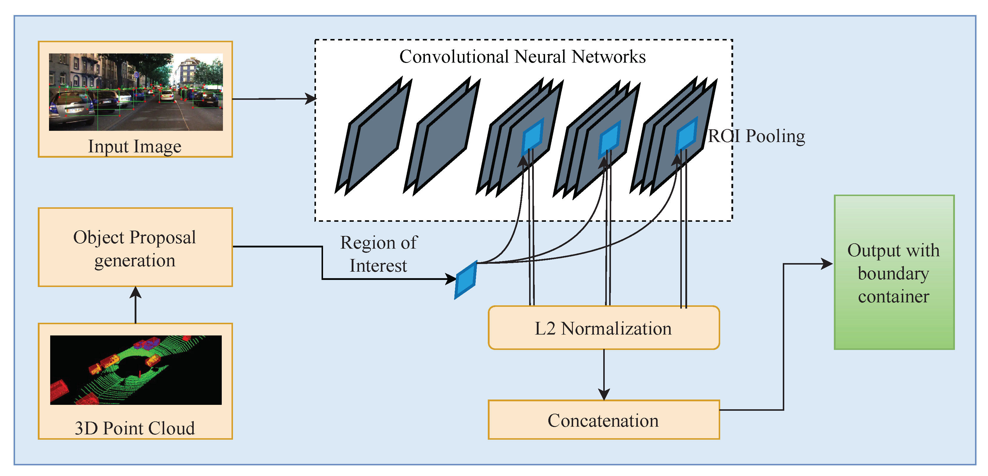
- The OD-C3DL applies VGG16 to implement ROI pooling next to the convolutional layers such as Conv3, Conv4, and Conv5, rather than just on the final convolutional layer, in which a feature tensor of fixed size is produced by each layer.
- The OD-C3DL standardizes the attribute tensor utilizing L2 standardization and concatenates all the standardized attribute tensors, which ensures the detection system’s reliability and scales the attribute associations arising out of several convolution layers to the equivalent size.
- The OD-C3DL encompasses multiple task loss such as boundary container regression loss and classification loss functions for accomplishing object classification and boundary container regression at the training stage.
2. Related Work
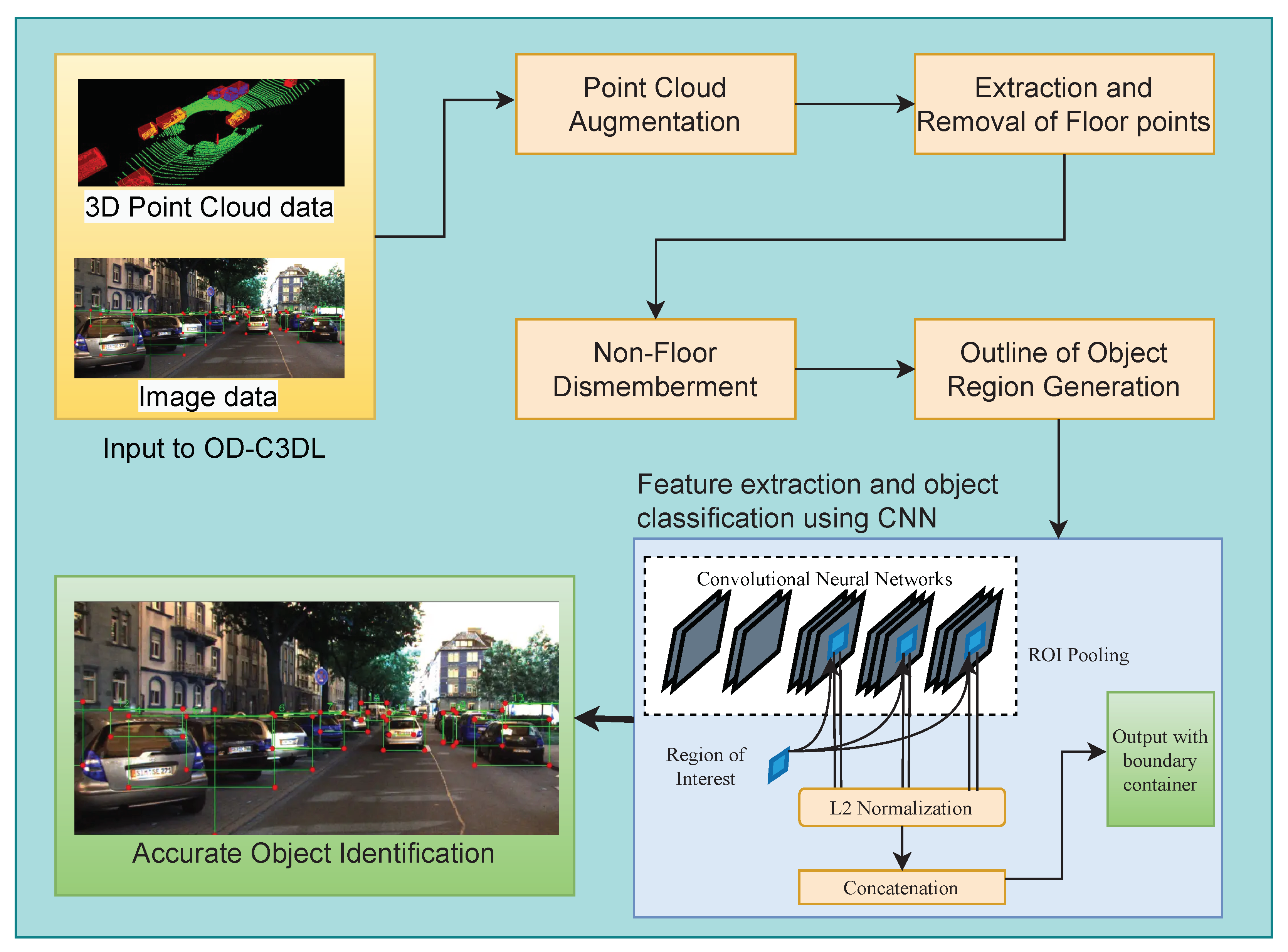
3. Proposed Work
- Augmentation of point clouds
- Object region identification
- Feature extraction and object classification using CNN
3.1. Point Cloud Augmentation
3.2. Object Region Identification (ORI) with 3D LiDAR Data
- Extraction and removal of floor points
- Non-floor dismemberment
- Outline of object region generation
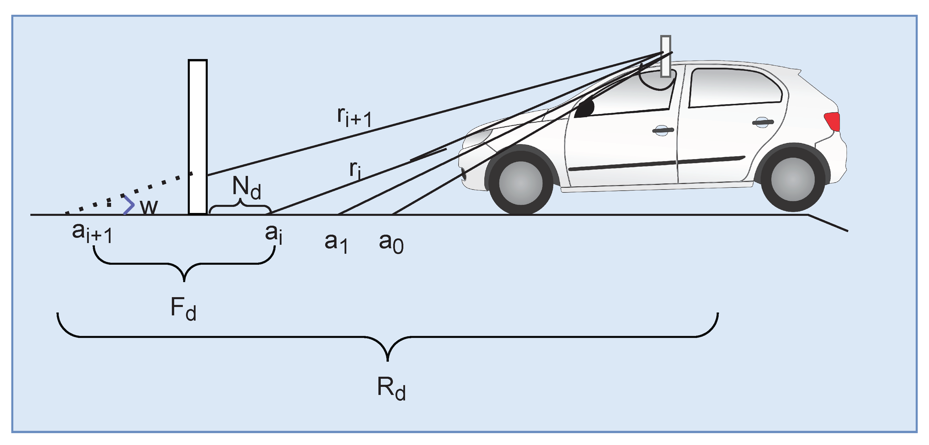
3.2.1. Extraction and Removal of Floor Points
3.2.2. Non-Floor Dismemberment
| Algorithm 1 Cluster-based non-floor point dismemberment Algorithm. |
Input: Non-floor points () floor partitioning methodology, azimuth limit difference () Output: Decisive set of cluster non-floor points (R)
|
3.3. Feature Extraction and Object Classification Using CNN
4. Evaluation of the Proposed Work
4.1. Performance Analysis of Proposed Methodology
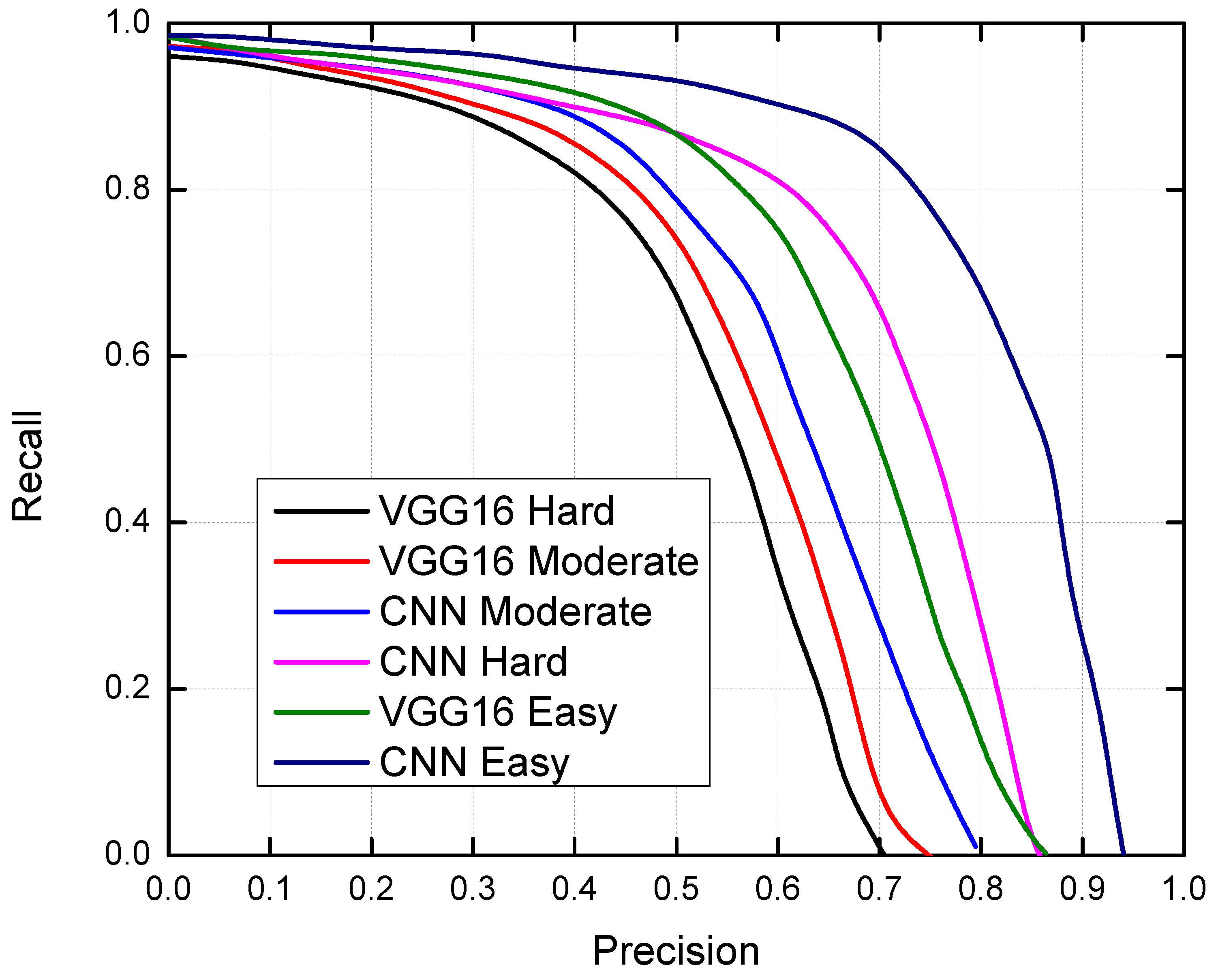
4.1.1. Analysis of Precision Recall Curve
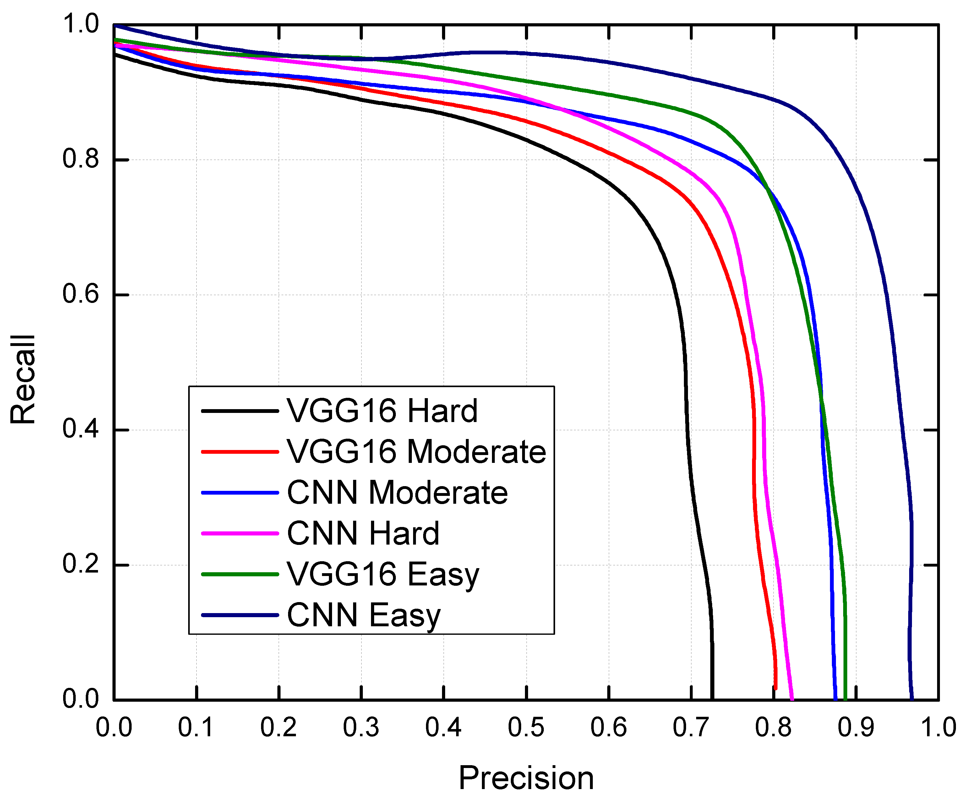
4.1.2. Analysis of Accuracy Gains
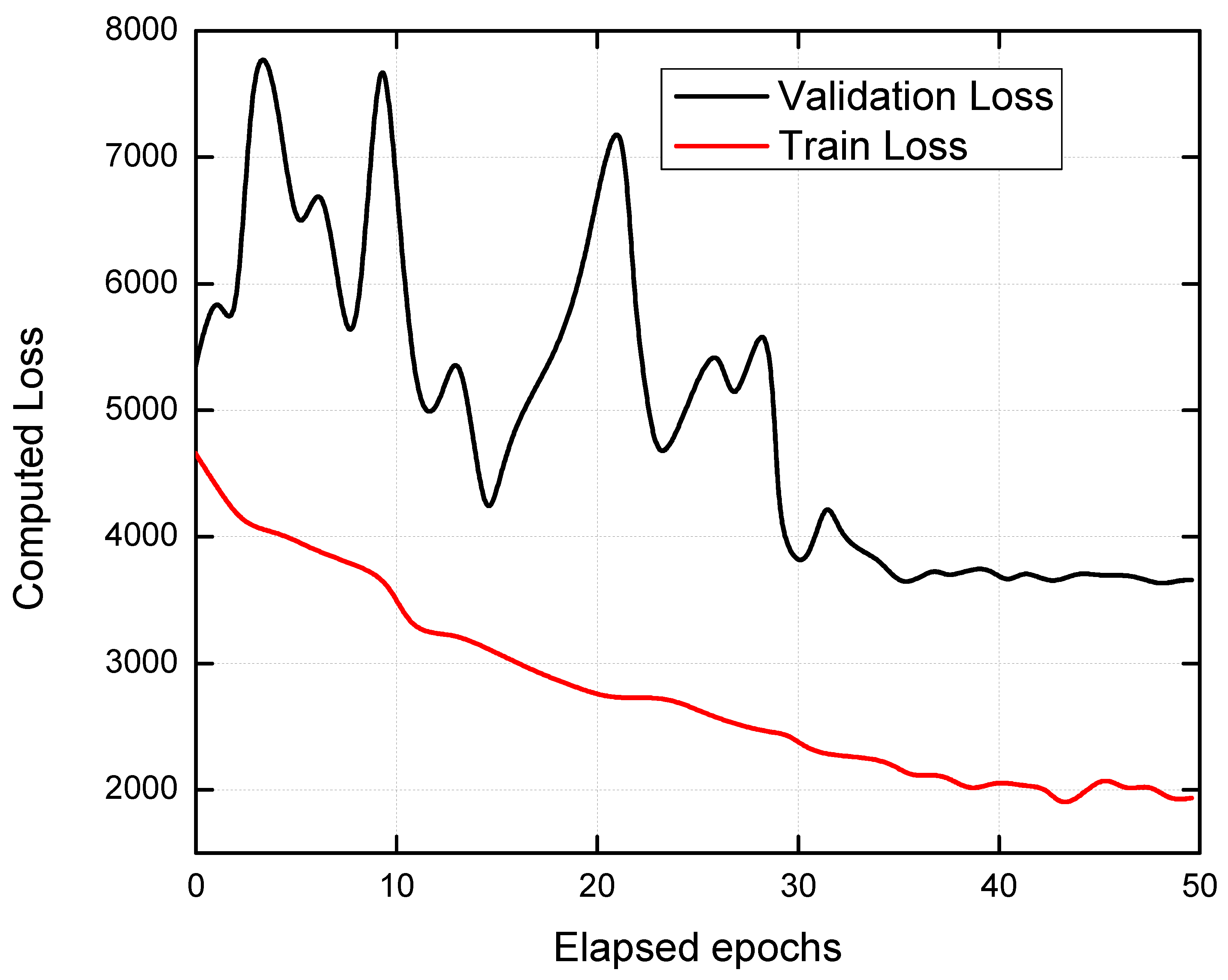
4.1.3. Analysis of Elapsed Epochs vs. Computed Loss for the CNN Model
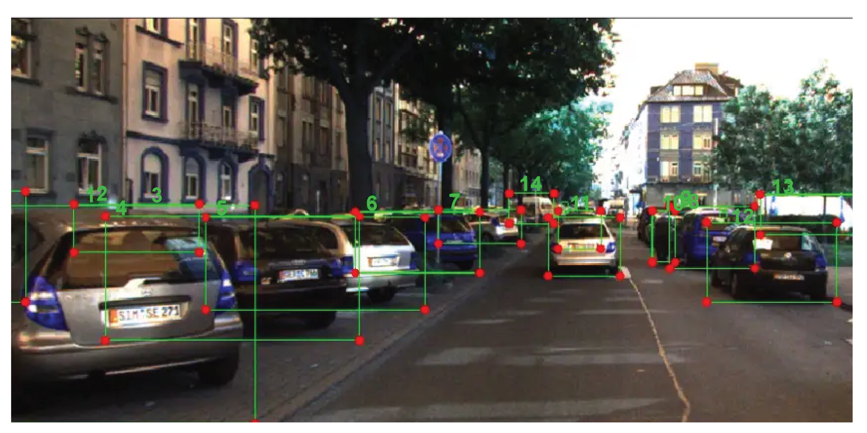
4.1.4. Analysis of Object Detection under Various States
4.2. Comparative Analysis of Proposed Methodology
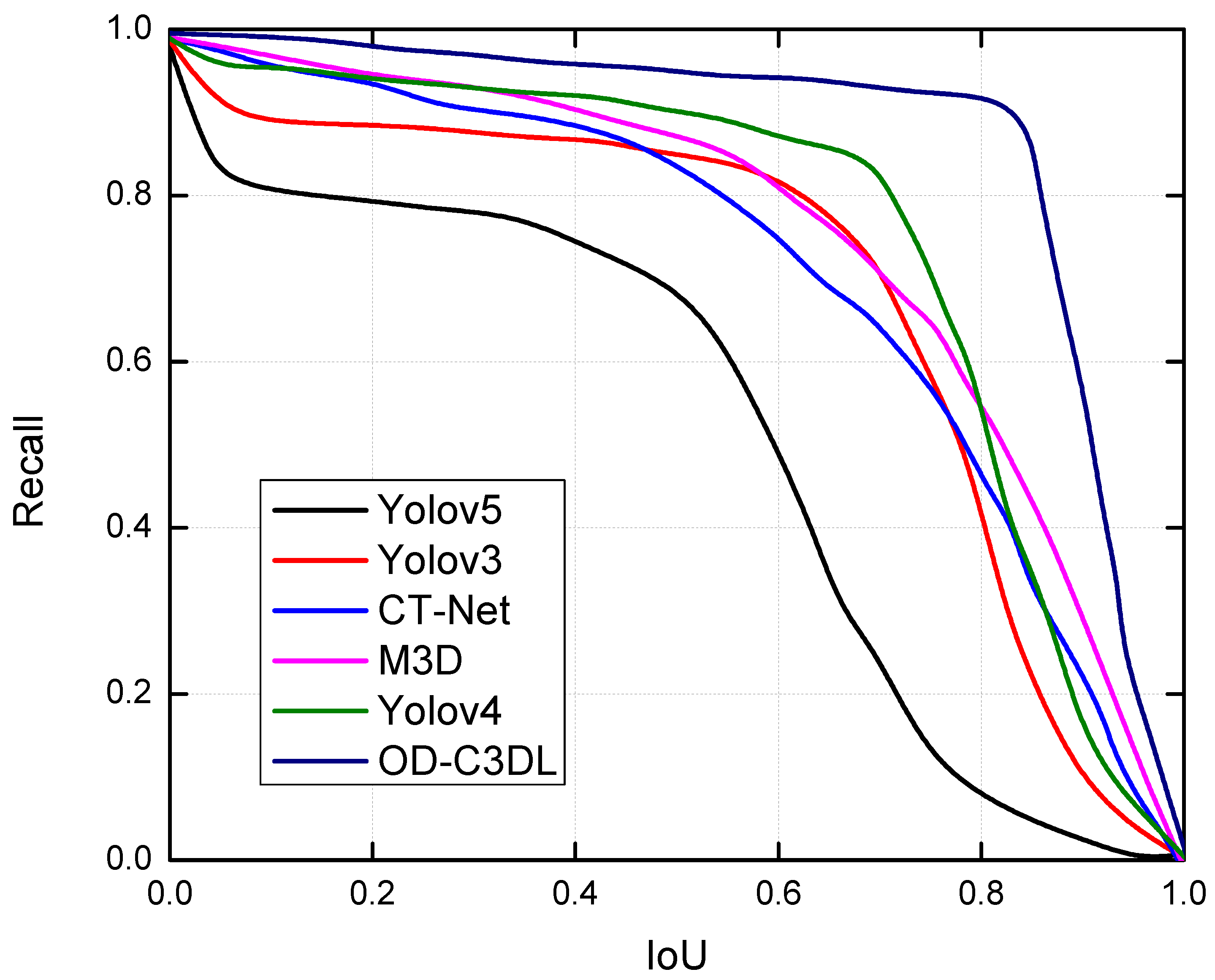
4.2.1. Comparative Analysis of Recall vs. IoU
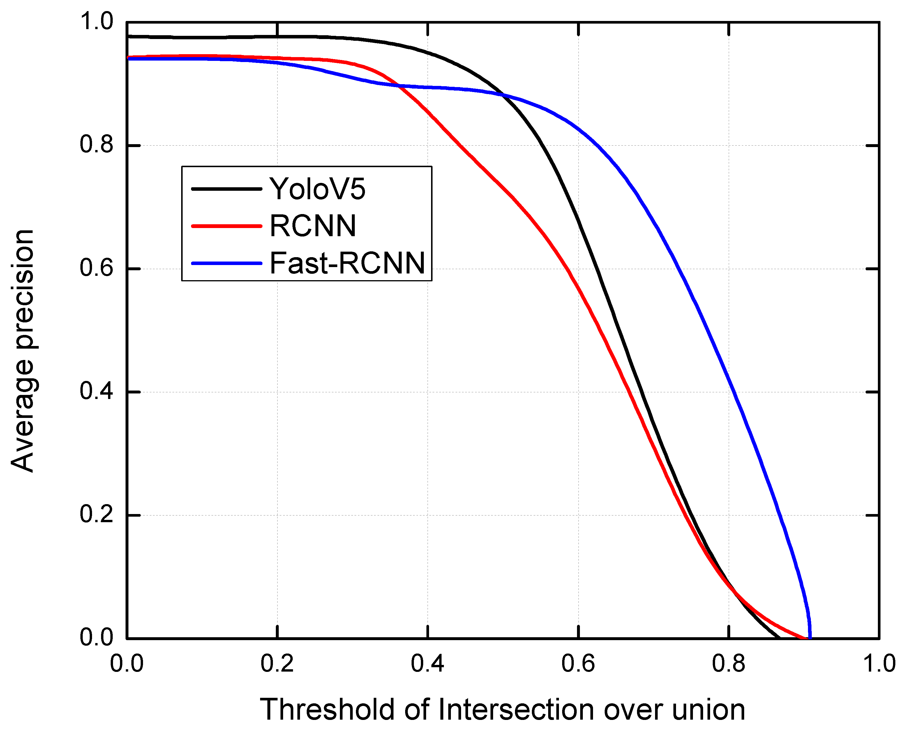
4.2.2. Comparative Analysis of Average-Precision
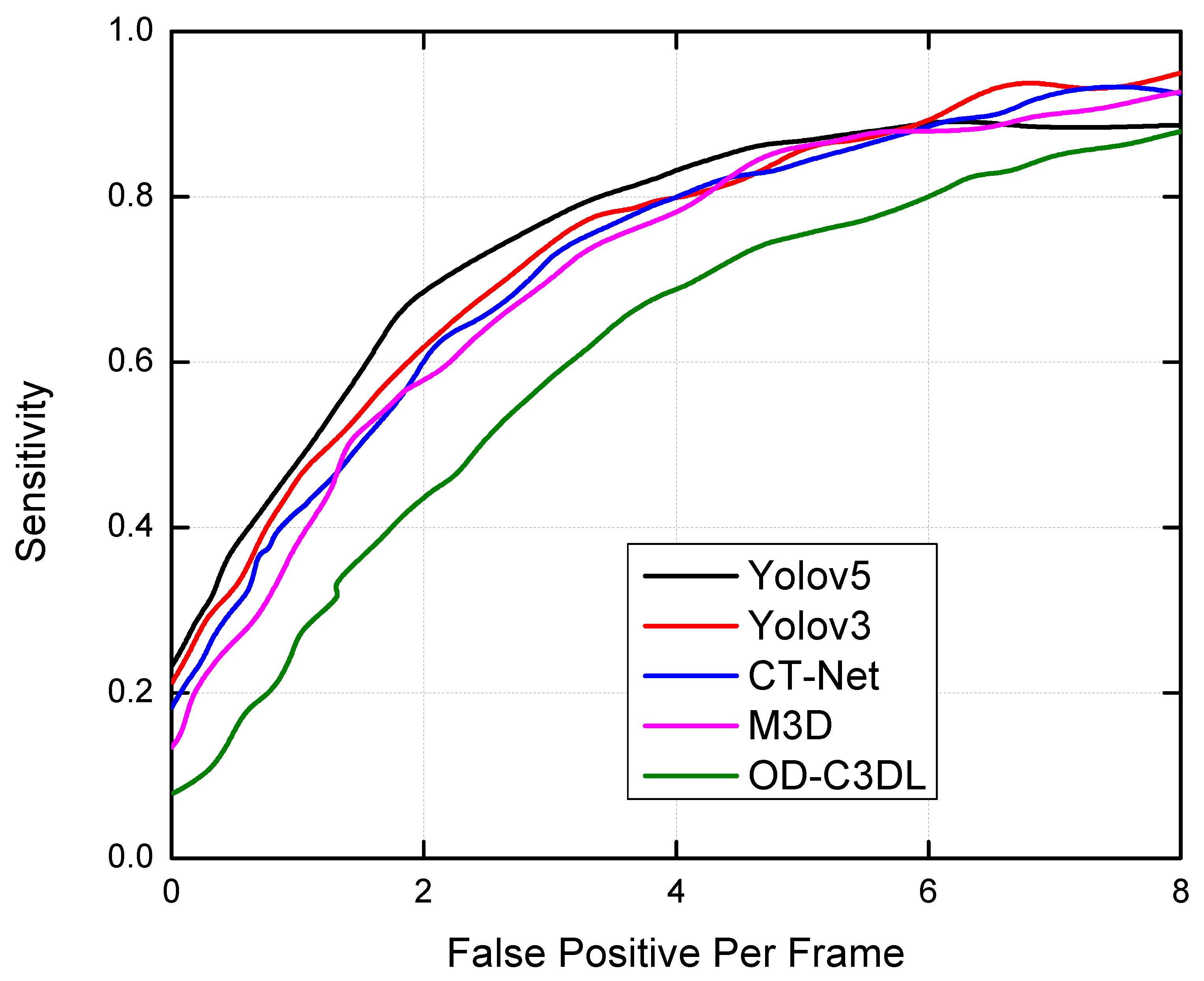
4.2.3. Comparative Analysis of Sensitivity and Average Precision
5. Conclusions
Author Contributions
Funding
Data Availability Statement
Conflicts of Interest
Abbreviations
| AVs | Autonomous Vehicles |
| LiDAR | Light Detection and Ranging |
| 3D LiDAR | Three-Dimensional Light Detection and Ranging |
| ROI | Regions of Interest |
| IoU | Intersection over Union |
| CNN | Convolutional Neural Networks |
| V2I | Vehicle-to-Infrastructure |
| HMM | Hidden Markov model |
| RSSI | Received signal strength indicator |
| CT-Net | Convolution Transformer Network |
| FGPA | Field Programmable Gate Array |
| M3D | Monocular camera is used to detect the 3D object |
| PCA | Point Cloud Augmentation |
| PSMNet | Pyramid Stereo Matching Network |
| ORI | Object Region Identification |
| NFD | Non-Floor Dismemberment |
| NAG | Nesterian Accelerated Gradient |
| Fast-RCNN | Fast-Regions with CNN |
| AP | Average-Precision |
| PNN | Probabilistic Neural Network |
References
- Lee, S.; Lee, D.; Choi, P.; Park, D. Accuracy–power controllable LiDAR sensor system with 3D object recognition for autonomous vehicle. Sensors 2020, 20, 5706. [Google Scholar] [CrossRef] [PubMed]
- Francies, M.L.; Ata, M.M.; Mohamed, M.A. A robust multiclass 3D object recognition based on modern YOLO deep learning algorithms. Concurr. Comput. Pract. Exp. 2022, 34, e6517. [Google Scholar] [CrossRef]
- Gupta, B.B.; Gaurav, A.; Marín, E.C.; Alhalabi, W. Novel Graph-Based Machine Learning Technique to Secure Smart Vehicles in Intelligent Transportation Systems. IEEE Trans. Intell. Transp. Syst. 2022, 1–9. [Google Scholar] [CrossRef]
- Prathiba, S.B.; Raja, G.; Anbalagan, S.; Dev, K.; Gurumoorthy, S.; Sankaran, A.P. Federated Learning Empowered Computation Offloading and Resource Management in 6G-V2X. IEEE Trans. Netw. Sci. Eng. 2022, 9, 3234–3243. [Google Scholar] [CrossRef]
- Zhang, X.; Xia, X.; Liu, S.; Cao, Y.; Li, J.; Guo, W. An Integrated Framework on Autonomous-EV Charging and Autonomous Valet Parking (AVP) Management System. IEEE Trans. Transp. Electrif. 2022, 8, 2836–2852. [Google Scholar] [CrossRef]
- Deb, S.; Carruth, D.W.; Hudson, C.R. How communicating features can help pedestrian safety in the presence of self-driving vehicles: Virtual reality experiment. IEEE Trans. Hum.-Mach. Syst. 2020, 50, 176–186. [Google Scholar] [CrossRef]
- Zhao, L.; Xu, S.; Liu, L.; Ming, D.; Tao, W. SVASeg: Sparse Voxel-Based Attention for 3D LiDAR Point Cloud Semantic Segmentation. Remote Sens. 2022, 14, 4471. [Google Scholar] [CrossRef]
- Prathiba, S.B.; Raja, G.; Anbalagan, S.; Arikumar, K.S.; Gurumoorthy, S.; Dev, K. A Hybrid Deep Sensor Anomaly Detection for Autonomous Vehicles in 6G-V2X Environment. IEEE Trans. Netw. Sci. Eng. 2022, 1–10. [Google Scholar] [CrossRef]
- Zhao, C.; Fu, C.; Dolan, J.M.; Wang, J. L-shape fitting-based vehicle pose estimation and tracking using 3D-LiDAR. IEEE Trans. Intell. Veh. 2021, 6, 787–798. [Google Scholar] [CrossRef]
- Song, W.; Li, D.; Sun, S.; Zhang, L.; Xin, Y.; Sung, Y.; Choi, R. 2D&3DHNet for 3D object classification in LiDAR point cloud. Remote Sens. 2022, 14, 3146. [Google Scholar]
- Iftikhar, S.; Asim, M.; Zhang, Z.; El-Latif, A.A.A. Advance generalization technique through 3D CNN to overcome the false positives pedestrian in autonomous vehicles. Telecommun. Syst. 2022, 80, 545–557. [Google Scholar] [CrossRef]
- Dai, D.; Wang, J.; Chen, Z.; Zhao, H. Image guidance based 3D vehicle detection in traffic scene. Neurocomputing 2021, 428, 1–11. [Google Scholar] [CrossRef]
- Prathiba, S.B.; Raja, G.; Dev, K.; Kumar, N.; Guizani, M. A Hybrid Deep Reinforcement Learning For Autonomous Vehicles Smart-Platooning. IEEE Trans. Veh. Technol. 2021, 70, 13340–13350. [Google Scholar] [CrossRef]
- Fernandes, D.; Afonso, T.; Girão, P.; Gonzalez, D.; Silva, A.; Névoa, R.; Novais, P.; Monteiro, J.; Melo-Pinto, P. Real-Time 3D Object Detection and SLAM Fusion in a Low-Cost LiDAR Test Vehicle Setup. Sensors 2021, 21, 8381. [Google Scholar] [CrossRef] [PubMed]
- Ye, X.; Shu, M.; Li, H.; Shi, Y.; Li, Y.; Wang, G.; Tan, X.; Ding, E. Rope3D: The Roadside Perception Dataset for Autonomous Driving and Monocular 3D Object Detection Task. In Proceedings of the IEEE/CVF Conference on Computer Vision and Pattern Recognition, New Orleans, LA, USA, 19–20 June 2022; pp. 21341–21350. [Google Scholar]
- Nebiker, S.; Meyer, J.; Blaser, S.; Ammann, M.; Rhyner, S. Outdoor mobile mapping and AI-based 3D object detection with low-cost RGB-D cameras: The use case of on-street parking statistics. Remote Sens. 2021, 13, 3099. [Google Scholar] [CrossRef]
- Wang, G.; Wu, J.; Xu, T.; Tian, B. 3D vehicle detection with RSU LiDAR for autonomous mine. IEEE Trans. Veh. Technol. 2021, 70, 344–355. [Google Scholar] [CrossRef]
- Prathiba, S.B.; Raja, G.; Bashir, A.K.; AlZubi, A.A.; Gupta, B. SDN-Assisted Safety Message Dissemination Framework for Vehicular Critical Energy Infrastructure. IEEE Trans. Ind. Inform. 2022, 18, 3510–3518. [Google Scholar] [CrossRef]
- Zhang, X.; Li, Z.; Gong, Y.; Jin, D.; Li, J.; Wang, L.; Zhu, Y.; Liu, H. OpenMPD: An Open Multimodal Perception Dataset for Autonomous Driving. IEEE Trans. Veh. Technol. 2022, 71, 2437–2447. [Google Scholar] [CrossRef]
- Sengan, S.; Kotecha, K.; Vairavasundaram, I.; Velayutham, P.; Varadarajan, V.; Ravi, L.; Vairavasundaram, S. Real-Time Automatic Investigation of Indian Roadway Animals by 3D Reconstruction Detection Using Deep Learning for R-3D-YOLOV3 Image Classification and Filtering. Electronics 2021, 10, 3079. [Google Scholar] [CrossRef]
- Rangesh, A.; Trivedi, M.M. No blind spots: Full-surround multi-object tracking for autonomous vehicles using cameras and lidars. IEEE Trans. Intell. Veh. 2019, 4, 588–599. [Google Scholar] [CrossRef] [Green Version]
- Prathiba, S.B.; Raja, G.; Anbalagan, S.; Gurumoorthy, S.; Kumar, N.; Guizani, M. Cybertwin-Driven Federated Learning Based Personalized Service Provision for 6G-V2X. IEEE Trans. Veh. Technol. 2022, 71, 4632–4641. [Google Scholar] [CrossRef]
- Li, Z.; Du, Y.; Zhu, M.; Zhou, S.; Zhang, L. A survey of 3D object detection algorithms for intelligent vehicles development. Artif. Life Robot. 2021, 27, 115–122. [Google Scholar] [CrossRef] [PubMed]
- Choi, J.D.; Kim, M.Y. A sensor fusion system with thermal infrared camera and LiDAR for autonomous vehicles and deep learning based object detection. ICT Express 2022, in press. [Google Scholar] [CrossRef]
- Li, G.; Lin, S.; Li, S.; Qu, X. Learning Automated Driving in Complex Intersection Scenarios Based on Camera Sensors: A Deep Reinforcement Learning Approach. IEEE Sens. J. 2022, 22, 4687–4696. [Google Scholar] [CrossRef]
- Hartley, R.; Kamgar-Parsi, B.; Narber, C. Using Roads for Autonomous Air Vehicle Guidance. IEEE Trans. Intell. Transp. Syst. 2018, 19, 3840–3849. [Google Scholar] [CrossRef]
- Hata, A.Y.; Osorio, F.S.; Wolf, D.F. Robust curb detection and vehicle localization in urban environments. In Proceedings of the 2014 IEEE Intelligent Vehicles Symposium Proceedings, Dearborn, MI, USA, 8–11 June 2014; pp. 1257–1262. [Google Scholar]
- Xiao, B.; Guo, J.; He, Z. Real-Time Object Detection Algorithm of Autonomous Vehicles Based on Improved YOLOv5s. In Proceedings of the 2021 5th CAA International Conference on Vehicular Control and Intelligence (CVCI), Tianjin, China, 29–31 October 2021; pp. 1–6. [Google Scholar]
- Tian, D.; Lin, C.; Zhou, J.; Duan, X.; Cao, Y.; Zhao, D.; Cao, D. Sa-yolov3: An efficient and accurate object detector using self-attention mechanism for autonomous driving. IEEE Trans. Intell. Transp. Syst. 2020, 23, 4099–4110. [Google Scholar] [CrossRef]
- Duan, X.; Jiang, H.; Tian, D.; Zou, T.; Zhou, J.; Cao, Y. V2I based environment perception for autonomous vehicles at intersections. China Commun. 2021, 18, 1–12. [Google Scholar] [CrossRef]
- Hassaballah, M.; Kenk, M.A.; Muhammad, K.; Minaee, S. Vehicle detection and tracking in adverse weather using a deep learning framework. IEEE Trans. Intell. Transp. Syst. 2020, 22, 4230–4242. [Google Scholar] [CrossRef]
- Xia, Y.; Qu, Z.; Sun, Z.; Li, Z. A human-like model to understand surrounding vehicles’ lane changing intentions for autonomous driving. IEEE Trans. Veh. Technol. 2021, 70, 4178–4189. [Google Scholar] [CrossRef]
- Barnett, J.; Gizinski, N.; Mondragón-Parra, E.; Siegel, J.; Morris, D.; Gates, T.; Kassens-Noor, E.; Savolainen, P. Automated vehicles sharing the road: Surveying detection and localization of pedalcyclists. IEEE Trans. Intell. Veh. 2020, 6, 649–664. [Google Scholar] [CrossRef]
- Waqas, M.; Ioannou, P. Automatic Vehicle Following Under Safety, Comfort, and Road Geometry Constraints. IEEE Trans. Intell. Veh. 2022. [Google Scholar] [CrossRef]
- Ye, T.; Zhang, J.; Li, Y.; Zhang, X.; Zhao, Z.; Li, Z. CT-Net: An Efficient Network for Low-Altitude Object Detection Based on Convolution and Transformer. IEEE Trans. Instrum. Meas. 2022, 71, 1–12. [Google Scholar] [CrossRef]
- Cai, X.; Giallorenzo, M.; Sarabandi, K. Machine learning-based target classification for MMW radar in autonomous driving. IEEE Trans. Intell. Veh. 2021, 6, 678–689. [Google Scholar] [CrossRef]
- Levering, A.; Tomko, M.; Tuia, D.; Khoshelham, K. Detecting unsigned physical road incidents from driver-view images. IEEE Trans. Intell. Veh. 2020, 6, 24–33. [Google Scholar] [CrossRef]
- Li, T.; Ma, Y.; Shen, H.; Endoh, T. FPGA implementation of real-time pedestrian detection using normalization-based validation of adaptive features clustering. IEEE Trans. Veh. Technol. 2020, 69, 9330–9341. [Google Scholar] [CrossRef]
- Haq, M.; Ruan, S.J.; Shao, M.E.; ulHaq, Q.; Liang, P.J.; Gao, D.Q. One Stage Monocular 3D Object Detection Utilizing Discrete Depth and Orientation Representation. IEEE Trans. Intell. Transp. Syst. 2022, 23, 21630–21640. [Google Scholar] [CrossRef]
- Liang, X.; Yu, X.; Chen, C.; Jin, Y.; Huang, J. Automatic Classification of Pavement Distress Using 3D Ground-Penetrating Radar and Deep Convolutional Neural Network. IEEE Trans. Intell. Transp. Syst. 2022, 23, 22269–22277. [Google Scholar] [CrossRef]
- Geiger, A.; Lenz, P.; Stiller, C.; Urtasun, R. Vision meets robotics: The KITTI dataset. Int. J. Robot. Res. 2013, 32, 1231–1237. [Google Scholar] [CrossRef] [Green Version]
- Zhang, Y.; Zhang, Z.; Fu, K.; Luo, X. Adaptive Defect Detection for 3-D Printed Lattice Structures Based on Improved Faster R-CNN. IEEE Trans. Instrum. Meas. 2022, 71, 1–9. [Google Scholar] [CrossRef]
- Kj, J.; Rajasegaran, J.; Khan, S.; Khan, F.S.; N Balasubramanian, V. Incremental Object Detection via Meta-Learning. IEEE Trans. Pattern Anal. Mach. Intell. 2021, 44, 9209–9216. [Google Scholar] [CrossRef]
- Wang, R.; Wang, Z.; Xu, Z.; Wang, C.; Li, Q.; Zhang, Y.; Li, H. A Real-Time Object Detector for Autonomous Vehicles Based on YOLOv4. Comput. Intell. Neurosci. 2021, 2021, 9218137. [Google Scholar] [CrossRef] [PubMed]


| Components | Car AP(%) | |||||
|---|---|---|---|---|---|---|
| 3D LiDAR | Camera | Fusion | PCA | Easy | Moderate | Hard |
| 0 | 0 | 0 | 0 | 87.07 | 77.82 | 72.28 |
| 1 | 0 | 1 | 0 | 87.39(+0.39) | 78.57(+1.20) | 73.10(+0.95) |
| 1 | 0 | 0 | 1 | 87.56(+0.52) | 78.94(+1.23) | 73.48(+1.33) |
| 0 | 1 | 1 | 0 | 87.47(+0.42) | 78.89(+0.99) | 73.47(+1.22) |
| 0 | 1 | 0 | 1 | 87.79(+0.59) | 79.54(+1.42) | 73.84(+1.67) |
| Components | Car AP (%) | ||||
|---|---|---|---|---|---|
| PCA with ORI | CNN | IoU Head | Easy | Moderate | Hard |
| 0 | 0 | 0 | 87.07 | 77.84 | 72.28 |
| 1 | 0 | 0 | 87.69(+0.57) | 79.25(+1.42) | 73.92(+1.56) |
| 1 | 1 | 0 | 89.21(+2.09) | 81.78(+3.94) | 77.34(+4.85) |
| 1 | 1 | 1 | 90.43(+3.33) | 83.27(+5.41) | 78.93(+6.73) |
| Cars | Pedestrians | |||||||
|---|---|---|---|---|---|---|---|---|
| Approach | Sensor | Easy | Moderate | Hard | Easy | Moderate | Hard | Run-Time (ms) |
| Yolov5 | Li | 88.01 | 78.16 | 77.97 | - | - | - | 167 |
| Yolov3 | Li | 92.93 | 83.15 | 78.66 | 41.18 | 35.42 | 33.96 | 64 |
| CT-Net | Li | 95.87 | 91.15 | 81.10 | 86.67 | 71.17 | 66.14 | 472 |
| M3D | Li+Ca | 95.84 | 95.18 | 85.49 | 89.86 | 80.10 | 75.09 | 171 |
| OD-C3DL | Li+Ca | 96.74 | 89.75 | 86.49 | 90.12 | 80.13 | 75.66 | 65 |
Publisher’s Note: MDPI stays neutral with regard to jurisdictional claims in published maps and institutional affiliations. |
© 2022 by the authors. Licensee MDPI, Basel, Switzerland. This article is an open access article distributed under the terms and conditions of the Creative Commons Attribution (CC BY) license (https://creativecommons.org/licenses/by/4.0/).
Share and Cite
Arikumar, K.S.; Deepak Kumar, A.; Gadekallu, T.R.; Prathiba, S.B.; Tamilarasi, K. Real-Time 3D Object Detection and Classification in Autonomous Driving Environment Using 3D LiDAR and Camera Sensors. Electronics 2022, 11, 4203. https://doi.org/10.3390/electronics11244203
Arikumar KS, Deepak Kumar A, Gadekallu TR, Prathiba SB, Tamilarasi K. Real-Time 3D Object Detection and Classification in Autonomous Driving Environment Using 3D LiDAR and Camera Sensors. Electronics. 2022; 11(24):4203. https://doi.org/10.3390/electronics11244203
Chicago/Turabian StyleArikumar, K. S., A. Deepak Kumar, Thippa Reddy Gadekallu, Sahaya Beni Prathiba, and K. Tamilarasi. 2022. "Real-Time 3D Object Detection and Classification in Autonomous Driving Environment Using 3D LiDAR and Camera Sensors" Electronics 11, no. 24: 4203. https://doi.org/10.3390/electronics11244203