Load Power Oriented Large-Signal Stability Analysis of Dual-Stage Cascaded dc Systems Based on Lyapunov-Type Mixed Potential Theory

Abstract

Dual-stage cascaded dc systems are some of the most widely applied power interfaces in dc distributed power systems. However, in some practical situations, these systems might be unstable, especially if they incorporate tightly regulated load converters that operate as constant power loads (CPLs), whose power fluctuations could exert a cascading impact on the operation of the systems. Existing studies tend to describe the instability phenomena using bifurcation diagram analysis and the loci of eigenvalue analysis. However, it is usually difficult to derive the explicit expressions of the stability criterion. This paper addresses the large-signal stability issue of the dual-stage cascaded dc systems from a standpoint of load power and obtains the explicit form large-signal stability boundary in terms of load power by using Lyapunov-type mixed potential theory. Moreover, the prototype dual-stage cascaded dc system, in which the control strategies for the feeder converter and the load converter are different, is used as an example in this study. According to the results, the system remains stable when the load power is in [5.8, 23.2] W. When load power is less than 5.8 W or increased to [23.2, 32.8] W, the system is in a period-2 subharmonic oscillation state. Moreover, when the load power exceeds 32.8 W, the system falls into a chaotic state. The deduced boundary is highly consistent with the analysis results of both a bifurcation diagram and Jacobian matrix based analysis. Finally, both circuit-level simulation and experimental results validate the effectiveness of the load power stability boundary.

1. Introduction

With the rapid growth of dc microgrids and distribution worldwide, dc distribution technology has become more popular than ever, and many innovations have been presented [1,2]. Among various power interfaces in dc distributed power systems, the cascaded dc system is one of the main application forms in practice [3,4]. However, this kind of system, such as two cascading dc–dc converters—as presented in Figure 1—may lose stability due to the load converter, which behaves as a CPL and presents itself as the negative impedance to the feeder converter. In order to address this problem, scholars have conducted numerous theoretical studies and practical investigations [5,6,7,8].

In this field, Middlebrook’s impedance criterion and its improvements may be one of three current state-of-the-art analytical methods. The other two great methods are the state-space average model (SSA) and the discrete-mapping model (DMM) [8,9]. At the same time, each of these methods has its scope of applications and limitations. For instance, the impedance-based criteria have a wide range of applications but with limited accuracy [10]. Although the SSA-based approach can be applied to explore the slow-scale instability (Hopf bifurcation) of the systems, it cannot capture the fast-scale instability (period-doubling bifurcation). The DMM-based approach can be exploited to analyze both of the instability situations, but it has a bit complicated modeling process, which cannot obtain the explicit criterion in some occasions [4,7]. Based on these modeling methods, Nyquist plot, limit cycle analysis, bifurcation diagram analysis, Jacobian matrix, and the loci of eigenvalue analysis can be performed for the stability analysis of cascaded dc systems [4,5,7,8,9,10,11,12,13,14,15].

It is worth mentioning that in cascaded dc systems, both the control strategies and the switching frequencies of the dc-dc converters might be significantly different. Under this situation, modeling and analytical processes become more challenging [4]. Therefore, it is possible to model and analyze dual-stage cascaded dc systems in the form of feeder dc-dc converters with CPLs, which can simplify the complexity of the model to a certain extent.

From the above equivalent perspective, some research works have been carried out successively. For example, in [9], the authors describe function and Floquet theory in combination to model and quantify dc-dc converters with CPLs. In [10], low frequency oscillation phenomena were observed in such converters by the loci of eigenvalue and bifurcation diagram based techniques, even though the design of the converter satisfied Middlebrook’s impedance criterion. In [11], a fast-scale stability boundary was derived for such converters. In [12], the fast-scale instability phenomena were observed in such converters and captured by 3-D bifurcation diagrams, to name but a few.

According to the existing achievements, it can be perceived that, in most modeling and stability analysis works of cascaded dc systems, the different switching frequencies of the feeder converter and the load converter are considered, but current studies tend to focus on the cases where the feeder converter and the load converter adopt the same control strategy possibly for the reason of simplicity. Moreover, it is usually difficult to derive the explicit expressions of the stability criterion based on the aforementioned analysis methods, especially when a bifurcation diagram and Jacobian matrix analyses are employed. Therefore, this work takes a dual-stage cascaded dc-dc converter as an example. The control strategies of the feeder and the load converters are different, where a current mode constant on-time controller (CMCOTC) is adopted for the feeder Buck converter and a peak-current mode controller (PCMC) is employed for the load Buck converter. Figure 2 shows the structure of the prototype system.

Overall, the main contributions of this paper can be summarized as follows:

(1)

A large-signal model is constructed for a dual-stage cascaded dc system, in which two different control strategies are adopted for the feeder and the load stage.

(2)

A large-signal stability analysis is performed for the prototype system from the perspective of load power.

(3)

Lyapunov-type mixed potential theory is applied to obtain the explicit expression of the large-signal stability criterion of the system.

(4)

Circuit level simulation and an experimental prototype verify the correctness of the theoretical analysis.

The rest of the work can be organized as follows: In Section 2, the model of the prototype system is established based on the discrete-mapping model. In Section 3, large-signal stability analysis is performed by using the Lyapunov-type mixed potential theory, and a load power oriented explicit criterion is deduced. Moreover, a bifurcation diagram analysis and Jacobian matrix based analysis are conducted for comparison. The effectiveness of this work is validated by both simulation and experiments in Section 4. In Section 5, the conclusion is drawn.

2. Modeling of the Prototype Dual-Stage Cascaded dc System

As depicted in Figure 2, one can find that the prototype system can be deemed as a CMCOTC dc-dc buck converter with CPL, where $V_{in}$ is the input voltage, $D_1$ is the freewheeling diode, and $L_1$ and $C_1$ are the inductor and filtering capacitor, respectively. The power switching MOSFET $S_1$ is adopted to control the duty cycle according to the output of the R-S flip-flop, which is determined by the outputs of the comparator and the on timer. Two closed loops, the output voltage loop and the inductor current loop, appear as the inputs of the comparator, in which the output voltage loop employs the simple proportional compensation network by using an operational amplifier EA with two resistors $R_{FB1}$ and $R_{FB2}$. The inductor current loop adopts a sensing resistor $R_i$, the output of which is exploited to compare with the output of the operational amplifier EA. Consequently, when $R_i{i}_{L1}$, the current signal acquired, is less than $V_c$, the output of the voltage compensation network, the Q port of the RS flip-flop gives a turn-on instruction to the switch $S_1$. After a predetermined time, $T_{on}$, of the on timer, the switch, $S_1$, is forced off.

2.1. CPL Modeling

As discussed in Section 1, a tightly regulated load converter may behave as a CPL. The V-I characteristics of this kind of load presents an inverse proportional function of nonlinear relationship as Figure 3 shows. Therefore, many existing techniques for linear resistive loads are not able to be applied in such situations. To address this concern, this section tries to provide solutions from the perspective of mathematical operation.

It is known that the current drawn by a CPL increases/decreases with decrease/increase with the input voltage. Based on [11], a CPL can be described by

$$\begin{array}{c}\hfill i_{load}=\frac{P_{CPL}}{V_{o1}}\end{array}$$

(1)

where $i_{load}$ is the current drawn by the CPL and $V_{o1}$ is the input voltage of CPL. The variation of the current in Equation (1) can be governed by the following equation at the given operating point:

$$\begin{array}{c}\hfill \frac{\partial i_{load}}{\partial V_{o1}}=-\frac{P_o}{V_o^2}\end{array}$$

(2)

where $P_o$ and $V_o$ are the power and voltage of the given operating point, respectively. As a result, a CPL can be linearized around its operating point, and the V-I curve of a CPL can be approximated by its tangent line in a small range, as depicted in Figure 2 and Equation (3):

$$\begin{array}{c}\hfill i_{load}=-\frac{P_o}{V_o^2}{V}_{o1}+2\frac{P_o}{V_o}\end{array}$$

(3)

According to the above transformation, a CPL can be regarded as a current source $I_o$ in parallel with a dynamic negative resistance $R_o$ [7]:

$$\begin{array}{c}\hfill i_{load}=-\frac{V_{o1}}{R_o}+I_o\end{array}$$

(4)

where $R_o$ and $I_o$ are

$$\begin{array}{c}\hfill R_o=-\frac{V_o^2}{P_o},I_o=2\frac{P_o}{V_o},\end{array}$$

(5)

respectively.

2.2. Modeling of the Prototype System

According to [4], the system in Figure 2 can be deemed a a piecewise nonlinear system, the state equations of the system can be expressed in the matrix form as

$$\dot{\mathit{x}}={\mathbf{A}}_i\mathit{x}+{\mathbf{B}}_i\mathbf{E}(i=1,2)$$

(6)

where x = [$V_{o1}$,$i_{L1}$]${}^{\mathrm{T}}$. ${\mathbf{A}}_i$ and ${\mathbf{B}}_i$ are the state matrices in operation state i. $\mathbf{E}$ is the vector of the external inputs. Based on Figure 2, the corresponding state matrices and the input vector are written as follows

$$\begin{array}{c}{\mathbf{A}}_1={\mathbf{A}}_2=\left(\begin{array}{cc}\frac{P_{CPL}+P_{CPL}{R}_{ESR}{C}_1}{V_{ref}^2{C}_1}& \frac{1}{C_1}+R_{ESR}\\ -\frac{1}{L_1}& 0\end{array}\right)\hfill \\ {\mathbf{B}}_1=\left(\begin{array}{cc}0& -\frac{1}{C_1}-R_{ESR}\\ \frac{1}{L_1}& 0\end{array}\right)\hfill \\ {\mathbf{B}}_2=\left(\begin{array}{cc}0& -\frac{1}{C_1}-R_{ESR}\\ 0& 0\end{array}\right),\mathbf{E}=\left(\begin{array}{c}{V}_{in}\\ \frac{2P_{CPL}}{V_{ref}}\end{array}\right)\hfill \end{array}$$

(7)

The switching boundary in different operation states is

$$\begin{array}{c}\hfill i_{L1n}{R}_i=V_c\end{array}$$

(8)

where $i_{L1n}$ is the inductor current of the nth switching cycle. $V_c$ is the output of output voltage compensation network, which is given by

$$\begin{array}{c}\hfill V_c=\frac{1}{F}{V}_{ref}-\frac{1-F}{F}{V}_{o1n}\end{array}$$

(9)

where F is the feedback coefficient, which is expressed as

$$\begin{array}{c}\hfill F=\frac{R_{FB1}}{R_{FB1}+R_{FB2}}\end{array}$$

(10)

Basically, the inductor current is assumed to rise and fall linearly. Thus, the duty cycle of the system $d_1$ can be obtained by

$$\begin{array}{c}\hfill d_1=\frac{T_{on}{V}_{o1n}}{(T_{on}{V}_{o1n}+(i_{L1\left(ton\right)}-\frac{V_c}{R_i})L_1)}\end{array}$$

(11)

where $i_{L1\left(ton\right)}$ is the inductor current at the time instant that the switching keeps on for $T_{on}$. Assume that the duration of each operation state is $t_i$, thus in one switching cycle, $T=\sum t_i$. If the system operates in continuous conduction mode (CCM), i = 2. Hence, the discrete-mapping function of each state can be described as

$$\begin{array}{c}\hfill f_{i,ti}\left(\mathit{x}\right)=e^{{\mathbf{A}}_i{t}_i}\mathit{x}+(e^{{\mathbf{A}}_i{t}_i}-\mathbf{I}){\mathbf{A}}_i^{-1}{\mathbf{B}}_i\mathbf{E}(i=1,2)\end{array}$$

(12)

where I is an $2\times 2$ identity matrix, and the time interval depends on the time transient when Equation (8) holds. Let ${\mathit{x}}_n$ and ${\mathit{x}}_{n+1}$ be the first state and second state of each switching period, respectively, the discrete-mapping model can be obtained by

$$\begin{array}{c}\hfill {\mathit{x}}_{n+1}=f_{2,t2}\left(f_{1,t1}\left({\mathit{x}}_n\right)\right)\end{array}$$

(13)

3. Load Power Oriented Large-Signal Stability Analysis

3.1. Derivation of Load Power Oriented Stability Boundary

Section 1 mentioned that bifurcation diagrams and eigenvalues of the Jacobian matrix are mainly utilized in existing studies to analyze the large signal stability. However, it is difficult to obtain explicit expressions for the stability boundary, in particular, the CPL of the discrete-mapping model exists as a non-linear form. Therefore, an analytical approach based on Brayton–Moser’s mixed potential function is introduced. First proposed in [16,17] and generalized in [18], Brayton–Moser’s mixed potential theory is the most used methodology in the stability of nonlinear RLC networks. In [19], the large-signal stability analysis of the dc distribution network with constant power loads via Brayton–Moser’s mixed potential theory is carried out, and a certain condition that the equilibrium is a local minimum is derived. In this part of the analysis, the analytical approach is based on developing a Lyapunov-type mixed potential function using the elements and topology of the studied circuit. This circuit may contain nonlinear resistances, inductances, or capacitors. Brayton and Moser propose five theorems for analyzing the circuit stability for large disturbances. To determine the explicit stability boundary, we have to construct a mixed potential function that satisfies one of Brayton–Moser’s theorems under certain conditions.

According to the third stability theorem of the mixed potential function, the algebraic expressions of the discrete-mapping model Equation (12) can be equivalently substituted by the constant voltage [20,21] source, controlled sources and resistances. Hence, the current potential function of non-energy storage elements in the circuit can be expressed by

$$\begin{array}{c}\hfill \int \sum v_{\mu }d{i}_{\mu }={\int }_0^{i_{L1}}{d}_1{V}_{in}d{i}_{L1}+{\int }_0^{i_{L1}}k{V}_{o1}d{i}_{L1}\\ \hfill -{\int }_0^{i_{L1}}{V}_{o1}d{i}_{L1}-{\int }_0^{i_{load}}k{V}_{o1}d{i}_{load}\end{array}$$

(14)

where k = 1 + $R_{ESR}{C}_1$. The power stored in output filtering capacitor of the system is

$$\begin{array}{c}\hfill \sum i_{\delta }{u}_{\delta }=-(i_{L1}-\frac{P_{CPL}}{V_{o1}})V_{o1}=-i_{L1}{V}_{o1}+P_{CPL}\end{array}$$

(15)

Summing and simplifying Equations (14) and (15), the mixed potential function of the system can be written as

$$\begin{array}{c}\hfill P(v,i)=\int \sum v_{\mu }d{i}_{\mu }+\sum i_{\delta }{u}_{\delta }=(1-k)P_{CPL}-i_{L1}{V}_{o1}\\ \hfill +{\int }_0^{i_{L1}}[d_1{V}_{in}+(k-1)V_{o1}]d{i}_{L1}+{\int }_0^{V_{o1}}k\frac{P_{CPL}}{V_{o1}}d{V}_{o1}\end{array}$$

(16)

In terms of Equation (16) and the unified form of the mixed potential function, the current potential function matrix of the system can be obtained by

$$\begin{array}{c}\hfill \mathbf{A}\left(i\right)={\int }_0^{i_{L1}}[d_1{V}_{in}+(k-1)V_{o1}]d{i}_{L1}\\ \hfill +(1-k)P_{CPL}-V_{o1}{i}_{L1}\end{array}$$

(17)

The voltage potential function matrix of the system is

$$\begin{array}{c}\hfill \mathbf{B}\left(v\right)={\int }_0^{V_{o1}}k\frac{P_{CPL}}{V_{o1}}d{V}_{o1}\end{array}$$

(18)

The second-order partial derivative of the current potential function matrix with respect to the current is

$$\begin{array}{c}\hfill {\mathbf{A}}_{ii}\left(i\right)=\frac{{\partial }^2\mathbf{A}\left(i\right)}{\partial i_{L1}^2}=k\frac{R_i{T}_{on}{V}_{o1}+\sqrt{\mathsf{\Phi }{P}_{CPL}}}{2C_1\frac{1-F}{F}{V}_{o1}}\end{array}$$

(19)

where $\mathsf{\Phi }$ = $k^2-4k{C}_1{V}_{in}-V_{o1}{C}_1{L}_1^2$. Then the second-order partial derivative of the voltage potential function matrix with respect to the voltage is

$$\begin{array}{c}\hfill {\mathbf{B}}_{vv}\left(v\right)=\frac{{\partial }^2\mathbf{B}\left(v\right)}{\partial V_{o1}^2}=-\frac{k{P}_{CPL}}{V_{o1}^2}\end{array}$$

(20)

Under the assumption of $\mathsf{\Phi }$ ≥ 0, according to the third stability theorem of mixed potential function, the minimum eigenvalues ${\mu }_1$ and ${\mu }_2$ are defined by

$$\begin{array}{c}\hfill \left\{\begin{array}{c}{\mu }_1=min\left\{L_1^{-\frac{1}{2}}{\mathbf{A}}_{ii}\left(i\right)L_1^{-\frac{1}{2}}\right\}=k\frac{R_i{T}_{on}{V}_{o1}+\sqrt{\mathsf{\Phi }}}{2C_1\frac{1-F}{F}{V}_{o1}}\hfill \\ {\mu }_2=min\left\{C_1^{-\frac{1}{2}}{\mathbf{B}}_{vv}\left(v\right)C_1^{-\frac{1}{2}}\right\}=-\frac{k{P}_{CPL}}{V_{o1}^2}\hfill \end{array}\right.\end{array}$$

(21)

When $i_{L1}$ and $V_{o1}$ in the circuit satisfy ${\mu }_1+{\mu }_2>0$, and if $\left|i_{L1}\right|+\left|V_{o1}\right|$$\to \infty$, it yields

$$\begin{array}{c}\hfill P^{\ast }(i,v)=\frac{{\mu }_1-{\mu }_2}{2}P(i,v)+\frac{1}{2}{P}_i^T\left(L_1^{-1}{P}_i\right)\\ \hfill +\frac{1}{2}{P}_v^T\left(C_1^{-1}{P}_v\right)\to \infty \end{array}$$

(22)

that means when t $\to \infty$, all the solutions of the model converge to the equilibrium point, i.e., the system reaches stable state even if there are large signal disturbances. Thus, one can deduce the load power related stability boundary by

$$\begin{array}{c}\frac{2R_i{(k-2)}^2{V}_{o1max}^4{T}_{on}(2k-2\sqrt{\xi })-64L_1^2{C}_1(V_{in}-V_{ref})}{16{\left(\frac{1-F}{F}\right)}^2{V}_{o1max}{L}_1^2{C}_1}\\ <P_{CPL}<\\ \frac{2R_i{(k-2)}^2{V}_{o1max}^4{T}_{on}(2k+2\sqrt{\xi })-64L_1^2{C}_1(V_{in}-V_{ref})}{16{\left(\frac{1-F}{F}\right)}^2{V}_{o1max}{L}_1^2{C}_1}\end{array}$$

(23)

where $\xi$= $\frac{L_1^2+2{(k-2)}^2{C}_1^4{V}_{o1max}^2}{2k^2-\mathsf{\Phi }}$. Likewise, when choosing the parameters of the system, the condition also needs to be considered, which satisfies $\xi$≥ 0.

By introducing the parameters in

Table 1. Parameters of the system.

Parameter	Value	Parameter	Value
$L_1$/$\mathsf{\mu }$H	15	$C_1$/$\mathsf{\mu }$F	100
$L_2$/$\mathsf{\mu }$H	15	$C_2$/$\mathsf{\mu }$F	100
$R_i$/m$\mathsf{\Omega }$	65	$V_{ref}$/V	1.25
$R_{ESR}$/m$\mathsf{\Omega }$	10	$V_{in}$/V	12
$R_{FB1}$/$\mathsf{\Omega }$	100	$T_{on}$/$\mathsf{\mu }$S	16
$R_{FB2}$/k$\mathsf{\Omega }$	10	$T_2$/$\mathsf{\mu }$S	10
R/$\mathsf{\Omega }$	10	$I_{ref}$/A	1.5
$P_{CPL}$/W	[5, 35]

to the criterion formula Equation (23), one can paint the full picture of the stable region of the system Equation (13) on the plane of ($P_{CPL},V_{in}$), as depicted in Figure 4. From Figure 4, it can be seen that as $V_{in}$ decreases, the system has a lower tolerance for the stability operation range, and the system will lose stability when the load power exceeds a certain range. Based on the analytical form stability criterion Equation (23), engineers can determine the load power range when the system remains stable under diverse dynamics conditions. This stability criterion derived produces more straightforward guidance for the design of cascaded dc systems from the load power perspective.

To verify the effectiveness of the stability criterion, the bifurcation diagram and the eigenvalues trajectory of Jacobian matrix are, respectively, obtained in Section 3.2 and Section 3.3.

3.2. Bifurcation Diagram Based Analysis

Introduce the parameters of the system listed in Table 1 to the model. By setting output voltage $V_{o1}$ as the sampled parameter and varying the power $P_{CPL}$ of the load from 5 to 35 W, Figure 5 shows the bifurcation diagram of the output voltage $V_{o1}$ with the load power. The last 80 points of the discrete-mapping model are adopted at the corresponding point of each load power value of the bifurcation diagram.

From Figure 5, it can be seen that the system keeps stable when $P_{CPL}$ is from 5.8 to 23.2 W. When $P_{CPL}$ is less than 5.8 W, the system goes into a period-2 subharmonic oscillation state. When $P_{CPL}$ is between 23.2 and 32.8 W, the system is in a period-2 subharmonic oscillation state with a wider sampled voltage. When $P_{CPL}$ is further increased to 32.8 W, the system falls into chaotic state. In Figure 4, the term $d_s$ is the stability interval at $V_{in}$ = 12 V depicted by the bifurcation diagram. Within a reasonable margin of error, the explicit operational boundary and the stability interval reveal a good relevance.

3.3. Jacobian Matrix Based Analysis

A Lyapunov-stability theory based analysis is offered in this part. The dynamics of the system in a small neighborhood of the equilibrium point or orbit can be inspected by determining the eigenvalues of the Jacobian of the system. By varying the system parameters and tracking the loci of the eigenvalues trajectory in relation to the unit circle, the stability information such as the classifications of bifurcations and the boundaries of the stable operating regions can be identified [22,23,24].

Defining x${}_o$ = ${\left(V_{o1}{i}_{L1}{V}_c{i}_{load}\right)}^{\mathrm{T}}$ is the state variable vector of Jacobian matrix of the system [10]. Based on Equations (1), (6), (7) and (9), the equilibrium point of the system can be expressed as

$$\begin{array}{c}\hfill {\mathit{X}}_{\mathbf{o}}={\left(\begin{array}{cccc}{V}_o& I_L& V_c& \frac{P_{CPL}}{V_o}\end{array}\right)}^{\mathrm{T}}\end{array}$$

(24)

The Jacobian matrix can be obtained by the partial derivative of perturbing the state equation near the equilibrium point [25], given by

$$\begin{array}{c}\hfill \mathbf{J}\left({\mathit{X}}_{\mathbf{o}}\right)=\frac{\partial f}{\partial {\mathit{x}}_o}+\frac{\partial f}{\partial d_1}\frac{\partial d_1}{\partial {\mathit{x}}_o}{|}_{{\mathit{x}}_o=X_o}\end{array}$$

(25)

Supposing that

$${\mathbf{e}}^{{\mathbf{A}}_1{t}_1}=\left(\begin{array}{cc}{a}_{11}& a_{12}\\ a_{21}& a_{22}\end{array}\right),{\mathbf{e}}^{{\mathbf{A}}_2{t}_2}=\left(\begin{array}{cc}{a}_{11}^{\prime }& a_{12}^{\prime }\\ a_{21}^{\prime }& a_{22}^{\prime }\end{array}\right)$$

(26)

Then, the Jacobian matrix can be written in terms of Equation (25), (26) and linearized CPL, as shown Equation (27).

$$\begin{array}{c}\begin{array}{cc}\hfill & \mathit{J}\left({\mathit{X}}_{\mathbf{o}}\right)=\hfill \\ & \left(\begin{array}{cccc}{a}_{11}{a}_{11}^{\prime }+a_{12}{a}_{21}^{\prime }& a_{21}{a}_{11}^{\prime }+a_{22}{a}_{21}^{\prime }& -\frac{R_{FB2}(a_{11}{a}_{11}^{\prime }+a_{12}{a}_{21}^{\prime })}{R_{FB1}}& \frac{P_{CPL}(a_{11}{a}_{11}^{\prime }+a_{12}{a}_{21}^{\prime })}{V_o^2}+\frac{-4P_{CPL}^2{C}_1{a}_{12}^{\prime }(R_{ESR}+\frac{1}{C_1})}{V_o^3{V}_{ref}(C_1{R}_{ESR}+1)}\\ a_{11}{a}_{12}^{\prime }+a_{12}{a}_{22}^{\prime }& a_{21}{a}_{12}^{\prime }+a_{22}{a}_{22}^{\prime }& -\frac{R_{FB2}(a_{11}{a}_{12}^{\prime }+a_{12}{a}_{22}^{\prime })}{R_{FB1}}& -\frac{P_{CPL}(a_{11}{a}_{12}^{\prime }+a_{12}{a}_{22}^{\prime })}{V_o^2}\\ -\frac{R_{FB1}(a_{11}{a}_{11}^{\prime }+a_{12}{a}_{21}^{\prime })}{R_{FB2}}& -\frac{R_{FB1}(a_{21}{a}_{11}^{\prime }+a_{22}{a}_{21}^{\prime })}{R_{FB2}}& a_{11}{a}_{11}^{\prime }+a_{12}{a}_{21}^{\prime }& \frac{P_{CPL}{R}_{FB1}(a_{11}{a}_{11}^{\prime }+a_{12}{a}_{21}^{\prime })}{V_o^2{R}_{FB2}}\\ -\frac{V_o^2(a_{11}{a}_{11}^{\prime }+a_{12}{a}_{21}^{\prime })}{P_{CPL}}& -\frac{V_o^2(a_{21}{a}_{11}^{\prime }+a_{22}{a}_{21}^{\prime })}{P_{CPL}}& \frac{V_o^2{R}_{FB2}(a_{11}{a}_{11}^{\prime }+a_{12}{a}_{21}^{\prime })}{P_{CPL}{R}_{FB1}}& a_{11}{a}_{11}^{\prime }+a_{12}{a}_{21}^{\prime }\end{array}\right)\hfill \end{array}\end{array}$$

(27)

Then, the eigenvalues can be calculated by solving $\lambda$ of the characteristic equation as

$$\begin{array}{c}\hfill det[\lambda \mathbf{I}-\mathit{J}\left({\mathit{X}}_o\right)]=0\end{array}$$

(28)

where I is an 4 × 4 identity matrix. If all eigenvalues are inside the unit circle, the system is stable. If a pair of complex eigenvalues move out of the unit circle smoothly while all other eigenvalues stay inside the unit circle, the system undergoes a slow-scale bifurcation. If a negative real eigenvalue moves out of the unit circle at (−1, 0), a fast-scale bifurcation occurs. If any eigenvalue jumps across the unit circle, a nonsmooth (border collision) bifurcation occurs [10].

After combining Equation (28) and the parameters listed in Table 1, several typical eigenvalues are shown in

Table 2. Eigenvalues at typical load power.

P${}_{\mathbf{CPL}}$(W)	Eigenvalues	Modulus	State
5.5	−1.0279	0.8376	Period-doubling bifurcation
	0.8641
	−0.8633 + j0.3039
	−0.8633 − j0.3039
5.8	−0.9703	0.8233	Stable
	0.8078
	−0.8381 + j0.3478
	−0.8381 − j0.3478
23.2	−0.9855	0.8045	Stable
	0.8033
	−0.7849 + j0.4341
	−0.8633 − j0.4341
23.5	−1.0284	0.8163	Period-doubling bifurcation
	0.8435
	−0.8151 + j0.3898
	−0.8151 − j0.3898
32.8	−1.3831	0.9145	Period-doubling bifurcation
	0.9145
	−0.9029 + j0.3151
	−0.9029 − j0.3151
33.1	−1.4335	1.0219	Border collision bifurcation
	0.9622
	−0.9811 + j0.2437
	−0.9811 − j0.2437

, and the loci of the eigenvalues is shown in Figure 6.

In Figure 6a, there are eigenvalues crossing the unit circle from right to left at the negative real axis (−1, 0) when $P_{CPL}$ decreases from 5.8 to 5.5 W, and the rest of eigenvalues are within the unit circle, indicating that a period-doubling bifurcation emerges in the system, which is stable at the beginning. When $P_{CPL}$ increases from 23.2 to 23.5 W, a phenomenon from steady state to period-doubling bifurcation can be observed shown in Figure 6b. In Figure 6c, when $P_{CPL}$ increases from 32.8 to 33.1 W, there are eigenvalues keeping away from the boundary of the unit circle (−1, 0) with pairs of complex eigenvalues jumping cross the unit circle, indicating that a border collision bifurcation occurs after period-doubling bifurcation. Under the border collision bifurcation, the nonlinear dynamical behaviors of the system may change dramatically such as a direct jump from a periodic orbit to a chaotic orbit. The essential cause of this phenomenon is the bounded duty cycle of the switching converter [26].

Combining Figure 4 and Figure 5, the above theoretical boundary analysis result is consistent with the explicit stability criterion and the bifurcation diagram of the system.

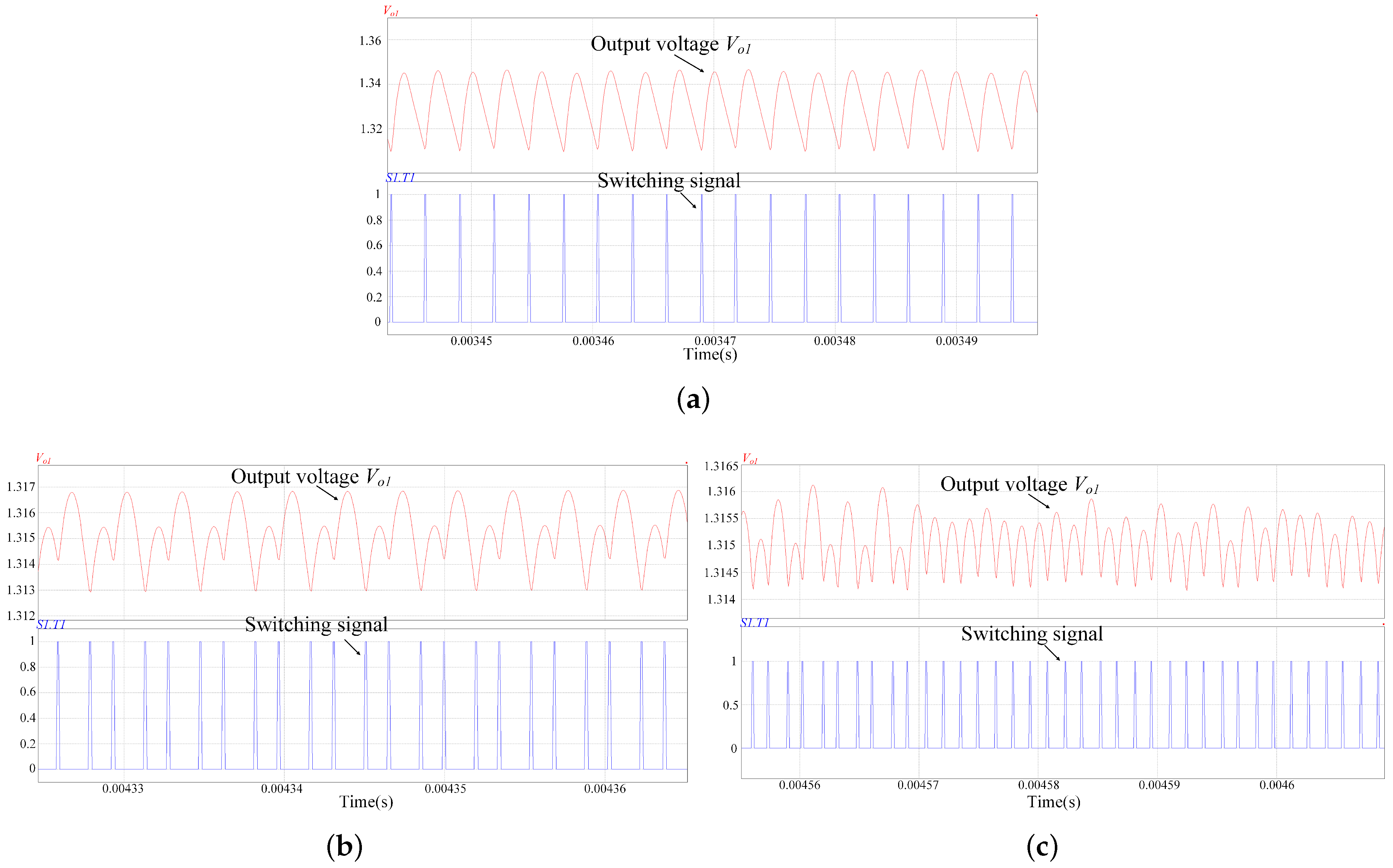
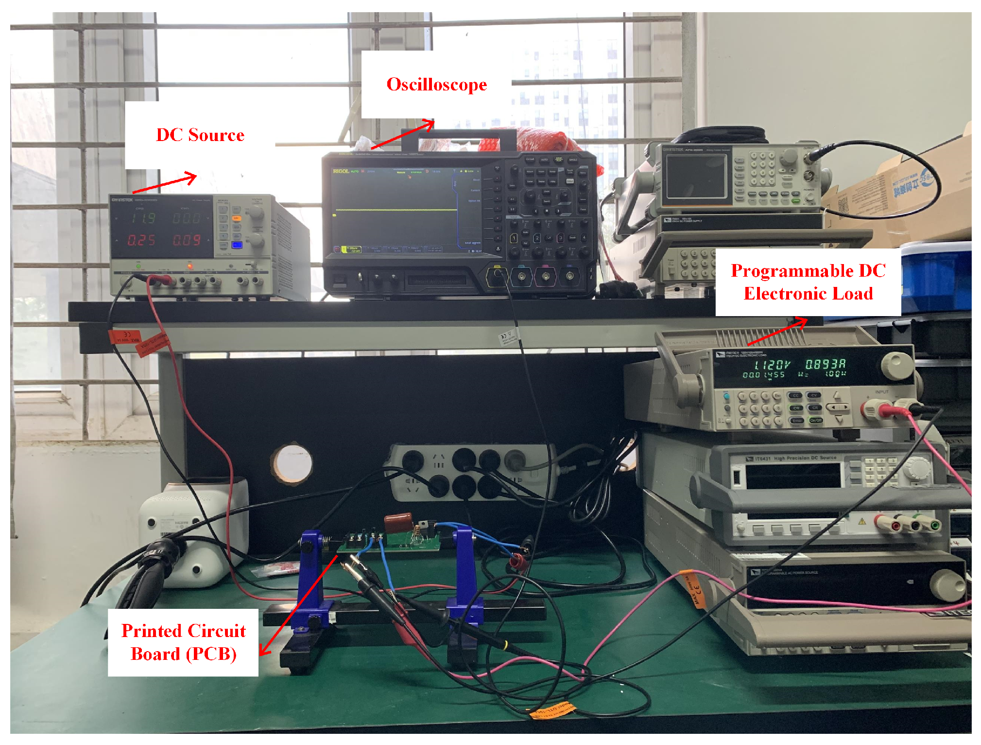
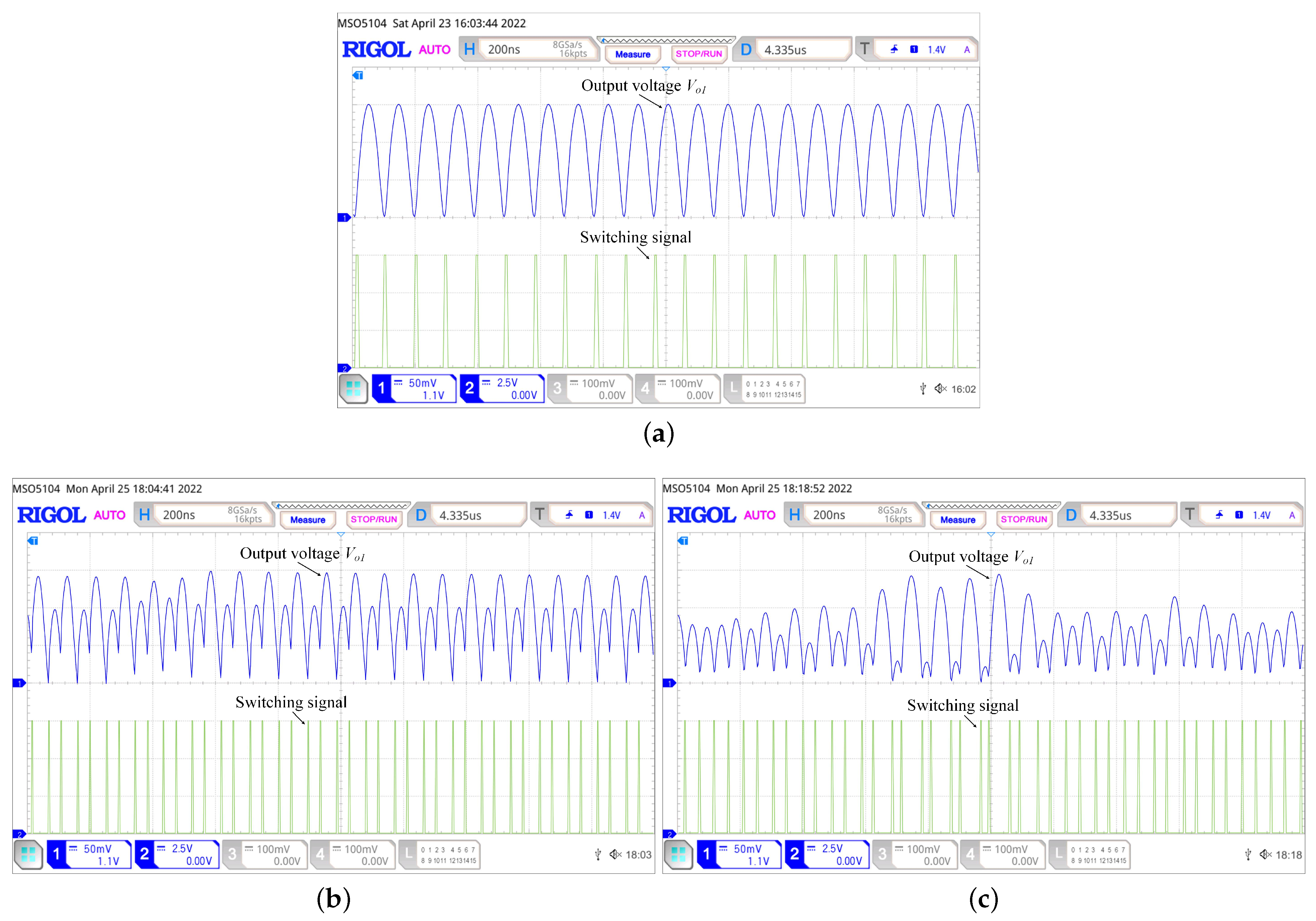
4. Circuit-Level Simulation and Experimental Validations

4.1. Circuit-Level Realization and Simulation

The simulation of the prototype cascaded dc system is constructed in PSIM in Figure 7. The commercial chip LM5085 is used in the subsequent experiment to implement the CMCOTC function, which allows 100% duty cycle operation to achieve low dropout and a wide input voltage range. Hence, an imitation LM5085 chip is established as Figure 7 shows.

Owing to a tightly-regulated power converter behaves as a CPL, which may not behave as an ideal CPL in all situations and this does not present worst situation from a stability point of view [27,28,29]. Thus, a PCMC buck converter with 100kHz switching frequency is regulated to the feeder converter as a CPL in Figure 7. The parameters of the system refer to Table 1. With selected points a, b, and c—shown in Figure 4—as the sample points, the output voltage waveforms are shown in Figure 8 at $P_{CPL}$ = 6 W, 24 W, and 33.1 W, respectively. When $P_{CPL}$ = 6 W, the system is stable. When $P_{CPL}$ = 24 W, the system works in a period-2 subharmonic oscillation state. When $P_{CPL}$ increases to 33.1 W, the system is in a chaotic state.

4.2. Experimental Results

In order to further verify the analysis and simulation, an experimental platform is constructed, as shown in Figure 9, in which a CMCOTC Buck converter is connected with a programmable dc electronic load. While this load works in a constant current mode and the input current is 0∼12 A, the rise rate of the sink current is more than 0.001 A/$\mathsf{\mu }$S but no more than 0.2 A/$\mathsf{\mu }$S, and the fall rate remains between 0.01 A/$\mathsf{\mu }$S and 1.6 A/$\mathsf{\mu }$S. Obviously, in practice, the programmable dc electronic load meets the requirements of the dynamical characteristic of an ideal CPL. The parameters are the same as Table 1 and the simulation. Figure 10 shows the experimental output voltage waveforms of the system.

When $P_{CPL}$ is 6 W, the system works in period-1 stability, which corresponds to Figure 10a. When $P_{CPL}$ = 24 W, a period-2 subharmonic oscillation state can be observed in Figure 10b. As $P_{CPL}$ increases to 33.1 W, a chaotic state occurs and the oscillation is more intense, as shown in Figure 10c.

5. Conclusions

This work discusses a large-signal stability analysis of a dual-stage cascaded dc system from the perspective of load power. In this cascaded system, the control strategies of the feeder and the load converters are different, where a CMCOTC is adopted for the feeder buck converter and a PCMC is employed for the load buck converter. During the modeling process, the load buck converter is equivalent to a CPL for obtaining the discrete-mapping model. Through the use of Lyapunov-type mixed potential theory, an explicit analytical discriminant condition for the stability criterion is deduced, and the full picture of the stable region is depicted in order to guide the design of such systems. According to the results, the system remains stable when the load power is approximately maintained at [6, 24] W. In order to validate the proposed approximation of the region of attraction, the full picture of the discrete-mapping model-based large signal analysis is painted as a reference, in which both a bifurcation diagram and the loci of eigenvalue are contained. Meanwhile, both circuit-level simulations in PSIM and laboratory experiments are carried out to validate the specific boundary conditions.

References

1. Cuzner, R. Does DC Distribution Make Sense? [About This Issue]. IEEE Electrif. Mag. 2016, 4, 2–3. [Google Scholar] [CrossRef]
2. Nordman, B.; Christensen, K. DC Local Power Distribution: Technology, Deployment, and Pathways to Success. IEEE Electrif. Mag. 2016, 4, 29–36. [Google Scholar] [CrossRef] [Green Version]
3. Luo, S. A review of distributed power systems part I: DC distributed power system. IEEE Aerosp. Electron. Syst. Mag. 2005, 20, 5–16. [Google Scholar] [CrossRef]
4. Ji, H.; Xie, F.; Chen, Y.; Zhang, B. Small-Step Discretization Method for Modeling and Stability Analysis of Cascaded dc–dc Converters With Considering Different Switching Frequencies. IEEE Trans. Power Electron. 2022, 37, 8855–8872. [Google Scholar] [CrossRef]
5. Mukherjee, N.; Strickland, D. Control of Cascaded DC–DC Converter-Based Hybrid Battery Energy Storage Systems—Part I: Stability Issue. IEEE Trans. Ind. Electron. 2016, 63, 2340–2349. [Google Scholar] [CrossRef] [Green Version]
6. Mukherjee, N.; Strickland, D. Control of Cascaded DC–DC Converter-Based Hybrid Battery Energy Storage Systems—Part II: Lyapunov Approach. IEEE Trans. Ind. Electron. 2016, 63, 3050–3059. [Google Scholar] [CrossRef] [Green Version]
7. Singh, S.; Gautam, A.R.; Fulwani, D. Constant power loads and their effects in DC distributed power systems: A review. Renew. Sustain. Energy Rev. 2017, 72, 407–421. [Google Scholar] [CrossRef]
8. He, B.; Chen, W.; Mu, H.; Zhan, D.; Zhang, C. Small-Signal Stability Analysis and Criterion of Triple-Stage Cascaded DC System. IEEE J. Emerg. Sel. Top. Power Electron. 2022, 10, 2576–2586. [Google Scholar] [CrossRef]
9. Li, H.; Zhang, Z.; Zhou, Z.; Chu, Z.; Zeng, Y.; Qiu, Z. A Floquet Theory-Based Stability Analysis Method for Cascaded DC-DC Converters by Combining with the Describing Function of PWM Link. In Proceedings of the 2021 IEEE Energy Conversion Congress and Exposition (ECCE), Vancouver, BC, Canada, 10–14 October 2021; pp. 2841–2846. [Google Scholar] [CrossRef]
10. Ding, L.; Wong, S.-C.; Tse, C.K. Bifurcation Analysis of a Current-Mode-Controlled DC Cascaded System and Applications to Design. IEEE J. Emerg. Sel. Top. Power Electron. 2020, 8, 3214–3224. [Google Scholar] [CrossRef]
11. El Aroudi, A.; Haroun, R.; Al-Numay, M.S.; Calvente, J.; Giral, R. Fast-Scale Stability Analysis of a DC–DC Boost Converter With a Constant Power Load. IEEE J. Emerg. Sel. Top. Power Electron. 2021, 9, 549–558. [Google Scholar] [CrossRef]
12. Wu, H.; Pickert, V.; Ma, M.; Ji, B.; Zhang, C. Stability Study and Nonlinear Analysis of DC–DC Power Converters With Constant Power Loads at the Fast Timescale. IEEE J. Emerg. Sel. Top. Power Electron. 2020, 8, 3225–3236. [Google Scholar] [CrossRef] [Green Version]
13. Hu, W.; Yang, R.; Wang, X.; Zhang, F. Stability Analysis of Voltage Controlled Buck Converter Feed From a Periodic Input. IEEE Trans. Ind. Electron. 2021, 68, 3079–3089. [Google Scholar] [CrossRef]
14. Rahimi, A.M.; Emadi, A. An Analytical Investigation of DC/DC Power Electronic Converters With Constant Power Loads in Vehicular Power Systems. IEEE Trans. Veh. Technol. 2009, 58, 2689–2702. [Google Scholar] [CrossRef]
15. Wang, B.; Chen, D.; Chen, C.-J.; Hsiao, S.-F. Stability Prediction of Integrated-Circuit Based Constant ON-Time Controlled Buck Converters. IEEE Trans. Power Electron. 2021, 36, 6838–6849. [Google Scholar] [CrossRef]
16. Brayton, R.K.; Moser, J.K. A theory of nonlinear networks. I. Quart. Appl. Math. 1964, 22, 1–33. [Google Scholar] [CrossRef] [Green Version]
17. Brayton, R.K.; Moser, J.K. A theory of nonlinear networks. II. Quart. Appl. Math. 1964, 22, 81–104. [Google Scholar] [CrossRef] [Green Version]
18. Weiss, L.; Mathis, W.; Trajkovic, L.L. A generalization of Brayton-Moser’s mixed potential function. IEEE Trans. Circuits Syst. I 1998, 45, 423–427. [Google Scholar] [CrossRef] [Green Version]
19. Liu, Z.; Ge, X.; Su, M.; Han, H.; Xiong, W.; Gui, Y. Complete Large-signal Stability Analysis of DC Distribution Network via Brayton-Moser’s Mixed Potential Theory. IEEE Trans. Smart Grid 2022, 2022, 1. [Google Scholar] [CrossRef]
20. Ahmed, M.S.; Fayed, A.A. A Current-Mode Delay-Based Hysteretic Buck Regulator With Enhanced Efficiency at Ultra-Light Loads for Low-Power Microcontrollers. IEEE Trans. Power Electron. 2020, 35, 471–483. [Google Scholar] [CrossRef]
21. Hsu, S.; Chen, C.; Tsai, C. A High Frequency Power and Area Efficienct Charge-Pump-Constant-On-Time Controlled DC-DC Converter Based on Dynamic-Biased Comparator with 50mV Droop and 2us 1% Settling Time for 1.15A/1ns Load Step. In Proceedings of the 2019 IEEE Applied Power Electronics Conference and Exposition (APEC), Anaheim, CA, USA, 17–21 March 2019; pp. 2980–2983. [Google Scholar] [CrossRef]
22. Ming, X.; Xin, Y.; Li, T.; Liang, H.; Li, Z.; Zhang, B. A Constant On-Time Control With Internal Active Ripple Compensation Strategy for Buck Converter With Ceramic Capacitors. IEEE Trans. Power Electron. 2019, 34, 9263–9278. [Google Scholar] [CrossRef]
23. Bizzarri, F.; Nora, P.; Brambilla, A. Closed-Form Operational Boundaries for Buck Converters With Constant On-Time Control. IEEE Trans. Circuits Syst. II Express Briefs 2021, 68, 3331–3335. [Google Scholar] [CrossRef]
24. Tsai, C.; Chen, B.; Li, H. Switching Frequency Stabilization Techniques for Adaptive On-Time Controlled Buck Converter With Adaptive Voltage Positioning Mechanism. IEEE Trans. Power Electron. 2016, 31, 443–451. [Google Scholar] [CrossRef]
25. Li, X.; Zhang, X.; Jiang, W.; Wang, J.; Wang, P.; Wu, X. A Novel Assorted Nonlinear Stabilizer for DC–DC Multilevel Boost Converter With Constant Power Load in DC Microgrid. IEEE Trans. Power Electron. 2020, 35, 11181–11192. [Google Scholar] [CrossRef]
26. Hariharan, K.; Kapat, S.; Mukhopadhyay, S. Constant On-Time Multi-Mode Digital Control with Superior Performance and Programmable Frequency. In Proceedings of the 2019 IEEE Applied Power Electronics Conference and Exposition (APEC), Anaheim, CA, USA, 17–21 March 2019; pp. 1344–1350. [Google Scholar] [CrossRef]
27. Olsson, E. Constant-power rectifiers for constant-power telecom loads. In Proceedings of the 24th Annual International Telecommunications Energy Conference, Montréal, QC, Canada, 29 September–3 October 2002; pp. 591–595. [Google Scholar] [CrossRef]
28. Cupelli, M.; Zhu, L.; Monti, A. Why Ideal Constant Power Loads Are Not the Worst Case Condition From a Control Standpoint. IEEE Trans. Smart Grid 2015, 6, 2596–2606. [Google Scholar] [CrossRef] [Green Version]
29. Lin, G.-Y.; Chen, D.; Chen, Y.-J. The DCM stability issue of voltage regulators using a current-mode constant on-time controller control. In Proceedings of the 2013 IEEE Energy Conversion Congress and Exposition, Denver, CO, USA, 15–19 September 2013; pp. 813–816. [Google Scholar] [CrossRef]
Figure 1. Some typical dual-stage cascaded dc systems [7,8]: (a) Data center dc power supply system. (b) Plug-in hybrid vehicle power supply system. (c) PV-storage integrated grid connected power supply system [7,8].
Electronics 11 04181 g001
Figure 2. The prototype dual-stage cascaded dc system.
Electronics 11 04181 g002
Figure 3. V-I characteristics of CPL and conventional resistive load [7].
Electronics 11 04181 g003
Figure 4. Stability boundary of the system as V i n varies from 8 to 16 V and P C P L varies from 0 W to 35 W.
Electronics 11 04181 g004
Figure 5. Bifurcation diagram of P C P L from 5 to 35 W.
Electronics 11 04181 g005
Figure 6. Loci of eigenvalues: (a) P C P L varies from 5.8 to 5.5 W. (b) P C P L varies from 23.2 to 23.5 W. (c) P C P L varies from 32.8 to 33.1 W.
Electronics 11 04181 g006
Figure 7. Schematic of CMCOTC buck converter with CPL in simulation.
Electronics 11 04181 g007
Figure 8. Simulation waveforms of the system with varying: (a) P C P L = 6 W. (b) P C P L = 24 W. (c) P C P L = 33.1 W.
Electronics 11 04181 g008
Figure 9. Experimental platform of the system.
Electronics 11 04181 g009
Figure 10. Experimental waveforms of the system with varying: (a) P C P L = 6 W. (b) P C P L = 24 W. (c) P C P L = 33.1 W.
Electronics 11 04181 g010