Handcrafted Deep-Feature-Based Brain Tumor Detection and Classification Using MRI Images

Abstract

An abnormal growth of cells in the brain, often known as a brain tumor, has the potential to develop into cancer. Carcinogenesis of glial cells in the brain and spinal cord is the root cause of gliomas, which are the most prevalent type of primary brain tumor. After receiving a diagnosis of glioblastoma, it is anticipated that the average patient will have a survival time of less than 14 months. Magnetic resonance imaging (MRI) is a well-known non-invasive imaging technology that can detect brain tumors and gives a variety of tissue contrasts in each imaging modality. Until recently, only neuroradiologists were capable of performing the tedious and time-consuming task of manually segmenting and analyzing structural MRI scans of brain tumors. This was because neuroradiologists have specialized training in this area. The development of comprehensive and automatic segmentation methods for brain tumors will have a significant impact on both the diagnosis and treatment of brain tumors. It is now possible to recognize tumors in photographs because of developments in computer-aided design (CAD), machine learning (ML), and deep learning (DL) approaches. The purpose of this study is to develop, through the application of MRI data, an automated model for the detection and classification of brain tumors based on deep learning (DLBTDC-MRI). Using the DLBTDC-MRI method, brain tumors can be detected and characterized at various stages of their progression. Preprocessing, segmentation, feature extraction, and classification are all included in the DLBTDC-MRI methodology that is supplied. The use of adaptive fuzzy filtering, often known as AFF, as a preprocessing technique for photos, results in less noise and higher-quality MRI scans. A method referred to as “chicken swarm optimization” (CSO) was used to segment MRI images. This method utilizes Tsallis entropy-based image segmentation to locate parts of the brain that have been injured. In addition to this, a Residual Network (ResNet) that combines handcrafted features with deep features was used to produce a meaningful collection of feature vectors. A classifier developed by combining DLBTDC-MRI and CSO can finally be used to diagnose brain tumors. To assess the enhanced performance of brain tumor categorization, a large number of simulations were run on the BRATS 2015 dataset. It would appear, based on the findings of these trials, that the DLBTDC-MRI method is superior to other contemporary procedures in many respects.

1. Introduction

Brain tumors are among the most dangerous types of brain diseases that can develop as a result of abnormal cell growth within the skull. There are two types of brain tumors: primary tumors and secondary tumors. Primary brain tumors account for 70% of all tumors and spread only in the brain, whereas secondary brain tumors form in other organs before migrating to the brain, such as the breast, kidney, and lung. According to a National Brain Tumor Foundation (NBTF) study, approximately 29,000 cases of primary brain tumors are diagnosed in the United States each year, resulting in the deaths of 13,000 people [1]. According to R.J. Young [2], roughly 42,000 people in the United Kingdom die each year from primary brain tumors. Gliomas, meningiomas, and pituitary tumors are the three most common forms of brain tumors. Gliomas are caused by the unregulated growth of glial cells, which constitute approximately 80 percent of the brain’s tissue. This primary cancer has the greatest death rate of any cancer. Meningioma tumors form in the spinal cords meninges, the membrane that protects the brain. The pituitary tumor, on the other hand, develops within the pituitary gland. This gland produces many important hormones. Although pituitary tumors are benign, they can induce hormonal imbalances and irreversible visual loss. It is critical to obtain an accurate and timely diagnosis of brain tumors [3] to prevent patients from negative consequences. Multiple imaging techniques can be used to diagnose brain tumors, each with a slightly different focus. Three of the most used tools are computed tomography (CT), magnetic resonance imaging (MRI), and ultrasound [4]. MRI, or magnetic resonance imaging, is the most widely used non-invasive imaging method. As opposed to X-rays, MRI scans do not produce any hazardous ionizing radiation. In addition, it may provide a variety of modalities by employing different parameters including FLAIR, T1, and T2 to create clear images of soft tissues [5].

The challenge of correctly identifying a tumor’s type is challenging because tumors typically differ in form, severity, size, and location. Typically, the medical staff carefully mark out the tumor locations in the photos after visually inspecting them. Tumor borders are typically masked by healthy tissues around them. Therefore, optical-inspection-based manual tumor identification is labor-intensive and fraught with opportunities for error. Furthermore, the radiologist’s experience is crucial for manual tumor detection [6]. It is important to remember that the distinct grayscales shown in MRI scans are not visible to the human eye. It depends on the radiologist’s experience to distinguish between malignant and benign lesions using MR images. To distinguish between malignant and benign lesions for non-experts, we developed a simplified systematic MRI approach using depth, size, and heterogeneity on T2-weighted MR images (T2WI), and we assessed its diagnostic efficacy. In [7,8], we evaluated 13 pre-trained deep convolutional neural networks and 9 ML classifiers on three brain tumor datasets (BT-small-2c, BT-large-2c, and BT-large-4c). The experimental results indicate that from our architecture, (1) the DenseNet-169 deep feature alone is a good choice if the MRI dataset is small and there are two classes (normal, tumor), (2) the ensemble of DenseNet-169, Inception V3, and ResNeXt-50 deep features is a good choice if the MRI dataset is large and there are two classes (normal, tumor), and (3) the ensemble of DenseNet-169, ShuffleNet V2, and MnasNet deep is a good choice with the classes normal, glioma tumor, meningioma tumor, and pituitary tumor. The traditional machine-learning-based approaches have the drawback of requiring the extraction of features manually. To classify photos, first, the features that were collected from the training set are retrieved [9].

Brain tumor classification techniques are classified as machine learning (ML) or deep learning (DL) methods. Before classification, ML-based systems use time-consuming and error-prone handcrafted feature extraction and manual segmentation. To discover optimal feature extraction and segmentation algorithms for proper tumor identification, these strategies typically necessitate the assistance of a trained expert who can choose the most appropriate feature extraction and segmentation algorithms for accurate tumor detection. Because of this, there is inconsistency in the performance of these systems when dealing with larger datasets [10]. Meanwhile, DL-based algorithms have proven to be effective in many areas, including the interpretation of medical images, and take care of these tasks automatically. Convolutional neural networks (CNN) are popular deep learning models because of their reliable performance and weight-sharing architecture. High-level and low-level features can be automatically extracted from the training data. Academics and scientists are thus becoming increasingly interested in these phenomena [11,12].

This research integrates deep data collected by three popular CNNs to propose an automated strategy for detecting and classifying brain tumors (AlexNet, ResNet18, and GoogLeNet). The method has multiple applications for detecting and classifying brain tumors. During feature fusion, many feature vectors, both low-level and high-level, are combined into a single feature vector.

Thus, the model’s discriminative performance has improved since it no longer relies on a single feature vector. For accurate tumor classification, it is necessary to create informative and discriminative features from MRIs, and this in turn pushes the adoption of a feature fusion technique. The correct classification of tumors depends on this. We put our model through its paces using a well-known dataset on brain tumors and several quantitative characteristics. To demonstrate the efficacy of the suggested method, we used multiple quantitative measures to assess our model on a well-known brain tumor dataset [13]. The following is a list of the key contributions that the proposed system will make.

In this paper, the authors present a completely automated hybrid technique for classifying different types of brain tumors by using (a) ML classifiers and (b) convolutional neural network (CNN) models trained with transfer learning for deep feature extraction. This approach was created to help with the challenging task of precisely detecting brain tumors.

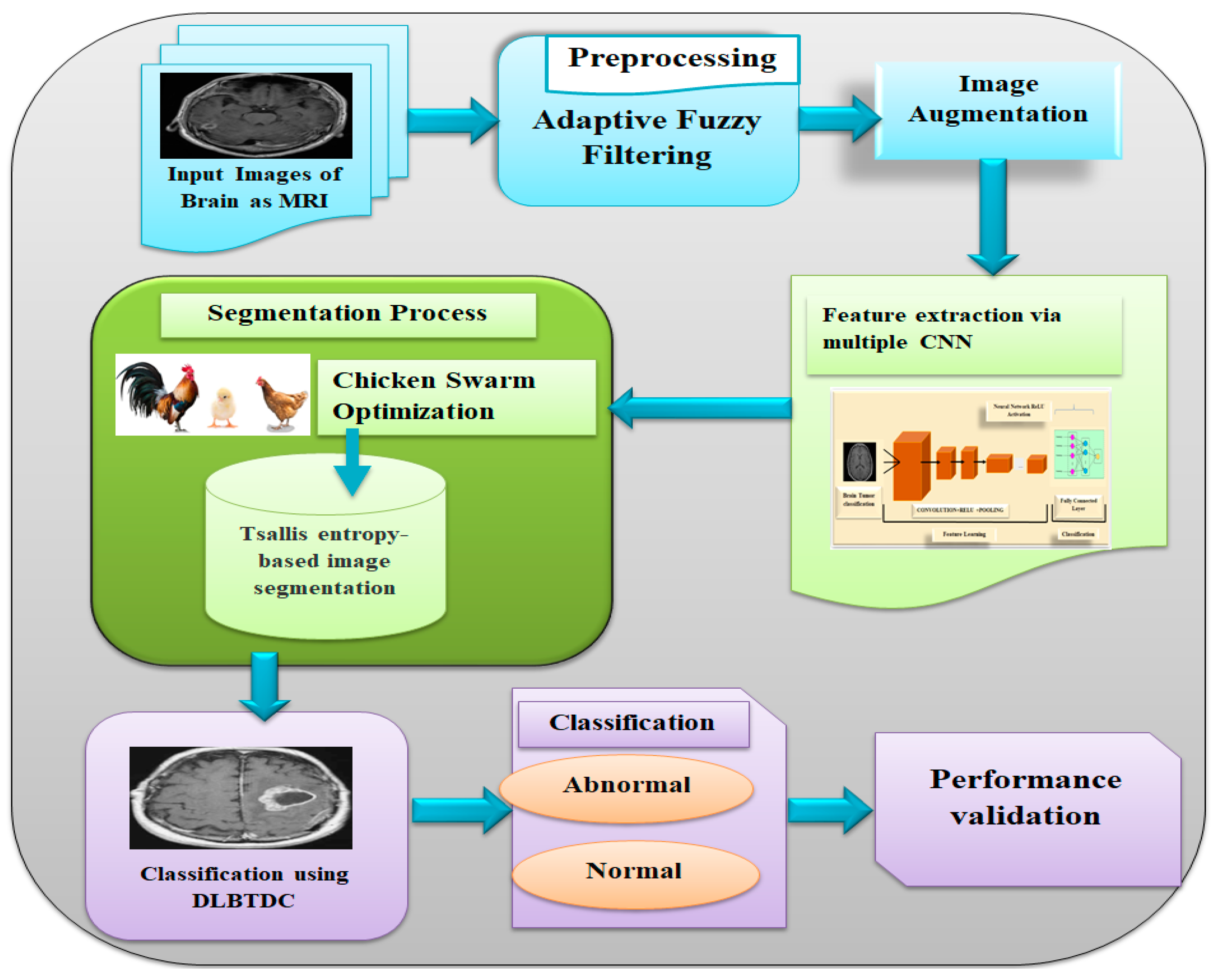
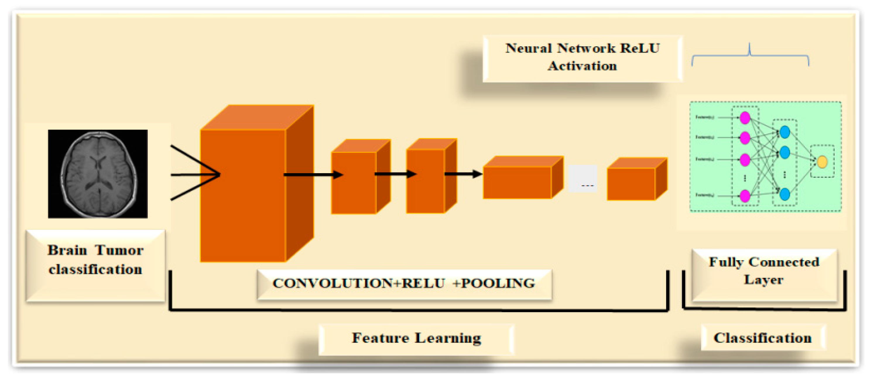
The proposed method consists of six core steps: (a) adaptive fuzzy filtering (AFF); (b) brain cancer diagnosis using MR images, which requires (c) a large-scale dataset extension and (d) feature extraction using multiple convolutional neural networks (CNNs), such as ResNet 18; (e) fusion of deep feature vectors, which provides state-of-the-art performance, and (f) classification of different tumor types.

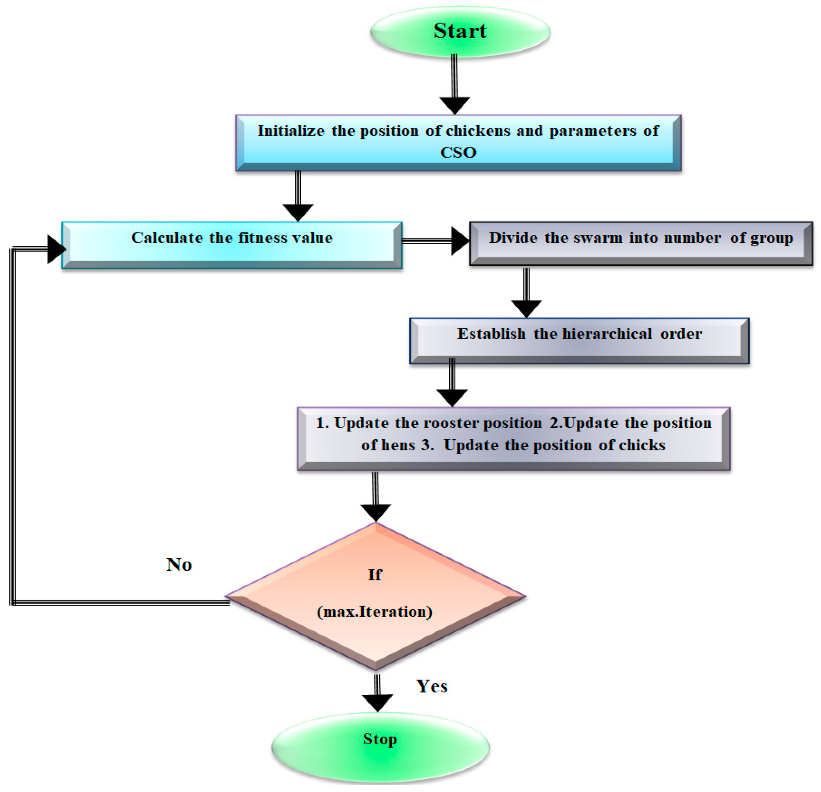
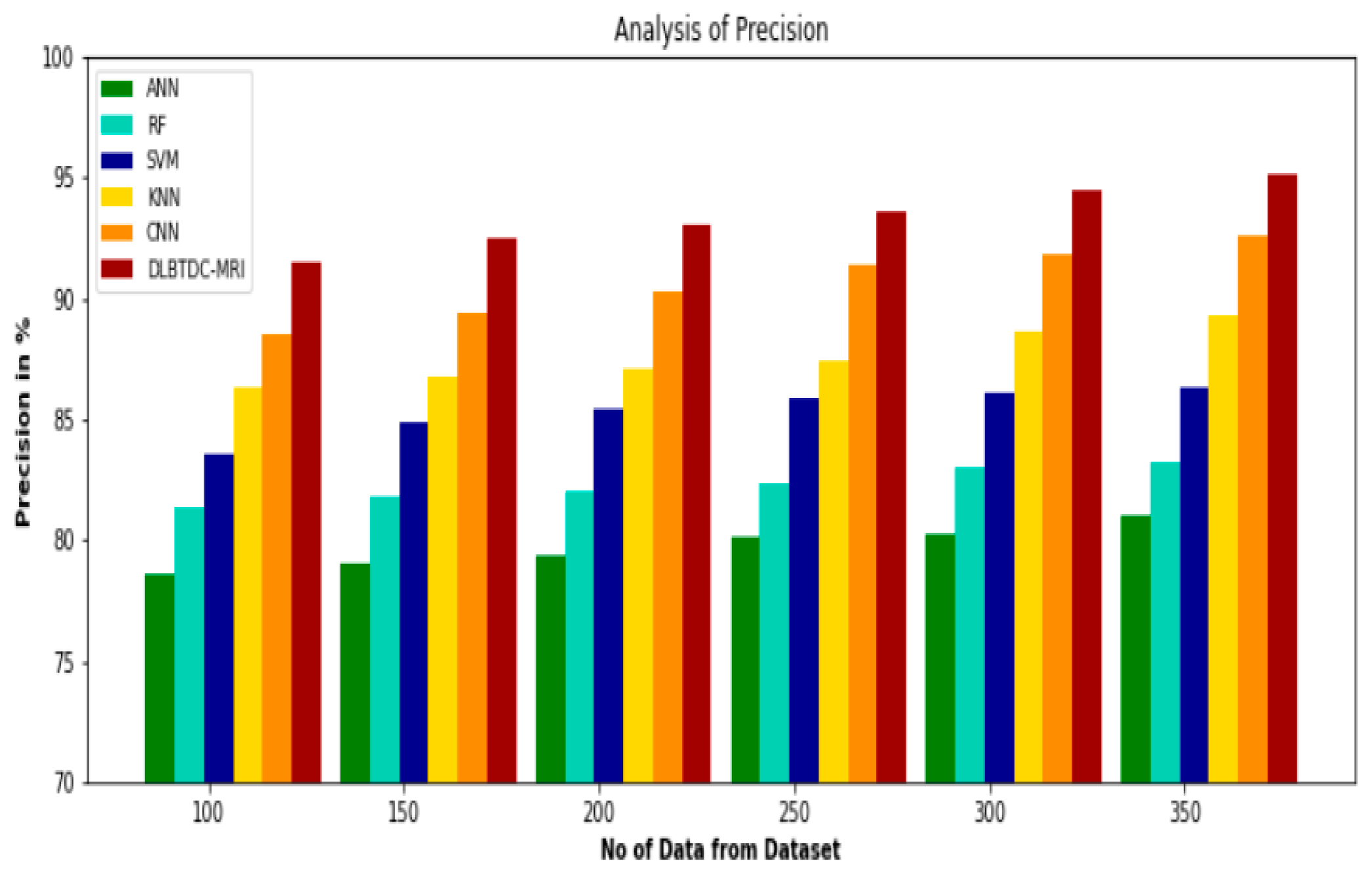
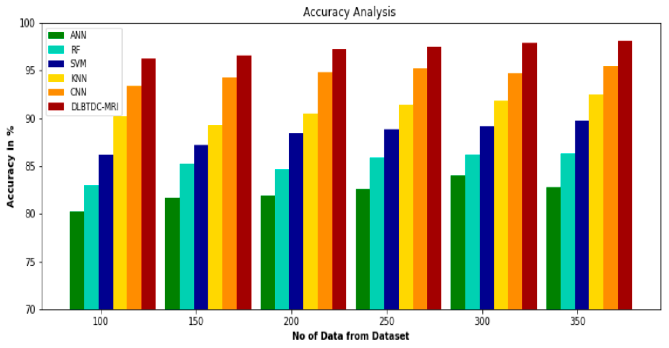
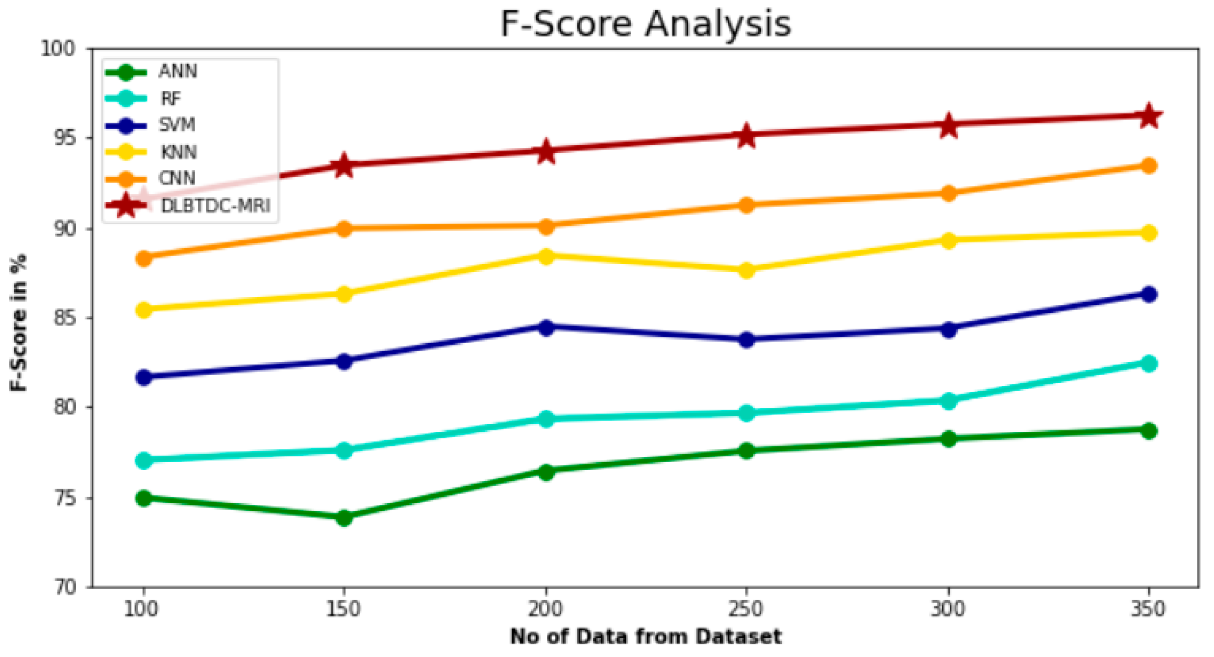
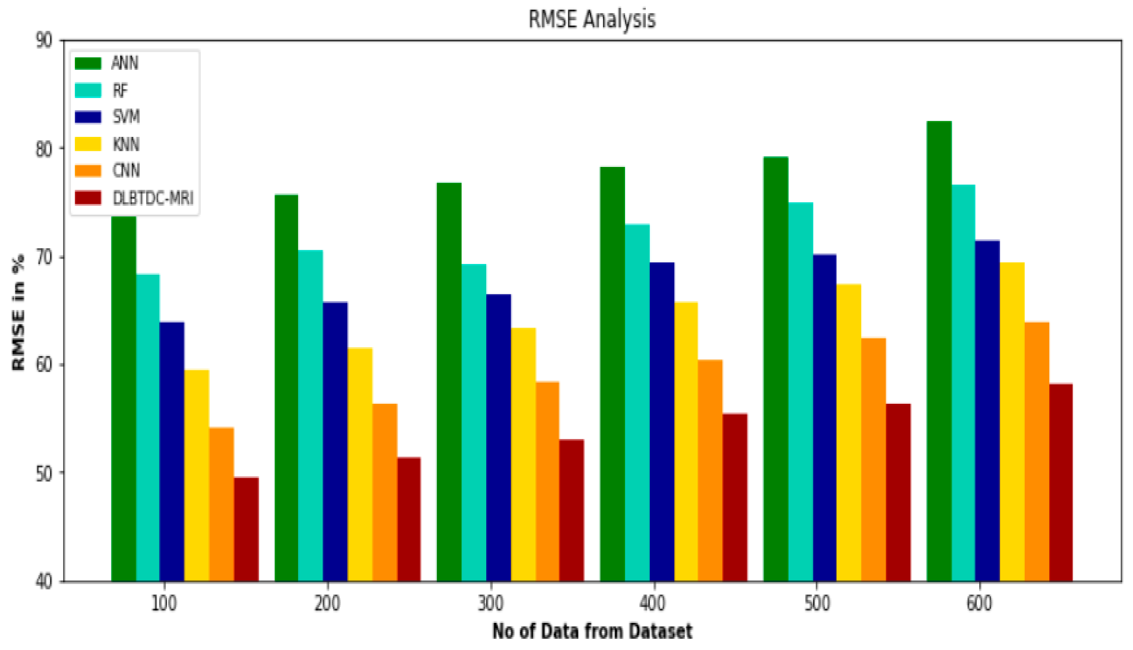
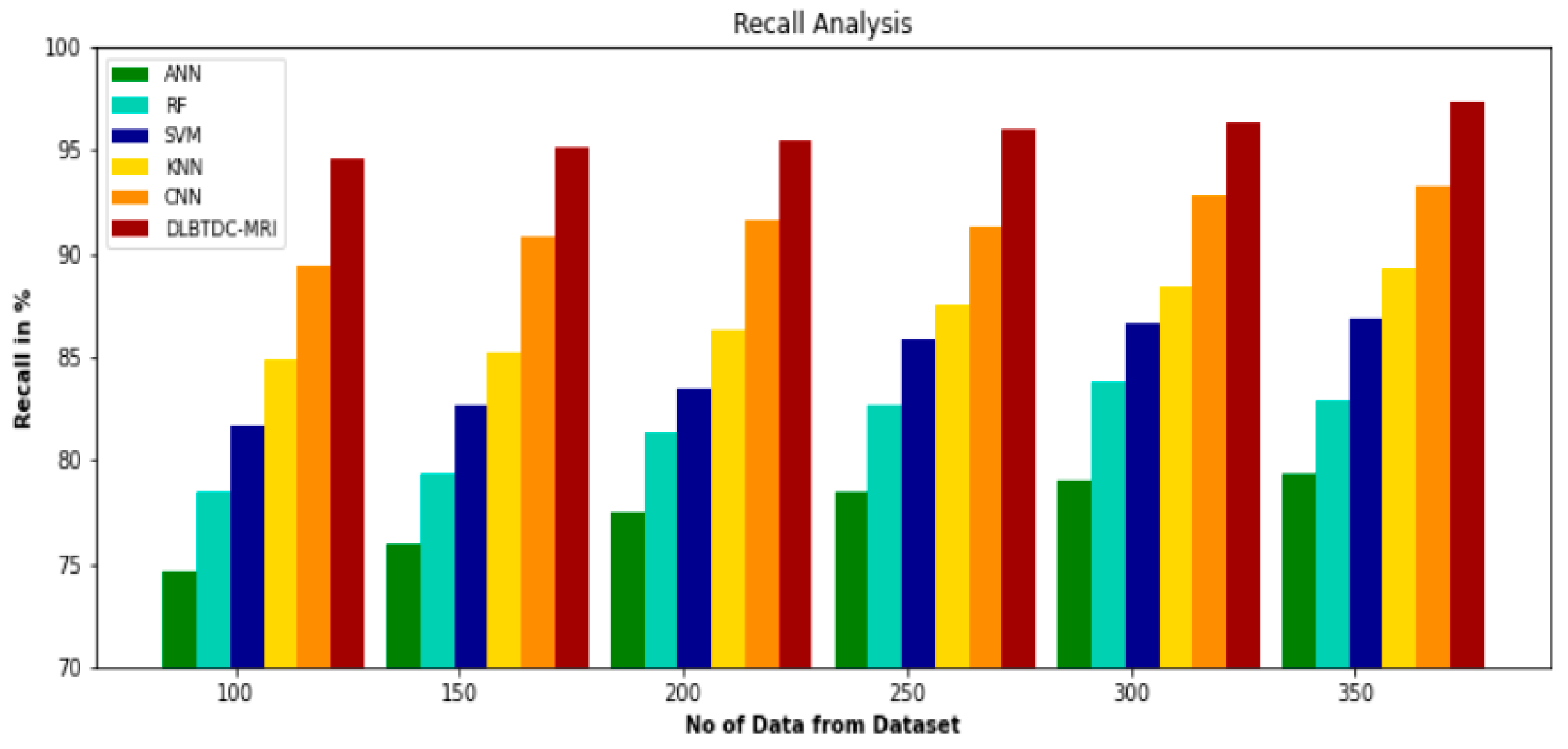
A classifier based on DLBTDC-MRI and CSO can detect brain tumors. Numerous simulations were conducted using the BRATS 2015 dataset to examine the enhanced performance in classifying brain tumors.

An overview of the rest of the paper follows. The literature review’s research is dissected in Section 2. Section 3 describes the DLBTDC-MRI approach that has been proposed. Experiments and findings are discussed in detail in Section 4. The work that has been proposed is concluded, and future studies are suggested, in Section 5.

2. Literature Survey

A CNN model was presented by Ayadi et al. [14] which carries out the necessary comparison both before and after the data augmentation is applied. They demonstrated that by adding additional data to the model that they constructed, the accuracy of the model could be improved. They used three different data sets to test how well it worked and found that it could find 98.43% of pituitary tumors, which is a big step forward in the field.

Jude Hemanth [15] et al. presented a model for diagnosing brain illnesses using MRI by resolving the limitations of ANNs regarding the amount of time needed for convergence. They accomplished this by using modified versions of the Counter Propagation Neural Model (CPN) and the Kohonen Neural Network (KNN), referred to as MCPN and MKNN, respectively. When they set out to design this model, their primary goal was to reduce the number of iterations in the ANN model so that it could solve the convergence rate; after modification, MKNN and MCPN had accuracy rates of 95% and 98%, respectively. The number of ANN model iterations required to determine the convergence rate was kept to a minimum.

Nayak et al. [16] suggested using models where there is no segmenting or preprocessing. The data were put into groups with the help of multiple logistic regression. A CNN model that had already been trained and pictures that were cut up were used in the suggested method. The model was tested with three sets of data. Several data augmentation methods were used to improve accuracy. This method was tried out on both the unique information set and the extended information set. Compared to studies that have come before, the results are rather convincing.

To improve the degree to which the CAD system interacts with the user, Sachdeva et al. [17] suggested a method for locating tumor foci. They utilized a wide variety of datasets to assess the accuracy of their suggested model. The first set of data had three different types of cancer, while the second had five different categories. Two novel models, the GA-SVM and the GA-ANN, were produced by applying a genetic algorithm (GA) to both the SVM and the ANN models.

Both of these vehicles qualify as hybrids. Following the execution of the suggested technique, the SVM model’s accuracy increased from 79.3% to 91%, while the ANN model’s accuracy increased from 75.6% to 94%.

Mzoughi et al. [18] used the BRATS 2018 dataset’s complete volumetric T1-Gado MRI sequence to construct a 3D CNN architecture for classifying glioma brain tumors into low-grade gliomas (LGG) and high-grade gliomas (HGG). Based on a deep neural network and a three-dimensional convolutional layer, the design uses small kernels and lower weights to take into consideration both local and global contexts. A total of 96.49 % of inputs were correctly processed by the system.

Maqsood et al. [19] developed an edge discovery and U-NET prototype-based approach for detecting brain tumors. This technique may be found in their publication. The framework for tumor segmentation enhances picture contrast and makes use of fuzzy logic for edge detection. By first extracting features from fading sub-band pictures and then categorizing those structures, the U-NET architecture can determine whether or not a meningioma is present in a patient’s brain imaging.

According to Afshar et al. [20], the classification of brain tumors (CapsNet) will use a member network capsule CNN architecture. The technique known as CapsNet makes use of the spatial interaction that occurs between the tumor and the tissues that surround it. The segmented tumor produced results that were 86.56 % correct, whereas the picture of the brain that had not been altered produced results that were 72.13 % accurate.

Abiwinanda et al. [21] suggest either studying the canonical CNN model without making any changes or developing CNN while simultaneously altering the CNN layers by either increasing or decreasing the total number of layers. This led to the creation of seven separate CNN architectures, each with a unique set of layers. They found that their second design (two layers for each difficulty level, a starting point, and maximum pooling) had the highest training accuracy (98.51%).

Khan et al. [22] proposed a deep-learning-based hierarchical categorization system for brain tumors. In this study, researchers used MRI images from the Kaggle dataset to reach a classification accuracy of 92.13%. However, due to the low overall accuracy, the approach must be evaluated before being used in clinical settings for brain tumor categorization.

Ghassemi et al. [23] proposed a pretraining-focused model and then used it with CNN. In this manner, the primary emphasis is placed on pretraining the model using various publicly available datasets, after which the model is applied. In the focus prototype, the SoftMax replaced the CNN and fully connected layers, and the ensuing prototype was validated using the primary dataset T1, which contained three distinct forms of a tumor, and obtained a 95.6% accuracy rate.

3. Proposed System

In Figure 1, we see a block diagram of the proposed DLBTDC-MRI method. The input, which consists of MRI scans of the patient’s brain, is then preprocessed using an adaptive fuzzy filtering algorithm, as the graphic makes abundantly evident. After being preprocessed, the data is then transferred to be used for picture enhancement. Image augmentation is a method that involves modifying the already-present data to generate additional data for the process of training a model. The technique of artificially increasing the available dataset to train a deep learning model is referred to as “dataset augmentation”. The information is then fed into CNN so that features can be extracted. One type of artificial neural network capable of recognizing and analyzing images is the convolutional neural network (CNN). It was made to process pixel information in a specific way.

The data, after preprocessing and feature extraction, are sent for a segmentation process that involves Tsallis entropy-based image segmentation using the Chicken Swarm Optimization algorithm. The segmented images are then classified using the DLBTDC algorithm, which categorizes the images as being either regular or irregular. The final data are then checked to show that it works better than the other methods.

3.1. Data Preparation

3.1.1. Adaptive Fuzzy Filtering

In the proposed filter’s detection phase, the two local maxima, Lsalt and Lpepper, are sought. The search will be oriented to the center of the picture matrix, and it will be responsive to direction [24,25,26,27]. In an 8-bit integer representation of an image, Lsalt is set to 255, and Lpepper is set to 0.

The noisy pixel will be identified by the aforementioned range of intensities. A mask M(i,j) is made to identify the position of the noisy pixel:

$$\begin{array}{l}N(i,j)=\{0, x(i,j)=Lsalt or Lpepper\\ \{1 Otherwise\end{array}$$

(1)

where X(i,j) is the pixel at position (i,j) with intensity x, N(i,j) = 1 denotes noise-free pixels to be kept from the noisy picture, and N(i,j) = 0 specifies noise pixels. The noisy image will consist of the pixels with the intensity x.

3.1.2. The Filtering Stage

During filtering, a 3 × 3 scan is performed on the noisy pixels by comparing the central pixel to the surrounding pixels [28,29,30,31]. For a 33-pixel scan, the algorithm takes the center pixel into account, which leads to the following:

$$ld(i,j)=\left|X(i+k,j+1)-X(i,j)\right| with(i+k,j+1)\ne (i,j)$$

(2)

The absolute luminance difference is denoted by ld(i,j), while the noisy pixel is denoted by X(i,j).

Next, a scanning technique is conducted by averaging four neighbouring pixels against the original three. This “merging” scanning is performed to get rid of the noisy pixels that the 3 × 3 scanning process left behind. When performing merge scanning, the algorithm is used.

The absolute luminance difference is denoted by ld(i,j), the merge scanning is denoted by f(i,j), and the threshold is denoted by (i,j). Improving the image’s edges and textures comes next after the noise has been reduced.

3.2. Image Augmentation

Due to the small number of MRI [32,33,34,35] samples contained in the dataset that was used for this investigation, the preprocessed images had to be artificially enhanced using a variety of different approaches, all of which are described and illustrated in Figure 1. Because of the uneven distribution of classes, models have a proclivity to classify fresh samples as majority class types; thus, this issue can be mitigated by artificially enriching the dataset. A left-to-right mirror effect was achieved by adding salt-and-pepper noise with a density (d) of 0.003, inverting the images along the x-axis, and rotating them 45 degrees via bilinear interpolation. In this type of interpolation, a pixel’s output value is the weighted average of the values of the pixels in its 2-by-2 neighborhood.

3.3. Feature Extraction

3.3.1. Classification of CNN

A neuronal convolutional network [36,37,38,39] was used here. Academics value CNN because of their persistent success, which has motivated them to tackle previously impossible problems. In recent years, scientists have created a plethora of CNN designs to address a wide range of challenges in a wide range of disciplines, such as medical image recognition. CNN consists of numerous stacked layers [40,41]. The architecture of a CNN is composed of two primary parts: (i) feature extraction, which uses convolutional layers to learn features, and (ii) classification, which employs a fully connected (FC) layer to classify an image [42]. In a typical CNN, the feature extraction module comes first, followed by the classification module. The general CNN architecture is shown in Figure 2.

3.3.2. Residual Network

It is generally accepted that deeper networks have the potential to perform better than their shallower counterparts [43,44,45,46]. However, beyond a certain depth, a saturation point is reached in network performance when assessing deep learning techniques on medical images. When it comes to brain tumor segmentation, for instance, the shallower network outperforms the deeper one. Overfitting is typically to blame for this degeneration [47,48,49,50]. The lack of a large enough dataset in medical imaging is a contributing factor. In addition, standard deep networks for natural image identification are unfit for medicinal picture classification due to the unique characteristics of these images, such as the subtle changes in appearance between the target and the non-target [51,52,53,54]. In this paper, we adopted the residual system as the feature removal system to solve the aforementioned issues. It is possible to present the optimization as due to the “skip connection” in the residual network.

G(m) = H(m) + m,

(3)

m is the value of the input, G(m) is the value of the projected output, and H(m) is the value of the learning target. The stacked layers will be trained to approximate a residual function rather than G(m), which will be approximated by the model.

H(m) = G(m) − m.

(4)

As a consequence of this, it would be simpler for the network to approximate the residual to be equal to zero as opposed to fitting an identity mapping using some nonlinear layers. Additionally, residual networks can hasten the progression of gradients during back-propagation.

3.4. Chicken Swarm Optimization

CSO is an optimization method that takes its cues from nature, namely the structure and behaviour of a chicken swarm [55,56,57]. Each group of chicken swarms has one rooster, many hens, and several chicks [58,59,60,61,62]. As each type of chicken is subject to its own unique set of physical laws, a certain pecking order has developed among the species [63,64,65,66].

3.4.1. Solution Encoding

To determine the best tumor classification solution, a vector representation of that solution was used.

3.4.2. Fitness Function

To select the healthiest hens, chicks, and roosters, the fitness function is measured. Each rooster in a flock of chickens is considered the de facto leader because he has the highest fitness score. Chicks are designated as the chickens with the lowest fitness scores, while the others are classified as adults. On the other hand, the hen chooses at random which of her groups of chicks she will raise as her own. An equation like the one below is used to determine the fitness function:

$$P_a=\frac{1}{c}{\displaystyle \sum _{z=1}^c{O}_d-\vartheta }$$

(5)

where the actual output of the classifier is represented by $O_d$ and the anticipated output is represented by $\vartheta$. An explanation of the algorithmic procedures that are incorporated into the proposed CSO algorithm is presented below.

3.4.3. Initialization of Population

To simplify, let us say we have a population with the following characteristics: D is the number of roosters, S is the number of hens, Y is the number of chicks, and Z is the number of mother hens. The position of each of the B number of virtual chickens is represented by $a_{y,z}^s\left(y\in \left[1,\dots ,B\right],z\in \left[1,\dots ,B\right]\right)$ with a period step of r, and they are searching for their food in the H-dimensional space. In this establishment, the roosters are selected from the best of the D chickens, while the chicks are selected from the poorest of the Y chickens.

3.4.4. Fitness Evaluation

Chickens are sorted into a hierarchy based on their fitness scores, and a random process is used to determine the association among the hens and the chicks in the flock.

3.4.5. The Rooster’s Current Status

At feeding time, the roosters with the highest fitness levels are prioritized. Chickens in a flock will follow the rooster to get food, but they will aggressively defend their meal from the other fowl in the flock. Chickens are known to randomly raid their neighbors’ feeders. For convenience’s sake, roosters with the highest fitness values look for food in more places than roosters with the lowest fitness values. As a result, the current rooster equation is written as follows:

$$a_{y,z}^{s+1}=a_{y,z}^s\times \left(1+\varpi \left(0,e^2\right)\right)$$

(6)

$$a_{y,z}^{s+1}=a_{y,z}^s+a_{y,z}^s.\varpi \left(0,e^2\right)$$

(7)

$$a_{y,z}^{s+1}-a_{y,z}^s=a_{y,z}^s.\varpi \left(0,e^2\right)$$

(8)

where $\varpi \left(0,e^2\right)$ calls for a Gaussian distribution with a mean of 0 and a standard deviation of $e^2$. Despite the fact that the factional theory has been applied to the most recent version of the rooster equation, the aforementioned Equation (6) has been normalized as:

$$T^{\alpha }\left[a_{y,z}^{s+1}\right]=a_{y,z}^s.\varpi \left(0,e^2\right)$$

(9)

Equation (7) needs to be rewritten in the form of the standard equation, which looks like this:

$$a_{y,z}^s\varpi \left(0,e^2\right)=a_{y,z}^{s+1}-\alpha a_{y,z}^s-\frac{1}{2}{a}_{y,z}^{s-1}-\frac{1}{6}\left(1-\alpha \right)a_{y,z}^{s-2}-\frac{1}{24}\alpha \left(1-\alpha \right)\left(2-\alpha \right)a_{y,z}^{s-3}$$

(10)

$$a_{y,z}^{s+1}=a_{y,z}^s\left(\alpha +\varpi \left(0,e^2\right)\right)+\frac{1}{2}\alpha a_{y,z}^{s-1}+\frac{1}{6}\left(1-\alpha \right)a_{y,z}^{s-2}+\frac{1}{24}\alpha \left(1-\alpha \right)\left(2-\alpha \right)a_{y,z}^{s-3}$$

(11)

Here, the term $e^2$ is expressed as

$$e^2=\left\{\begin{array}{l}1, if f_y\le f_{m } ;m\in \left[1,B\right],m\ne y\\ \exp \left(\frac{\left(f_m-f_y\right)}{\left|f_y\right|+z}\right), otherwise\end{array}\right\}$$

(12)

where z is the minimal continuous, m is a rooster index chosen from the rooster collection, f is the fitness value of the linked a, and d is the order of the derivative between 0 and 1.

3.4.6. Position Update of Hen

When they need food, the hens follow the lead of the rooster in their flock. In most cases, the hen will also help herself to the food that other chickens have stumbled upon by accident. Hens that are dominant over their peers have a greater number of benefits. As a result, the equation used to express the update for hen is as follows:

$$a_{y,z}^{s+1}=a_{y,z}^s+L1 \times e \times \left(a_{s1,z}^s-a_{y,z}^s\right)+L2\times e \times \left(a_{s2,z}^s-a_{y,z}^s\right)$$

(13)

where the terms L1 and L2 are denoted by the following:

$$L1=\exp \left(\frac{\left(f_y-f_{s1}\right)}{abs\left(f_y\right)+z}\right)$$

(14)

$$L2=\exp \left(f_{s2}-f_y\right)$$

(15)

where e is an arbitrary value between 0 and 1. s1 assigns the yth hen group mate to s1 ∈ [1, …, B]. Furthermore, s2 is the chicken index (either hen or rooster), which is chosen at random from the swarm so that s2 ∈ [1, …, B] and $s1\ne s2$ exist.

Obviously, $f_y>f_{s1}$, and $f_y>f_{s2}$, thus L2 < 1 < L1. When L1 = 0, then $y^{th}$ hen forages for food, followed by other animals. Hens are known to try to steal food from other chickens when there is more space between them. A case of linguistic wholeness emerges among the chickens as a result of the dissimilarity between L1 and L2. When L2 is at zero, the 90 hen forages only inside its home range. The alpha hens are the most likely to show submission to the other hens during feeding time.

3.4.7. Chicken Status Report

The chicks seek food near the hen or their mother, with the more dominant chicks having an advantage. As a result, the chicks will wander about the mother in order to search for food, as demonstrated by the following equation:

$$a_{y,z}^{s+1}=a_{y,z}^s+J\times \left(a_{u,z}^s-a_{y,z}^s\right)$$

(16)

where $a_{u,y}^s$ denotes the position of $y^{th}$ chick’s mother, such that u ∈ [1,B], and J(J ∈ [0, 2]) This is the structure which requires that the chick follows their mother foraging for food. Therefore, the parameter J of each chick chooses a random number between 0 and 2 for each value. Figure 3 shows the flowchart of the CSO optimization.

3.4.8. Tsallis Entropy

Our discussion will be conducted using a separate set of probabilities denoted by the symbol “pi,” composed with the random variable I because images are made up of pixels that have distinct shades of grey. The following serves as a condition for the probabilities: ${\displaystyle {\sum }_i{R}_i}$=1.

The Tsallis entropy can be described as for any parameter S in the real world:

$$T_S=\frac{m}{s-1}\left(1-{\displaystyle \sum _i{R}_i^s}\right)$$

(17)

The “entropic index” can be defined as the parameter S that appears in Equation (1); m is a constant that is predetermined to be equal to 1 during the picture processing. In the limit, when S1 is equal to zero, the Boltzmann–Gibbs–Shannon (BG) entropy is restored. The BG figures indicate that the systems in question are substantial. Let us take into consideration a physical system that has been broken down into two independent systems, C and D, both of which have a joint probability: BGS entropy is additive, and R (C, D) = R(C) p(D).

$$T_{BG}(C,D)=T_{BG}(C)+T_{BG}(D)$$

(18)

In the case the Tsallis entropy is evaluated, we have:

$$T_S(C,D)=T_S(C)+T_S(D)+(1-S)T_S(C)T_S(D)$$

(19)

In the boundary of $S\to 1$, we have the predictable additivity of entropy. In the case q < 1, the entropy is sub-extensive: $T_S(C,D)<T_S(C)+T_S(D)$ When q = 1, it is extensive and when q > 1, it becomes super extensive, being $T_S(C,D)>T_S(C)+T_S(D)$. Let us also point out that the entropy proposed by Tsallis is related to the entropy proposed by Alfred Rényi, which can be described as [10]:

$$\overline{T_S}(R_i)=\frac{1}{1-S} In\left({\displaystyle \sum _i{R}_i^s}\right)$$

(20)

This entropy is an additive measure, and the parameter q is what is used to determine how sensitive it is to the probability distribution [11].

The link between Tsallis and Rényi entropy is given in [1]:

$$\overline{T_S}\equiv \frac{1}{1-S}In\left[1+(1-S)T_S\right]$$

(21)

Let us suppose that we have two independent systems, C and D. Since the Renyi entropy is cumulative in nature, this means that

$$\overline{T_S}(C,D)=\overline{T_S}(C)+\overline{T_S}(D)$$

(22)

It is not difficult to derive (3) from (5) and (6) [9]. Additionally, let us not forget that Havrda and Charvát introduced the concept of entropy in the year 1967.

$$T_S^{HC}=\frac{1}{1-2^{1-S}}\left(1-{\displaystyle \sum _i{R}_i^s}\right)$$

(23)

The entropy of the normalization factor, which was independently proposed by Tsallis, is not the same as this entropy.

4. Results and Discussions

4.1. Experimental Setup

As deep property extractors, transfer learning convolutional neural networks (CNNs) such as ResNet 18, AlexNet, and GoogLeNet were used in this study. The unified deep structures were then utilized as input for SVM and KNN cataloging. Matlab R2021a is powered by an Intel Core i5 CPU with 8 gigabytes of RAM, and all research was carried out on this platform.

4.2. Dataset

We chose to perform our experiments on the BRATS2015 dataset. In BRATS2015, 220 patients were found to have HGG and 54 people to have LGG. There are 42,470 images in all, with each patient receiving 155 whole-brain MRI images. The BRATS2015 dataset was further divided into LGG and HGG based on the pathological malignancy of tumor cells (HGG). Although LGG tumors are not biologically benign, they typically have a favorable prognosis for the patient. HGG, on the other hand, is an aggressive and infiltrative malignant tumor that has a bad prognosis. Patients diagnosed with HGG have a median survival time of 14 months from diagnosis. Hence, an accurate subdivision of brain tumors is crucial for clinical analysis and therapy planning.

The BRATS 2015 dataset is a brain tumor image segmentation dataset. It includes 220 MRIs of high-grade gliomas (HGG) and 54 MRIs of low-grade gliomas (LGG). T1, T1c, T2, and T2FLAIR are the four MRI modalities. The “ground truth” is segmented into four intra-tumoral classes: edema, enhancing tumor, non-enhancing tumor, and necrosis [42]. Ample multi-institutional routinely acquired pre-operative multimodal MRI scans of HGG and LGG, with a pathologically confirmed diagnosis and available OS, were provided as the training, validation, and testing data for this year’s BRATS challenge. Specifically, the datasets used in this year’s challenge have been updated, since BRATS’19, with more routinely clinically acquired 3T multimodal MRI scans, with accompanying ground truth labels by expert board-certified neuroradiologists.

4.3. Performance Validation

When designing automated systems, evaluating the model’s performance is vital because the main purpose of such a model is to reliably forecast unanticipated data; hence, analyzing the training and validation test sets reveals the generalization ability of the framework. To facilitate evaluation, BRAST2015 was divided into two subsets. These two subsets are a training subset and a local validation subset, each of which contains 260 and 25 MRI pictures. This local validation subset’s quantitative findings were evaluated using various performance measures such as precision, recall, F-score, and accuracy. Usually, a classification model is assessed using a confusion matrix, a simple cross-tabulation of actual and expected observations for each class. To evaluate a business model, the most typical method is to create a confusion matrix, which is a cross-tabulation of the observed and predicted data for each class. The presentation of the model is appraised using the variability of classification measures that are derived from the misperception matrix. These capacities include accuracy, precision, recall, and f1-score, among others. It is a mutual practice to use accuracy in an organization as a measure of the overall presentation of a prototype. On the other hand, the f1-score incorporates both exactness and recall into a single dimension that considers both of these qualities. Equations (24)–(27) are responsible for determining the precision, accuracy, f1-score, and recall, respectively (27).

$$\mathrm{Precision}=\frac{TP}{FP+TP}$$

(24)

$$Accuracy=\frac{TP+TN}{TP+TN+FP+FN}$$

(25)

$$F-Score=\frac{2TP}{2TP+FP+FN}$$

(26)

$$\mathrm{Recall}=\frac{TP}{FN+TP}$$

(27)

where TP stands for True Positives, TN stands for True Negatives, FP stands for False Positives, and FN stands for False Negatives.

4.4. Precision Analysis

Figure 4 and

Table 1. Precision of DLBTDC-MRI method with existing system.

No Data of Dataset	ANN	RF	SVM	KNN	CNN	DLBTDC-MRI
100	78.567	81.329	83.576	86.275	88.549	91.453
150	78.976	81.754	84.904	86.749	89.356	92.509
200	79.329	81.980	85.439	87.134	90.284	92.996
250	80.174	82.287	85.854	87.450	91.387	93.587
300	80.276	83.034	86.075	88.674	91.873	94.448
350	80.984	83.175	86.367	89.320	92.648	95.134

show a precision comparison of the DLBTDC-MRI technology and other existing methodologies. The graph shows how deep learning has increased performance and precision. For example, with data 100, the precision value was 91.453% for DLBTDC-MRI, whereas the ANN, RF, SVM, KNN, and CNN models obtained precisions of 78.567%, 81.329%, 83.576%, 86.275%, and 88.549%, respectively. However, the DLBTDC-MRI model has shown maximum performance with different data set sizes. Similarly, under 350 data points, the precision value of DLBTDC-MRI was 95.134%, while it was 80.98%, 83.175%, 86.367%, 89.320%, and 92.648% for the ANN, RF, SVM, KNN, and CNN models, respectively.

4.5. Accuracy Analysis

The accuracy of the DLBTDC-MRI approach is compared to that of other existing methods in Figure 5 and

Table 2. Accuracy analysis of DLBTDC-MRI method with existing system.

No Data of Dataset	ANN	RF	SVM	KNN	CNN	DLBTDC-MRI
100	80.237	83.014	86.187	90.134	93.387	96.290
150	81.645	85.230	87.245	89.345	94.208	96.546
200	81.945	84.687	88.430	90.453	94.765	97.280
250	82.540	85.854	88.874	91.398	95.204	97.487
300	83.945	86.198	89.145	91.876	94.674	97.873
350	82.783	86.359	89.754	92.450	95.498	98.145

. The graph shows that the use of deep learning has resulted in more accurate performance. For example, with data 100, the accuracy value was 96.290% for DLBTDC-MRI, whereas the ANN, RF, SVM, KNN, and CNN models obtained an accuracy of 80.237%, 83.014%, 86.187%, 90.134%, and 93.387%, respectively. However, the DLBTDC-MRI model has shown maximum performance with different data set sizes. Similarly, under 350 data points, the accuracy value of DLBTDC-MRI was 98.145%, while it was 82.783%, 86.359%, 89.754%, 92.45%, and 95.498% for the ANN, RF, SVM, KNN, and CNN models, respectively.

4.6. F-Score Analysis

Figure 6 and

Table 3. F-Score analysis of DLBTDC-MRI method with existing system.

No data of Dataset	ANN	RF	SVM	KNN	CNN	DLBTDC-MRI
100	74.94	77.03	81.65	85.43	88.34	91.56
150	73.85	77.58	82.57	86.30	89.94	93.45
200	76.43	79.32	84.49	88.45	90.10	94.28
250	77.54	79.65	83.75	87.64	91.24	95.17
300	78.21	80.35	84.38	89.29	91.89	95.75
350	78.75	82.47	86.31	89.72	93.45	96.25

show a comparison of the F-Score of the DLBTDC-MRI approach to other existing methods. The graph shows that the deep learning technique improved F-Score performance. For example, with data 100, the F-Score value was 91.56% for DLBTDC-MRI, whereas the ANN, RF, SVM, KNN, and CNN models obtained F-Scores of 74.94%, 77.03%, 81.65%, 85.43%, and 88.34%, respectively. The DLBTDC-MRI model, on the other hand, demonstrated maximum performance with varied data volumes. Similarly, under 350 data points, the F-Score value of DLBTDC-MRI was 96.25%, while it was 78.75%, 82.47%, 86.31%, 89.72%, and 93.45% for the ANN, RF, SVM, KNN, and CNN models, respectively.

4.7. RMSE

A comparison of the RMSE between the DLBTDC-MRI methodology and other current methodologies is shown in Figure 7 and

Table 4. RMSE analysis of DLBTDC-MRI method with existing system.

No Data of Dataset	ANN	RF	SVM	KNN	CNN	DLBTDC-MRI
100	73.67	68.34	63.94	59.39	54.10	49.59
200	75.60	70.47	65.78	61.43	56.38	51.43
300	76.84	69.18	66.49	63.40	58.43	53.05
400	78.20	72.93	69.39	65.73	60.39	55.40
500	79.17	74.95	70.17	67.30	62.48	56.34
600	82.49	76.49	71.39	69.34	63.95	58.21

. The graph shows that the deep learning technique resulted in increased performance with a lower RMSE value. For example, with data set 100, the RMSE value was 49.59% for DLBTDC-MRI, whereas the ANN, RF, SVM, KNN, and CNN models obtained slightly enhanced RMSEs of 73.67%, 68.34%, 63.94%, 59.39%, and 54.10%, respectively. However, the DLBTDC-MRI model has shown maximum performance for different data sizes with low RMSE values. Similarly, under 600 data points, the RMSE value of DLBTDC-MRI was 58.21%, while it was 82.49%, 76.49%, 71.39%, 69.34%, and 63.95% for the ANN, RF, SVM, KNN, and CNN models, respectively.

4.8. Recall

A recall comparison between the DLBTDC-MRI methodology and other current technologies is shown in Figure 8 and

Table 5. Recall analysis of DLBTDC-MRI method with existing system.

No Data of Dataset	ANN	RF	SVM	KNN	CNN	DLBTDC-MRI
100	74.592	78.439	81.703	84.873	89.430	94.558
150	75.893	79.309	82.654	85.209	90.843	95.129
200	77.509	81.384	83.478	86.304	91.576	95.473
250	78.490	82.674	85.894	87.498	91.245	96.035
300	78.985	83.742	86.673	88.389	92.854	96.387
350	79.380	82.845	86.890	89.321	93.232	97.348

. The graph shows that the deep learning method enhanced recall. For example, with data set 100, the recall value was 94.558% for DLBTDC-MRI, whereas the ANN, RF, SVM, KNN, and CNN models obtained a recall of 74.592%, 78.439%, 81.703%, 84.873%, and 81.65%, respectively. However, the DLBTDC-MRI model has shown maximum performance with different data sizes. Similarly, under 350 data points, the recall value of DLBTDC-MRI was 97.348 %, while it was 79.380%, 82.845%, 86.890%, 89.321%, and 93.232 % for the ANN, RF, SVM, KNN, and CNN models, respectively.

4.9. Execution Time Analysis

Figure 9 and

Table 6. Execution time analysis of DLBTDC-MRI method with existing system.

No Data of Dataset	ANN	RF	SVM	KNN	CNN	DLBTDC-MRI
10	5.948	5.095	4.756	4.382	3.754	3.209
15	6.194	5.387	4.923	4.659	3.830	3.546
20	6.594	5.954	5.109	4.900	4.194	3.782
25	6.740	6.234	5.429	5.045	4.498	4.210
30	7.254	6.943	5.956	5.374	4.810	4.695
35	7.590	7.003	6.154	5.798	5.109	4.985

describe the execution time analysis of the DLBTDC-MRI technique with existing methods. The data clearly shows that the DLBTDC-MRI method outperformed the other techniques in all aspects. For example, with 100 data points, the DLBTDC-MRI method took only 3.209 ms to execute, while the other existing techniques such as ANN, RF, SVM, KNN, and CNN had an execution time of 5.948 ms, 5.095 ms, 4.756 ms, 4.382 ms, and 3.754 ms, respectively. Similarly, for 350 operations, the DLBTDC-MRI method had an execution time of 4.985 ms, while the other existing techniques such as ANN, RF, SVM, KNN, and CNN had 7.590 ms, 7.003 ms, 6.154 ms, 5.798 ms, and 5.109 ms of execution time, respectively.

5. Conclusions

In this study, preprocessing with adaptive fuzzy filtering increased the signal-to-noise ratio and reduced background noise (AFF). Image segmentation is significant in medical image processing because of the variety of medical images. In terms of brain tumor segmentation using MRI and CT scan data, MRI is used to identify and classify brain tumors. We integrated CSO with Tsallis entropy-based picture segmentation. The planned CSO will help doctors distinguish tumors from other tissues for more accurate diagnostics, using clustering for tumor segmentation to predict tumor cells. Photos were segmented to obtain hand-crafted and deep-learning features, which were subsequently optimized by utilizing “chicken swarm optimization”. Using a residual network, we can extract the best characteristics (ResNet). DLBTDC-CSO classifiers classify gliomas as individually trained and tested using the BRATS 2015 benchmark database. The analysis for brain tumor diagnosis is quick and accurate, as shown by experimental findings on diverse pictures, compared to radiologists’ or experts’ manual detection. The approach improves precision, RMSE, F-score, accuracy, and recall. Experiments validated the proposed strategy for early, precise brain tumor diagnosis. The importance of using MRI pictures to detect brain tumors may thus be seen. The study demonstrated a 96.290% accuracy rate for identifying healthy and sick tissues in MR scans. The results of this study lead us to conclude that the proposed technique is a viable option for integrating clinical decision-support technologies employed by radiologists in the early stages of patient care. Future research will hopefully incorporate several classifiers and feature selection strategies to further enhance this work’s classification accuracy.

References

1. Akil, M.; Saouli, R.; Kachouri, R. Fully automatic brain tumor segmentation with deep learning-based selective attention using overlapping patches and multi-class weighted cross-entropy. Med. Image Anal. 2020, 63, 101692. [Google Scholar] [CrossRef]
2. Young, R.J.; Knopp, E.A. Brain MRI: Tumor evaluation. J. Magn. Reson. Imaging Off. J. Int. Soc. Magn. Reson. Med. 2006, 24, 709–724. [Google Scholar] [CrossRef] [PubMed]
3. Habib, H.; Amin, R.; Ahmed, B.; Hannan, A. Hybrid algorithms for brain tumor segmentation, classification and feature extraction. J. Ambient. Intell. Humaniz. Comput. 2022, 13, 2763–2784. [Google Scholar] [CrossRef]
4. Ullah, M.N.; Park, Y.; Kim, G.B.; Kim, C.; Park, C.; Choi, H.; Yeom, J.Y. Simultaneous acquisition of ultrasound and gamma signals with a single-channel readout. Sensors 2021, 21, 1048. [Google Scholar] [CrossRef] [PubMed]
5. Bauer, S.; Wiest, R.; Nolte, L.; Reyes, M. A survey of MRI-based medical image analysis for brain tumor studies. Phys. Med. Biol. 2013, 58, R97. [Google Scholar] [CrossRef] [Green Version]
6. Jamil, F.; Iqbal, M.A.; Amin, R.; Kim, D. Adaptive thermal-aware routing protocol for wireless body area network. Electronics 2019, 8, 47. [Google Scholar] [CrossRef] [Green Version]
7. Deepak, S.; Ameer, M. Brain tumor classification using deep CNN features via transfer learning. Comput. Biol. Med. 2019, 111, 103345. [Google Scholar] [CrossRef]
8. Kang, J.; Ullah, Z.; Gwak, J. Mri-based brain tumor classification using ensemble of deep features and machine learning classifiers. Sensors 2021, 21, 2222. [Google Scholar] [CrossRef]
9. Pokle, S.B. Analysis of OFDM system using DCT-PTS-SLM based approach for multimedia applications. Clust. Comput. 2019, 22, 4561–4569. [Google Scholar]
10. Hardas, B.M.; Pokle, S.B. Optimization of peak to average power reduction in OFDM. J. Commun. Technol. Electron. 2017, 62, 1388–1395. [Google Scholar] [CrossRef]
11. Litjens, G.; Kooi, T.; Bejnordi, B.E.; Setio, A.A.A.; Ciompi, F.; Ghafoorian, M.; Van Der Laak, J.A.; Van Ginneken, B.; Sánchez, C.I. A survey on deep learning in medical image analysis. Med. Image Anal. 2017, 42, 60–88. [Google Scholar] [CrossRef] [PubMed]
12. Amin, R.; Al Ghamdi, M.A.; Almotiri, S.H.; Alruily, M. Healthcare techniques through deep learning: Issues, challenges and opportunities. IEEE Access 2021, 9, 98523–98541. [Google Scholar]
13. Gumaei, A.; Hassan, M.M.; Hassan, M.R.; Alelaiwi, A.; Fortino, G. A hybrid feature extraction method with regularized extreme learning machine for brain tumor classification. IEEE Access 2019, 7, 36266–36273. [Google Scholar] [CrossRef]
14. Ayadi, W.; Elhamzi, W.; Charfi, I.; Atri, M. Deep CNN for brain tumor classification. Neural Process. Lett. 2021, 53, 671–700. [Google Scholar] [CrossRef]
15. Hemanth, D.J.; Vijila, C.K.S.; Selvakumar, A.I.; Anitha, J. Performance improved iteration-free artificial neural networks for abnormal magnetic resonance brain image classification. Neurocomputing 2014, 130, 98–107. [Google Scholar] [CrossRef]
16. Nayak, D.R.; Dash, R.; Majhi, B. Automated diagnosis of multi-class brain abnormalities using MRI images: A deep convolutional neural network based method. Pattern Recognit. Lett. 2020, 138, 385–391. [Google Scholar] [CrossRef]
17. Sachdeva, J.; Kumar, V.; Gupta, I.; Khandelwal, N.; Ahuja, C.K. A package-SFERCB-Segmentation, feature extraction, reduction and classification analysis by both SVM and ANN for brain tumors. Appl. Soft Comput. 2016, 47, 151–167. [Google Scholar] [CrossRef]
18. Mzoughi, H.; Njeh, I.; Wali, A.; Slima, M.B.; Ben Hamida, A.; Mhiri, C.; Mahfoudhe, K.B. Deep multi-scale 3D convolutional neural network (CNN) for MRI gliomas brain tumor classification. J. Digit. Imaging 2020, 33, 903–915. [Google Scholar] [CrossRef]
19. Maqsood, S.; Damasevicius, R.; Shah, F.M. An efficient approach for the detection of brain tumor using fuzzy logic and U-NET CNN classification. In International Conference on Computational Science and Its Applications; Springer: Cham, Switzerland; New York, NY, USA; pp. 105–118.
20. Afshar, P.; Mohammadi, A.; Plataniotis, K.N. Brain tumor type classification via capsule networks. In Proceedings of the 2018 25th IEEE International Conference on Image Processing (ICIP), Athens, Greece, 7–10 October 2018; pp. 3129–3133. [Google Scholar]
21. Abiwinanda, N.; Hanif, M.; Hesaputra, S.T.; Handayani, A.; Mengko, T.R. Brain tumor classification using convolutional neural network. In World Congress on Medical Physics and Biomedical Engineering; IEEE: Singapore, 2018; pp. 183–189. [Google Scholar]
22. Khan, A.H.; Abbas, S.; Khan, M.A.; Farooq, U.; Khan, W.A.; Siddiqui, S.Y.; Ahmad, A. Intelligent model for brain tumor identification using deep learning. Appl. Comput. Intell. Soft Comput. 2022, 2022, 1–10. [Google Scholar] [CrossRef]
23. Ghassemi, N.; Shoeibi, A.; Rouhani, M. Deep neural network with generative adversarial networks pre-training for brain tumor classification based on MR images. Biomed. Signal Process. Control 2020, 57, 101678. [Google Scholar] [CrossRef]
24. Gowshika, U.; Ravichandran, T. A smart device integrated with an android for alerting a person’s health condition: Internet of Things. Indian J. Sci. Technol. 2016, 9, 1–6. [Google Scholar]
25. Manikandan, S.; Sambit, S.; Sanchali, D. An efficient technique for cloud storage using secured de-duplication algorithm. J. Intell. Fuzzy Syst. 2021, 42, 2969–2980. [Google Scholar] [CrossRef]
26. Thangavel, R. Resource selection in grid environment based on trust evaluation using feedback and performance. Am. J. Appl. Sci. 2013, 10, 924–930. [Google Scholar]
27. Subbulakshmi, P.; Ramalakshmi, V. Honest auction based spectrum assignment and exploiting spectrum sensing data falsification attack using stochastic game theory in wireless cognitive radio network. Wirel. Pers. Commun. Int. J. 2018, 102, 799–816. [Google Scholar] [CrossRef]
28. Rajaram, V. Intelligent deep learning based bidirectional long short term memory model for automated reply of e-mail client prototype. Pattern Recognit. Lett. 2021, 152, 340–347. [Google Scholar] [CrossRef]
29. Jaishankar, B.; Vishwakarma, S.; Mohan, P.; Pundir, A.K.S.; Patel, I.; Arulkumar, N. Blockchain for securing healthcare data using squirrel search optimization algorithm. Intell. Autom. Soft Comput. 2022, 32, 1815–1829. [Google Scholar] [CrossRef]
30. Mishra, S.; Prakash, M. Digital mammogram inferencing system using intuitionistic fuzzy theory. Comput. Syst. Sci. Eng. 2022, 41, 1099–1115. [Google Scholar] [CrossRef]
31. Geetha, B.T.; Mayuri, A.V.R.; Jackulin, T.; Aldo Stalin, J.L.; Anitha, V. Pigeon inspired optimization with encryption based secure medical image management system. Comput. Intell. Neurosci. 2022, 2022, 2243827. [Google Scholar] [CrossRef]
32. Ravichandran, T. An Efficient Resource Selection and Binding Model for Job Scheduling in Grid. Eur. J. Sci. Res. 2012, 81, 450–458. [Google Scholar]
33. Ezhumalai, P.; Prakash, M. A Deep Learning Modified Neural Network (Dlmnn) Based Proficient Sentiment Analysis Technique on Twitter Data. J. Exp. Theor. Artif. Intell. 2022. Available online: https://www.tandfonline.com/doi/citedby/10.1080/0952813X.2022.2093405?scroll=top&needAccess=true&role=tab (accessed on 5 November 2022).
34. Gurram, S.; Geetha, K.; Aditya Kumar, S.; Hemalatha, S.; Vinay, K. Intelligent deep learning-based ethnicity recognition and classification using facial images. Image Vis. Comput. 2022, 121, 1–16. [Google Scholar] [CrossRef]
35. Kavitha, M.; Sankara Babu, B.; Sumathy, B.; Jackulin, T.; Ramkumar, N. Convolutional neural networks-based video reconstruction and computation in digital twins. Intell. Autom. Soft Comput. 2022, 34, 1571–1586. [Google Scholar] [CrossRef]
36. Sridevi, S.; Murugeswari, M.; Bheema, L. Deep learning approaches for cyberbullying detection and classification on social media. Comput. Intell. Neurosci. 2022, 2022, 2163458. [Google Scholar] [CrossRef]
37. Farah Sayeed, R.; Princey, S.; Priyanka, S. Deployment of multicloud environment with avoidance of ddos attack and secured data privacy. Int. J. Appl. Eng. Res. 2015, 10, 8121–8124. [Google Scholar]
38. Gowshika, U.; Shaloom Immulicate, D.; Sathiya Priya, S. Analysis of defect in dental using image processing. Int. J. Appl. Eng. Res. 2015, 10, 8125–8129. [Google Scholar]
39. Subbulakshmi, P.; Prakash, M. Mitigating eavesdropping by using fuzzy based MDPOP-Q learning approach and multilevel Stackelberg game theoretic approach in wireless CRN. Cogn. Syst. Res. 2018, 52, 853–861. [Google Scholar] [CrossRef]
40. Faritha Banu, J.; Geetha, B.T.; Selvalakshmi, V.; Umadevi, A.; Eric Ofori, M. Artificial intelligence based customer churn prediction model for business markets. Comput. Intell. Neurosci. 2022, 2022, 1703696. [Google Scholar] [CrossRef]
41. Raghavendra, S.; Geetha, B.T.; Mary Rexcy Asha, S.; Michaelraj Kingston, R. Artificial humming bird with data science enabled stability prediction model for smart grids. Sustain. Comput. Inform. Syst. 2022, 36, 100821. [Google Scholar] [CrossRef]
42. Menze, B.H.; Jakab, A.; Bauer, S.; Kalpathy-Cramer, J.; Farahani, K.; Kirby, J.; Burren, Y.; Porz, N.; Slotboom, J.; Wiest, R.; et al. The Multimodal Brain Tumor Image Segmentation Benchmark (BRATS). IEEE Trans. Med. Imaging 2015, 34, 1993–2024. [Google Scholar] [CrossRef]
43. Mohan, P.; Subramani, N.; Alotaibi, Y.; Alghamdi, S.; Khalaf, O.I.; Ulaganathan, S. Improved metaheuristics-based clustering with multihop routing protocol for underwater wireless sensor networks. Sensors 2022, 22, 1618. [Google Scholar] [CrossRef]
44. Satpathy, S.; Padthe, A.; Trivedi, M.C.; Goyal, V.; Bhattacharyya, B.K. Method for measuring supercapacitor’s fundamental inherent parameters using its own self-discharge behavior: A new steps towards sustainable energy. Sustain. Energy Technol. Assess. 2022, 53, 102760. [Google Scholar] [CrossRef]
45. Anuradha, D.; Subramani, N.; Khalaf, O.I.; Alotaibi, Y.; Alghamdi, S.; Rajagopal, M. Chaotic search-and-rescue-optimization-based multi-hop data transmission protocol for underwater wireless sensor networks. Sensors 2022, 22, 2867. [Google Scholar] [CrossRef] [PubMed]
46. Geetha, B.T.; Kumar, S.; Sathya Bama, B.; Chiranjit, D.; Vijendra Babu, D. Green energy aware and cluster-based communication for future load prediction in IoT. Sustain. Energy Technol. Assess. 2022, 52, 102244. [Google Scholar] [CrossRef]
47. Harshavardhan, A.; Prasanthi, B.; Alhassan Alolo Abdul-Rasheed, A.; Aditya Kumar Singh, P.; Ranjan, W. LSGDM with biogeography-based optimization (bbo) model for healthcare applications. J. Healthc. Eng. 2022, 2022, 2170839. [Google Scholar] [CrossRef]
48. Parthiban, S.; Harshavardhan, A.; Neelakandan, S.; Prashanthi, V.; Alhassan Alolo, A.R.A.; Velmurugan, S. Chaotic salp swarm optimization-based energy-aware vmp technique for cloud data centers. Comput. Intell. Neurosci. 2022, 2022, 4343476. [Google Scholar] [CrossRef]
49. Raghavendar, S.; Hardhavardhan, A.; Partheepan, R.; Ranjan, W.; Chandra Shekar Rao, V. Multilayer stacked probabilistic belief network-based brain tumor segmentation and classification. Int. J. Found. Comput. Sci. 2022, 33, 559–582. [Google Scholar] [CrossRef]
50. Perumal, S.K.; Kallimani, J.S.; Ulaganathan, S.; Bhargava, S.; Meckanizi, S. Controlling energy aware clustering and multihop routing protocol for IoT assisted wireless sensor networks. Concurr. Comput. Pract. Exp. 2022, 34, e7106. [Google Scholar] [CrossRef] [Green Version]
51. Reshma, G.; Al-Atroshi, C.; Nassa, V.K.; Geetha, B.; Sunitha, G.; Galety, M.G.; Neelakandan, S. Deep Learning-Based Skin Lesion Diagnosis Model Using Dermoscopic Images. Intell. Autom. Soft Comput. 2022, 31, 621–634. [Google Scholar] [CrossRef]
52. Deepak Kumar, J.; Veeramani, T.; Surbhi, B.; Fida Hussain, M. Design of fuzzy logic-based energy management and traffic predictive model for cyber physical systems. Comput. Electr. Eng. 2022, 102, 108135. [Google Scholar] [CrossRef]
53. Lakshmanna, K.; Subramani, N.; Alotaibi, Y.; Alghamdi, S.; Khalafand, O.I.; Nanda, A.K. Improved metaheuristic-driven energy-aware cluster-based routing scheme for iot-assisted wireless sensor networks. Sustainability 2022, 14, 7712. [Google Scholar] [CrossRef]
54. Keshetti, S.; Pretty Diana Cyril, C.; Saravanan, C.; Ranjan, W.; Eric Ofori, M. Capsule network-based deep transfer learning model for face recognition. Wirel. Commun. Mob. Comput. 2022, 2022, 2086613. [Google Scholar] [CrossRef]
55. Ahmed Mohammed, M.; Madhappan, S.; Satyanarayana Gupta, M. Metaheuristics with deep transfer learning enabled detection and classification model for industrial waste management. Chemosphere 2022, 308, 136046. [Google Scholar] [CrossRef]
56. Deepak Kumar, J.; Xue, L. Modeling of human action recognition using hyperparameter tuned deep learning model. J. Electron. Imaging 2022, 32, 011211. [Google Scholar] [CrossRef]
57. Awari, H.; Subramani, N.; Janagaraj, A.; Balasubramaniapillai Thanammal, G.; Thangarasu, J.; Kohar, R. Three-dimensional dental image segmentation and classification using deep learning with tunicate swarm algorithm. Expert Syst. 2022, e13198. [Google Scholar] [CrossRef]
58. Rene Beulah, J.; Prathiba, L.; Murthy, G.L.N.; Fantin Irudaya Raj, E.; Arulkumar, N. Blockchain with deep learning-enabled secure healthcare data transmission and diagnostic model. Int. J. Model. Simul. Sci. Comput. 2022, 13, 2241006. [Google Scholar] [CrossRef]
59. Itnal, S.; Kannan, K.S.; Suma, K.G. A secured healthcare medical system using blockchain technology. Lect. Notes Electr. Eng. 2022, 828, 169–176. [Google Scholar] [CrossRef]
60. Venu, D.; Mayuri, A.V.R.; Murthy, G.L.N.; Arulkumar, N.; Nilesh, S. An efficient low complexity compression based optimal homomorphic encryption for secure fiber optic communication. Optik 2022, 252, 168545. [Google Scholar] [CrossRef]
61. Ranjith Kumar, M.; Chandra Shekhar Rao, V.; Rohit, A.; Harinder, S. Interpretable filter based convolutional neural network (IF-CNN) for glucose prediction and classification using PD-SS algorithm. Measurement 2021, 183, 1–10. [Google Scholar] [CrossRef]
62. Kavitha, T.; Mathai, P.P.; Karthikeyan, C.; Ashok, M.; Kohar, R.; Avanija, J.; Neelakandan, S. Deep Learning Based Capsule Neural Network Model for Breast Cancer Diagnosis Using Mammogram Images. Interdiscip. Sci. Comput. Life Sci. 2021, 14, 113–129. [Google Scholar] [CrossRef]
63. Saravana Kumar, C. An authentication technique for accessing de-duplicated data from private cloud using one time password. Int. J. Inf. Secur. Priv. 2017, 11, 1–10. [Google Scholar] [CrossRef]
64. Ambeth Kumar, V.D.; Malathi, S.; Abhishek, K.; Kalyana, C.V. Active volume control in smart phones based on user activity and ambient noise. Sensors 2020, 20, 4117. [Google Scholar] [CrossRef] [PubMed]
65. Chithambaramani, R. An efficient applications cloud interoperability framework usingi-anfis. Symmetry 2021, 13, 268. [Google Scholar] [CrossRef]
66. Ramalingam, C. Addressing semantics standards for cloud portability and interoperability in multi cloud environment. Symmetry 2021, 13, 317. [Google Scholar] [CrossRef]
Figure 1. Proposed diagram for DLBTDC-MRI.
Electronics 11 04178 g001
Figure 2. Representation of the CNN architecture.
Electronics 11 04178 g002
Figure 3. Flowchart for CSO optimization.
Electronics 11 04178 g003
Figure 4. Precision of DLBTDC-MRI method with existing system.
Electronics 11 04178 g004
Figure 5. Accuracy analysis of DLBTDC-MRI method with existing system.
Electronics 11 04178 g005
Figure 6. F-Score analysis of DLBTDC-MRI method with existing system.
Electronics 11 04178 g006
Figure 7. RMSE analysis of DLBTDC-MRI method with existing system.
Electronics 11 04178 g007
Figure 8. Recall analysis of DLBTDC-MRI method with existing system.
Electronics 11 04178 g008
Figure 9. Execution time analysis of DLBTDC-MRI method with existing system.
Electronics 11 04178 g009