A Study on the Wind Power Forecasting Model Using Transfer Learning Approach

Abstract

Recently, wind power plants that generate wind energy with electricity are attracting a lot of attention thanks to their smaller installation area and cheaper power generation costs. In wind power generation, it is important to predict the amount of generated electricity because the power system would be unstable due to uncertainty in supply. However, it is difficult to accurately predict the amount of wind power generation because the power varies due to several causes, such as wind speed, wind direction, temperature, etc. In this study, we deal with a mid-term (one day ahead) wind power forecasting problem with a data-driven approach. In particular, it is intended to solve the problem of a newly completed wind power generator that makes it very difficult to predict the amount of electricity generated due to the lack of data on past power generation. To this end, a deep learning based transfer learning model was proposed and compared with other models, such as a deep learning model without transfer learning and Light Gradient Boosting Machine (LGBM). As per the experimental results, when the proposed transfer learning model was applied to a similar wind power complex in the same region, it was confirmed that the low predictive performance of the newly constructed generator could be supplemented.

1. Introduction

1.1. Research Background

Globally, the proportion of renewable energy generation is increasing due to concerns about the depletion of fossil fuels, the need to reduce carbon emissions, and concerns about environmental pollution. In line with this trend, the Korean government is also promoting the ’Renewable Energy 3020 Implementation Plan (2017)’, which increases the proportion of new and renewable energy generation to 20% by 2030. It also announced plans to supply wind power. In addition, in line with the ‘Korean New Deal Comprehensive Plan’ announced in 2020, the intermediate target for solar and wind power facilities has been raised to 91% of the total renewable energy, proving that the importance and expectations for new and renewable energy are increasing.

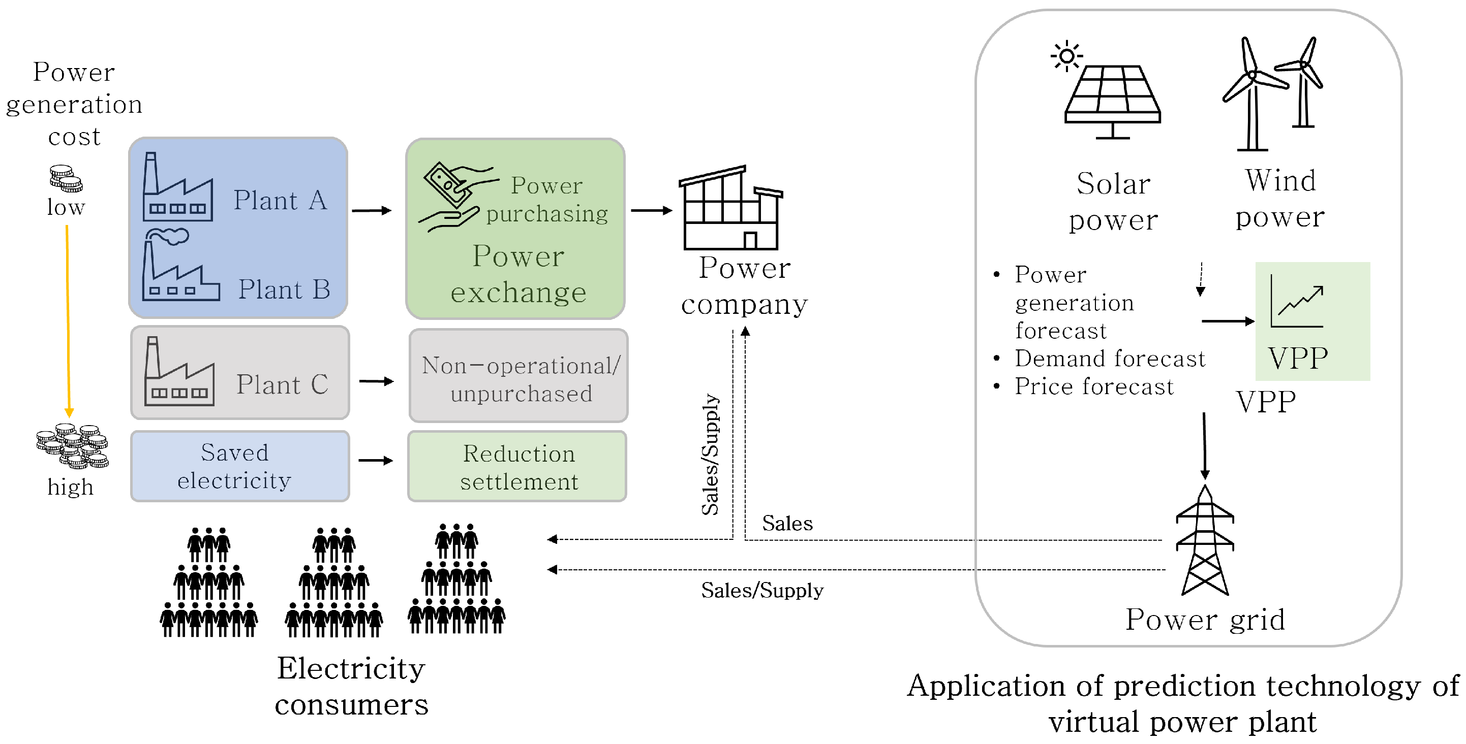
As shown in Figure 1, in the case of the currently produced electricity in Republic of Korea, it is collected by the network manager, Korea Electric Power Corporation, through the transmission network and then delivered to the user through the distribution network. Such a centralized management system is now changing to a distributed power generation system to compensate for the limitations in managing distributed power sources of various sizes distributed nationwide. The distributed power generation system supplies distributed resources to consumers by using small-scale power generation facilities in the vicinity of the consumers. However, when operating as such a distributed power source, each individual power source participates in the supply of electricity, and in this case, an error in the prediction of the amount of electricity generation increases, resulting in system operation problems. To solve this problem, the Korean government opened the power brokerage market in February 2019, and a Virtual Power Plant (VPP) that plays the role of brokerage transaction was created in this market.

Even if the VPP is operated, it does not fundamentally solve the problem of forecasting electricity generation from wind power. Forecasting wind power generation is crucial because inaccurate predictions of wind power generation result in unstable electricity supplies. The uncertainty on the electricity supply gives rise to the inaccurate plan of electricity supply. This could result in a blackout, which happens when demand exceeds supply. Additionally, it can result in an oversupply if there is little demand and lots of supply. In the latter scenario, the quality of the electricity degrades when an excess power supply occurs because it deviates from the conventional electric frequency (e.g., 60 ± 0.5 Hz in Republic of Korea). In particular, this overstock issue has a significant impact on the advanced precision industry, such as semiconductors with nano-scale circuits.

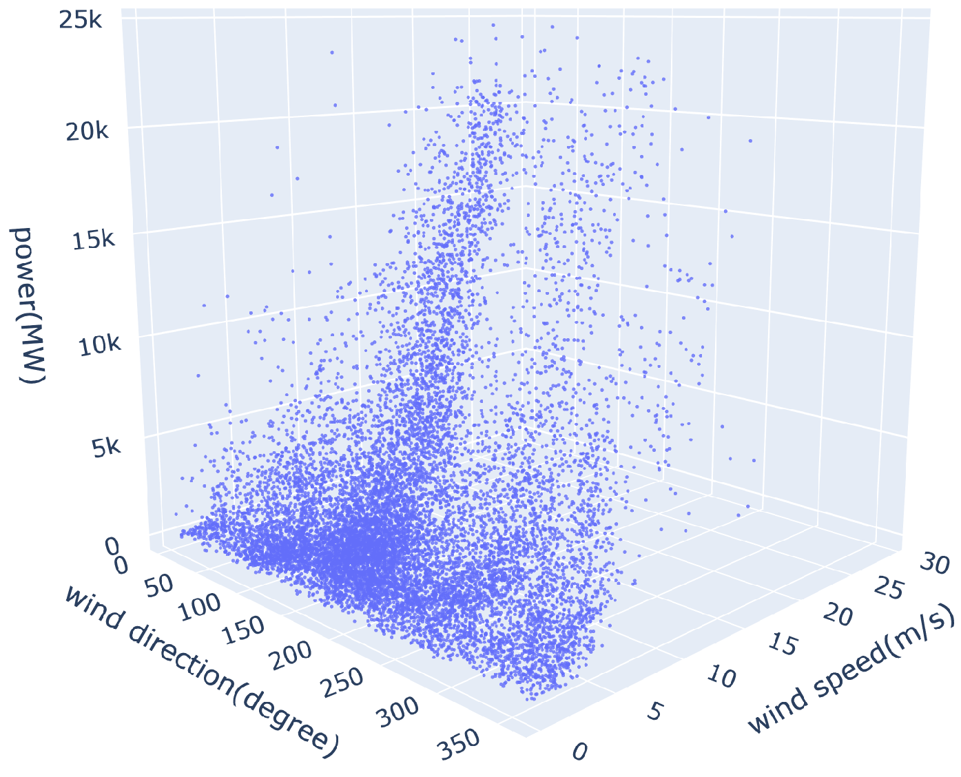
In general, wind power refers to a power generation method that uses wind energy to produce electricity, and it operates on the principle of converting mechanical energy generated by rotating blades into electrical energy through a generator. Since the output of the wind turbine is greatly affected by the wind speed, it is not easy to generate the desired amount of electricity at the desired time. The output characteristics of the wind power generator are divided into three main categories: the starting point wind speed at which the wind power generator starts producing output, the rated output wind speed at which the rated output occurs, and the wind speed at the output end point at which power is no longer generated for device protection while maintaining the rating.

1.2. Purpose of This Study

Solar power based on solar radiation can be predicted relatively reliably, but in the case of wind power generation, generated power varies rapidly due to the fluctuation of various factors such as weather and location, as well as wind speed and direction, which do not have a uniform pattern. It is also dependent on terrain, humidity, date and time of the day [1]. Thus, it is difficult to predict the wind power generation and is highly likely to cause power system instability, which brings great difficulty in stable system operation. Moreover, since the number of new wind power generators has rapidly increased in recent years, it is essential to accurately predict the amount of power generation of these new generators for stable and efficient wind power system linkages and system operations.

Wind Power Forecasting (shortly called WPF) involves a physical approach that builds sophisticated numerical models, analyzes and predicts the correlations between wind power and related variables, and a data-driven approach based on a vast amount of historical data. In this study, we deal with a mid-term wind power forecasting problem. The electricity market is largely divided into a day exhibition market, a real-time market, and an auxiliary service market. In this study, we developed an algorithm that predicts power generation one day ahead in line with the day-ahead market currently being implemented in the Korean market. For one-day-ahead forecasting, we intend to use a data-driven approach that can effectively analyze nonlinear data such as wind power output, weather data, etc. This is due to the fact that, in addition to wind speed and other observable physical features, it is also required to take into account numerous climatic conditions, and the data-driven approach can foresee these various properties. In this study, we try to develop a deep learning model based on actual weather forecast data and historical data on wind power generation and then use transfer learning to predict the quantity of wind power generation from a new generator with less data.

In order to properly demonstrate the performance of a data-driven approach, an important factor is securing sufficient training data. However, it takes a lot of time or an excessive cost to obtain data, and in most cases, it is difficult to obtain sufficient data for an experiment in a short period of time. In this case, it is difficult to apply a data-driven approach. However, this problem can be overcome through the concept of transfer learning, in which the content learned in a specific field is reused in a new field. Because transfer learning does not require training a neural network model from the beginning thanks to knowledge transfer, the basic performance can be improved, and the model development and learning time are improved to bring improved final performance even when data are insufficient. It can be used effectively in any situation. Transfer learning using pre-learning results has been mainly used in image classification problems, but recently, it is also widely used in linear regression. The advantage of transfer learning is that it can solve the problem of wind power generation forecasting, in which a lot of new wind power generators are being generated, but the prediction accuracy is low due to the lack of data.

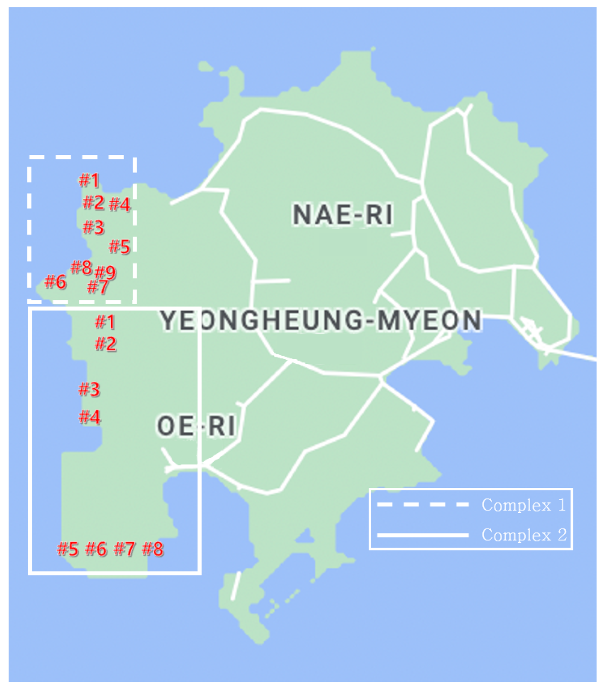
In this study, the effectiveness of the proposed transfer learning approach will be verified for wind power generators installed in two wind power complexes. After learning the power generation data of a wind power generator in a wind power complex where data have been accumulated for a relatively long period of time using the transfer learning approach, we apply it to predicting the mid-term (one day ahead) power generation amount of a wind power generator in a new wind power complex where the generation data are insufficient shortly after it was built.

2. Previous Works

So far, a number of studies have been conducted in relation to WPF. There have been some review works on WPF. For example, Monteiro et al. (2009) [2] have reviewed and analyzed detailed WPF approaches and their applications to power system operations. Hanifi et al. (2020) [1] systematically reviewed the state-of-the-art approaches of WPF with regard to physical, statistical (time series and artificial neural networks) and hybrid methods, including factors that affect accuracy and computational time in the predictive modeling efforts. Maldonado-Correa et al. (2021) [3] reviewed the predictive models of wind energy, aiming to establish the baseline for the development of a short-term wind energy prediction model that employs artificial intelligence tools.

Hu et al. (2016) [4] classified the WPF research methods into four categories: (i) physical models, (ii) conventional statistical models, (iii) spatial correlation models, and (iv) artificial intelligence and new models. Broadly classifying them, they can be divided into physics-based, statistics, and data-driven approaches. Physical methods use detailed physical characterization to model wind turbines/farms. This modeling effort was often carried out by down-scaling the Numerical Weather Prediction (NWP) data, which requires a description of the area, such as roughness and obstacles, as well as weather forecasting data of temperature, pressure, etc. [1]. Even though this method is perhaps the best choice for medium to long-term wind power prediction, it is computationally complex and, therefore, needs considerable computing resources [1,5].

Some previous works applied a statistical approach to WPF. For example, Choy et al. (2016) [6] derived a regression equation using wind speed and output data of the Jeju wind farm and predicted wind power generation. As a result of the regression analysis, it was shown that there was a high correlation between the predicted result and the actual output. Fang and Chiang (2016) [7] proposed a forecasting model consisting of the Gaussian process with a novel composite covariance function for high-accuracy wind power forecasting. They showed the effectiveness of the proposed model for the 2012 global energy forecasting competition wind power forecasting data. Furthermore, Chen (2018) [8] compared conventional (Autoregressive Moving Average (ARMA)) and two artificial intelligence methods (Artificial Neural Networks (ANNs) and Adaptive Neuro-fuzzy Inference Systems (ANFIS)) for wind power forecasting. In their experiments, they showed that ANNs and ANFIS were suitable for the very short-term (10 min ahead) wind speed and power forecasting, and the ARMA was suitable for the short-term (1 h ahead) wind speed and power forecasting.

Recently, many studies have been conducted in relation to WPF using a data-driven approach. For example, Park and Kim (2016) [9] compared the neural network model with the time series model and suggested a better model. Wind speed and wind direction data were used for model fit, and the neural network model and time series model were evaluated using the Mean Absolute Error (MAE). As a result, the ARMA-GARCH or ARMAX model performed better for predictions 1–3 h before, and the neural network model performed better for predictions after 6 h. Kim et al. (2017) [10] proposed a WPF method that reflects wind characteristics to improve the accuracy of wind power generation prediction. To extract the wind characteristics, correlation analysis of power generation, wind direction and wind speed was used. Based on the correlation, K-means clustering was performed to extract feature vectors. In addition, machine learning was performed using Support Vector Regression (SVR) to predict wind power generation. Root Mean Square Error (RMSE) was used as a performance evaluation index. Furthermore, Eissa et al. (2018) [11] devised a hybrid model for wind power forecasting through analytical data, multiple linear regressions and least square methods. ARMA, SVM, and ANN were used to verify the devised model, and it was concluded that the prediction accuracy using the hybrid model is generally superior to the accuracy using the individual model. Tian et al. (2018) [12] proposed a short-term wind power prediction method based on Empirical Mode Decomposition (EMD) and Extreme Learning Machine (ELM) for accurate wind power prediction. Through EMD, the wind power time series was decomposed based on fluctuations or trends of different scales, and an ELM model was built according to the characteristics of each component. Zhang et al. (2019) [5] used a deep learning network to forecast the wind turbine power based on a Long Short-Term Memory network (LSTM) algorithm and used the Gaussian Mixture Model (GMM) to analyze the error distribution characteristics of short-term WPF.

In addition, Lee et al. (2020) [13] implemented a model for predicting the output of a wind power complex which is located at Jeju island in Republic of Korea. In their model, an LSTM model, a type of Recurrent Neural Network (RNN) model, was used for 8 months of data. RMSE and Mean Absolute Percentage Error (MAPE) were used to determine the accuracy of the implemented model. As a result of the study, it was confirmed that the LSTM model has higher accuracy than the ANN and SVR models. Yang et al. (2021) [14] proposed an improved Fuzzy C-means (FCM) clustering algorithm to increase the accuracy of prediction results and reduce the complexity of the model. The FCM method classifies wind turbines with similar output characteristics into several categories and predicts the amount of power generation by applying the power curve representing each category. Dong et al. (2021) [15] proposed an ensemble learning model based on the stacking framework for WPF. In their model, first, an optimal decomposition method was selected to preprocess the wind data source, and second, a quadratic interpolation method based on state transition algorithm was proposed to optimize the parameters of the polynomial model and the weights of the neural network. Finally, a two-layer stack ensemble model was proposed. Experimental results showed that the proposed model has higher prediction accuracy and stability than other single prediction models. Wang and Wang (2021) [16] proposed an ensemble model of Multi-Layer Perceptron (MLP) to prevent overfitting and reduce the variance of a single MLP model. To predict solar power generation, k-MLP models were created by clustering days with similar power generation patterns, and predicted values were calculated by weighting k models. The proposed ensemble method performed better than a single MLP model.

There were also transfer learning approaches for WPF. For example, Hu et al. (2016) [4] proposed a deep learning approach using a transfer learning strategy for wind speed prediction. In their work, for transfer learning, they used a shared-hidden-layer deep neural network (DNN) architecture in which the hidden layers are shared across the domains and the output layers are different in each domain. They showed that the proposed architecture is highly beneficial for a wind farm with insufficient training data. Qureshi et al. (2017) [17] proposed a DNN model using transfer learning and ensemble techniques. A deep auto-encoder acts as a base-regressor, and a Deep Belief Network (DBN) is used as a meta-regressor. Furthermore, Cao et al. (2018) [18] proposed a transfer learning strategy for short-term WPF. They applied a nearest-neighbors approach to select highly relevant historical data from other wind farms. In order to enrich the training dataset, the K-Nearest Neighbors (KNN) algorithm is applied to select data from the other wind farm. Based on the new training dataset, four data-mining algorithms, Jaya-XGBoost, SVM, Least Absolute Shrinkage and Selection Operator (LASSO) and neural networks, were utilized to develop the wind forecasting model with different time horizons. In addition, Qureshi and Khan (2019) [19] proposed Adaptive Transfer Learning (ATL-DNN) for WPF. Using transfer learning, it was confirmed that the model learned from other wind farms can be applied, and ATL-DNN not only helps to provide weight initialization but also helps to provide an effective learning method. Deng et al. (2020) [20] looked into how deep learning, reinforcement learning and transfer learning are applied in wind speed and wind power forecasting, especially in the areas of data processing of wind power, input features selection, forecasting model framework establishment and model structure optimization. They compared deep-learning-related approaches including feed-forward network and RNN, and determined their strengths and applicability in the context of wind modeling methods. Luo et al. (2022) [21] used the KNN algorithm to form clusters according to the generation pattern and proposed a model combining separate transfer learning and LSTM algorithms (C-LSTM) for each cluster. They claimed that the performance of the model combining transfer learning and the LSTM model was improved by up to 68.4% compared to the standard LSTM model.

Table 1. Previous WPF works (data driven and transfer learning approaches).

Approach	Previous Works	Subject
Data-driven	Choy et al. (2016) [6]	- prediction of wind power generation with based regression analysis based on the Jeju wind farm
	Park and Kim (2016) [9]	- comparing the neural network model and the time series model
	Kim et al. (2017) [10]	- SVR for predicting wind power generation that reflects the characteristics of wind
	Eissa et al. (2018) [11]	- hybrid model for wind power forecasting through analytical data, multiple linear regressions and least square methods
	Tian et al. (2018) [12]	- wind power prediction method based on EMD and ELM for accurate wind power prediction
	Zhang et al. (2019) [5]	- deep learning network to forecast the wind turbine power based on an LSTM algorithm and used the GMM
	Lee et al. (2020) [13] Dong et al. (2021) [15]	- LSTM for the wind power farm at Jeju island
	Dong et al. (2021) [15]	- various decomposition techniques, parameter optimization, and stacking ensemble models for wind power predictive models
	Yang et al. (2021) [14]	- improved FCM clustering algorithm to increase the accuracy of prediction results
Transfer-learning	Hu et al. (2016) [4]	- shared-hidden-layer deep neural network (DNN)-based transfer learning approach
	Qureshi et al. (2017) [17]	- DNN model using transfer learning and ensemble techniques
	Cao et al. (2018) [18]	- KNN, Jaya-XGBoost, SVM, LASSO and neural networks short term wind power forecasting
	Qureshi and Khan (2019) [19]	- Adaptive Transfer Learning (ATL-DNN) for wind power generation prediction.
	Deng et al. (2020) [20]	- deep learning, enforcement learning and transfer learning are applied in wind speed and wind power forecasting
	Luo et al. (2022) [21]	- combining separate transfer learning and LSTM for each cluster classified by KNN

briefly summarizes the previous works related to a data-driven approach and transfer learning approach.

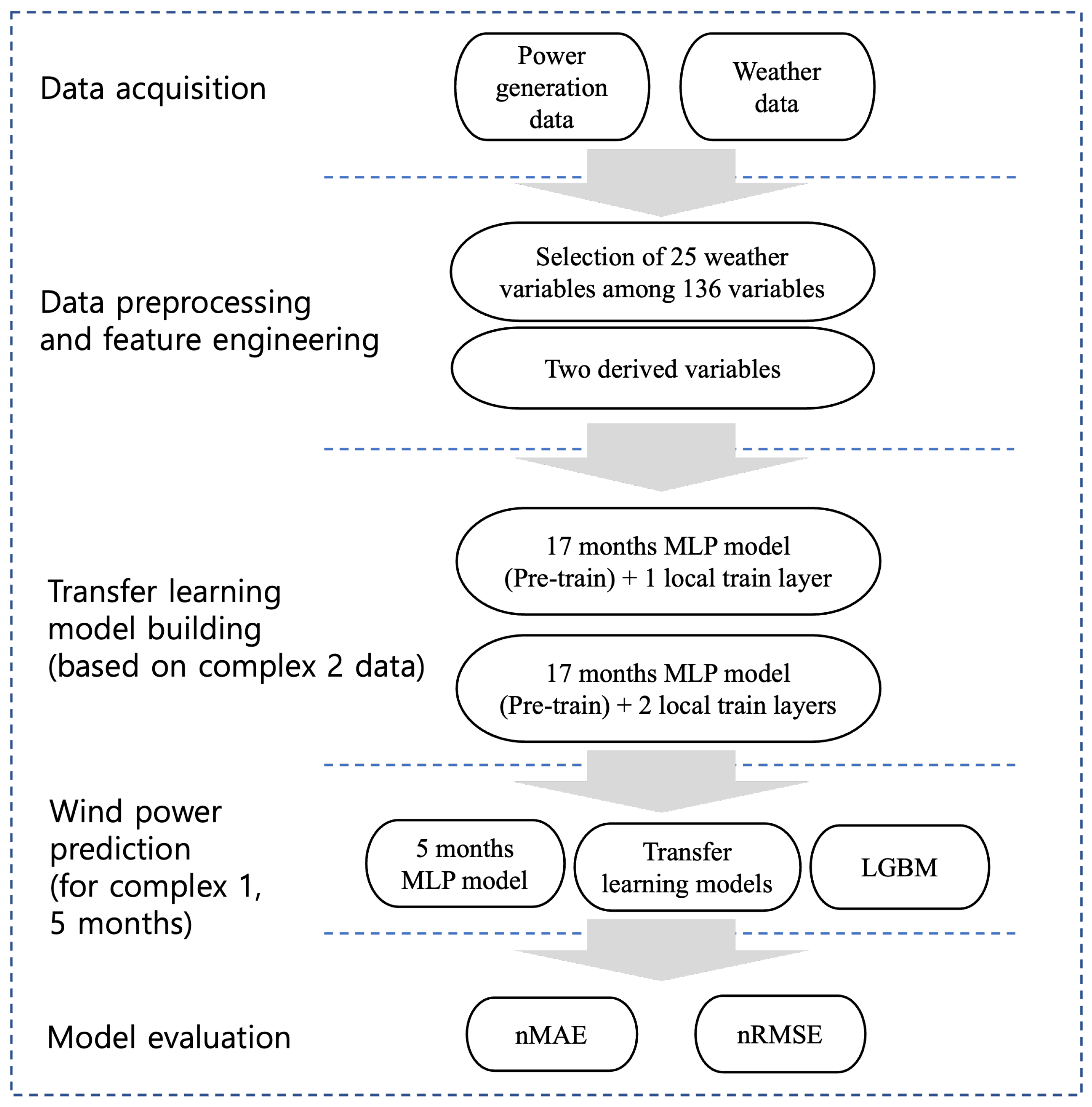
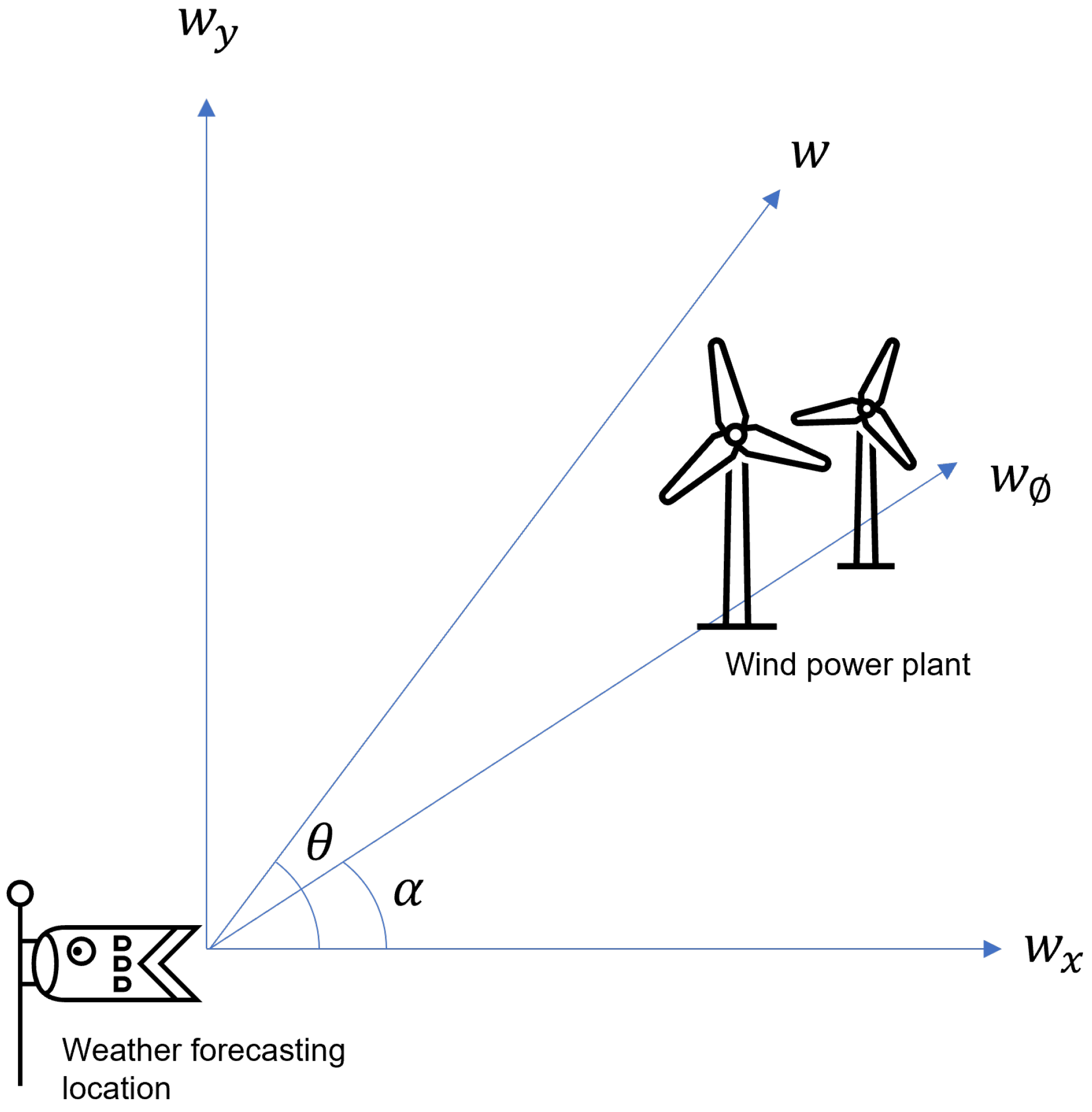
Although there has been quite a few data-driven approaches or transfer-learning-related studies on WPF problems so far, the differences between this study and previous studies related to data-driven approaches and transfer learning are as follows. First, WPF algorithms based on deep learning among previous data-driven approaches basically require a lot of data. However, these algorithms are not suitable for the problem of predicting the generation amount of a wind power plant with little operational data. As reviewed in previous studies, to overcome these problems, many transfer learning methods have been proposed for wind power generation forecasting, and they have been particularly used for short-term forecasting problems. However, this study focuses on the mid-term forecasting problem. Furthermore, in this study, in order to predict the amount of wind power generation more precisely, not only the existing weather observation data but also two derived variables were additionally considered and used for prediction. One of the derived variables is a variable that calculates the estimated wind speed value at the actual location of the wind power generator, not the wind speed data at the meteorological observation location, and the other derived variable is a variable related to the wind speed time point data considering the correlation with the wind power generation. This can also be said to be a differentiating point from previous transfer learning approaches. Finally, in deep learning or transfer learning, there are many research cases based on user experience or intuition for hyperparameter optimization, but in this study, grid search was used for hyperparameter optimization required for transfer learning.

In summary, the contributions of this study are summarized as follows. In this study, a case study was conducted in which the transfer learning technique was applied to the mid-term wind power generation prediction problem of a wind farm in Korea. Although the wind power generation prediction method applying the transfer learning method has been used in several previous studies, it is meaningful in that it verified the usefulness of the transfer learning method for wind power generation prediction based on the actual operation data of wind farms and the electricity market situation in Korea. In particular, as a result of the verification experiment, it was found that the deep-learning-based transfer learning method showed better performance in predicting the mid-term wind power generation of a newly completed wind power generator than a simple machine learning algorithm.

3. Approach

3.1. Transfer Learning

Transfer learning is a learning technique in which a model trained in a field with large data is reused in another field to improve the performance of a task with small data. Transfer learning is used to alleviate the data shortage issue for newly introduced system learning and to accelerate model training. This is achievable since the transfer learning strategy initially boosts quicker learning. In comparison to applying randomly initialized weights, the transfer learning strategy converges to a better degree of learning outcomes. Thanks to these advantages, the transfer learning is actively used in various industries such as image processing, voice recognition, and natural language processing.

In transfer learning, when a pre-trained neural network model is used, the hidden layer containing the contents of existing learning is reused. At this time, it is important to determine how many hidden layers are to be reused. In general, the reuse of the lower hidden layer close to the input layer is first reviewed, and the range of the reused hidden layer is sequentially expanded and, finally, the higher hidden layer close to the output layer. The reason for reviewing the reuse/use of the hidden layer close to the input layer in the first place is because this hidden layer processes information of an abstract nature inherent in the data. On the other hand, it is known that the closer the hidden layer is to the output layer, the more specific information that can be applied to a specific field is processed.

In this study, since the experiment was conducted on the assumption that the dataset size to be solved is small and similar to the previously learned dataset, the transfer learning model proceeded in the direction of reusing most of the hidden layers.

3.2. Input Variables

3.2.1. Data for Wind Power Forecasting

To evaluate the effectiveness of the proposed approach, the wind power generation data of the Yeongheung wind power complex located in Yeongheung-do, the west side area of South Korea, was used (refer to Figure 2). Yeongheung wind power complex 1 is composed of 9 units (total installed capacity of 22 megawatts and 8 units (total installed capacity of 24 megawatts) in complex 2 (total installed capacity of 24 megawatts). Complex 1 is all located in the west, and complex 2 has 4 units in the west and 4 units in the south. For the experiment, hourly power generation data (1 October 2019∼20 February 2021) for 17 months was obtained from the Republic of Korea public data portal (www.data.go.kr, accessed on 6 December 2022). Among the data, data without numerical values were deleted, and data for the period when a fire occurred or the generator was stopped due to the influence of wind in the complex were also excluded. As a result, this study used about 3360 data for about 5 months (1 October 2019∼20 February 2021) collected from Yeongheung wind power complex 1, and about 12,144 data collected from Yeongheung wind power complex 2 for about 1 year and 5 months (1 October 2019∼20 February 2021). In this study, we will make a transfer learning model pre-learning the data related to wind power generation accumulated over 17 months in complex 2 and then apply it to the prediction of the generation amount of the new wind power generator in complex 1. For the validation of the proposed transfer learning approach, we will use the power generation data for 5 months of the wind power generator in complex 1.

3.2.2. Weather Variables

For weather variables, the local forecast model (LDAPS, Local Data Assimilation and Prediction System) fileset provided by the meteorological data open portal of the Republic of Korea meteorological administration was used. The local forecast model has a spatial resolution of 1.5 km and is composed of 70 layers up to about 40 km vertically, and the prediction is performed 4 times a day (00:00, 06:00, 12:00, 18:00 UTC) by receiving the boundary field from the global model. The weather forecast data used in this study utilized the UK Meteorological Office’s operational model, the unified model (UM). UM receives boundary fields from the global model at 3 h intervals and performs predictions 8 times a day (00, 06, 12, 18UTC: 48-h prediction, 03, 09, 15, 21UTC: 3-h prediction). Since this study deals with day-ahead prediction, data predicted up to 48-h later was used. Two types of output data of the local forecasting model are provided: single-sided data and isostatic surface data. In this study, single-sided data were used. The single-sided forecast data provides a total of 136 variables. In this study, throughout feature engineering, 25 input variables closely related to wind power generation, as shown in

Table 2. Input variables.

Feature Abbreviation	Description	Unit	Range	γ*
NDNSW	Net Down Surface Shortwave Flux	W/m2	0.00∼1034.28	0.23
NCPCP	Large-Scale Precipitation (non-convective)	kg/m2	0.00∼144.52	0.1
SNOL	Large-scale Snow	kg/m2	0.00∼0.80	0.044
UGRD	U-Component of Wind at 10 m above ground	m/s	−23.23∼28.80	0.57
VGRD	V-Component of Wind at 10 m above ground	m/s	−34.70∼23.74	−0.57
TMP1.5	Temperature at 1.5 m above ground	K	271.62∼305.00	−0.46
TMIN	Minimum Temperature	K	271.39∼304.31	−0.5
TMAX	Maximum Temperature	K	272.14∼305.06	−0.5
SPFH	Specific Humidity at 1.5 m above ground	kg/kg	0.00∼0.02	−0.67
RH	Relative Humidity at 1.5 m above ground	%	29.18∼101.43	−0.65
VIS	Visibility at 1.5 m above ground	m	51.21∼94,286.45	0.64
DPT	Dew point Temperature	K	268.24∼300.23	−0.53
MXGUST	Maximum Wind Speed at 0 m above ground	m/s	0.75∼57.06	0.83
LCDC	Low Cloud Cover	%	0.00∼1.00	−0.09
MCDC	Medium Cloud Cover	%	0.00∼1.00	−0.15
HCDC	High Cloud Cover	%	0.00∼1.00	−0.4
TCAR	Total Cloud Amount Random Overlap	%	0.00∼1.00	−0.4
PRMSL	Pressure Reduced to Mean Sea Level	Pa	96395.60∼103,564.93	−0.3
TMP	Temperature	K	286.14∼301.75	−0.4
PRES	Pressure	Pa	96396.03∼103,564.96	−0.31
N50MU	50 m Wind U-Component	m/s	−25.89∼35.73	0.6
N50MV	50 m Wind V-Component	m/s	−38.88∼28.09	−0.58
SWDIR	Direct Shortwave Flux	W/m2	0.00∼972.05	−0.15
SWDIF	Diffuse Shortwave Radiation Flux	W/m2	0.00∼517.70	−0.42
TDSWS	Total Downward Surface Shortwave Flux	W/m2	0.00∼1070.57	0.19

^*γ: Pearson correlation coefficient.

, were selected and used in the model.

3.3. Overview of the Proposed Approach

In this study, after pre-learning 17 months of data from Yeongheung wind power complex 2, we will examine the performance of the transfer learning approach model for predicting the generation amount of Yeongheung wind power complex 1, which has relatively little data (5 months). To this end, the approach as shown in Figure 3 is as follows: First, with the wind power generation data and weather forecast data obtained from the Republic of Korea public data portal (www.data.go.kr, accessed on 6 December 2022), data preprocessing was carried out. In this study, min-max scaling, removal of missing values, removal of outliers, addition of derived variables, and data reduction through feature selection were performed for data preprocessing. Furthermore, in order to know the actual amount of power generated by the wind turbine, the amount of power generation by time period was separately calculated. In this study, variables that are judged to be somewhat related to the amount of power generation among a total of 136 weather forecasting variables were narrowed down through correlation analysis and qualitative judgment. Variables with high quantitative correlation coefficient values but also variables related to some basic weather variables such as NCPCP, SNOL, LCDC, and so on, even if the correlation coefficient values were low, were selected because other variables of more than 100 types, such as friction velocity, ICAO height of convective cloud base, and fog fraction, are judged to be difficult to affect wind power generation or can be replaced with these basic variables, and as shown in Table 2, finally 25 variables were selected and used in our model. In addition, in this study, to predict the one-day-ahead wind power generation in a more accurate manner, two variables were additionally derived and used in our model: (1) wind speed variable for predicting wind speed at the location of the wind power generator rather than at the meteorological observation point and (2) wind-speed-derived variable considering the correlation with power generation. Then, a transfer learning model was created to predict complex 1 data by adding one and two local train layers, respectively, to the pre-trained MLP model using data from complex 2 with 17 months of data. The performance of the transfer learning approach was evaluated by comparing with the MLP-trained model without transfer learning and the Light Gradient Boosting Machine (LGBM) model with 5 months of data in complex 1. For evaluation, MAE and RMSE indicators were used. In this study, we have developed a one-day-ahead forecasting model that predicts the amount of power generation from 00:00 to 24:00 the next day with the weather numerical model data obtained around 14:00 the day before. The overall approach for our study is depicted in Figure 3.

3.4. Exploratory Data Analysis

3.4.1. Wind Speed Distribution and Wind Power Generation Distribution

Figure 4 shows the distribution of wind speed forecast data for 17 months at Yeongheung wind power complex 2. In fact, the distribution of the wind speed forecast data of the Yeongheung wind power complex 2 ranges from 0 to 30 m/s, but the wind speed exceeding 23 m/s appears very rarely, so it was judged to be an outlier and excluded from Figure 4. Considering that the minimum wind speed (start-up wind speed) at which the wind power generator starts generating electricity is 3 m/s, it can be seen that the wind speeds blowing in the Yeongheung wind complex are sufficient to generate electricity. The blades of the Yeongheung wind power generators are mainly directed to the west coast, and this is due to the fact that the yawing system senses the wind direction and rotates it around the vertical axis according to the geographical characteristics of Republic of Korea that are affected by the northwest monsoon wind. In Republic of Korea, it is known that the proportion of northwest winds is high in winter (December to February), and the proportion of southwest winds, such as southwest and southeast winds, is high in summer (June to August). Figure 5 shows the size of the amount of power produced by wind direction. Here, M in 2 M, 4 M,⋯, 10 M on the horizontal axis means megawatts. In Figure 5, the wind speed predicted in Yeongheung wind power complex 2 is distributed in the range of 0 to 30 m/s, which is divided into 2 m/s units. There were 545 time slots where wind speeds of 14 m/s or higher were forecasted, and they were merged into one category as there were fewer than 717 times when wind speeds were predicted to be between 12 and 14 m/s (717 times). A closer look at Figure 5 shows that the main wind direction of the Yeongheung wind power generators is the northwest wind, and the wind direction and wind speed with the largest amount of power generation were confirmed to be the northwest wind direction (NW) and 10 to 12 m/s speed, respectively.

3.4.2. Power Generation According to Wind Speed and Direction

In the previous section, we could see that the northwest wind (NW) showed the highest power generation efficiency. Figure 6 shows the wind direction, wind speed, and power generation by drawing a scatter plot in a three-dimensional space. A relatively large amount of power generation is distributed near 135 degrees (NW), and many points close to the 24 megawatts rated output of Yeongheung wind power complex 2 are observed. The most observed wind direction after the northwest wind series is the southwest wind series around 235 degrees, showing a similar shape to the northwest wind series, although it is less frequent. In the northwest wind series and the southwest wind series, the wind power generator power curve is relatively shown, but it does not converge to the output curve in the other wind directions.

3.5. Preprocessing of Input Variables

3.5.1. Wind Speed Derived Variable Considering Effective Wind Direction

In this study, to understand how wind speed forecasting data actually affected the amount of wind power generation, we estimated the wind speed at the generator location ($W_{\varphi }$) based on east–west wind speed and north–south wind speed at the weather forecast location (refer to Figure 7). The closest meteorological observation point to the Yeongheung wind power complex is about 4 to 5 km away from each wind power generator, and the angle between the meteorological observation point and the wind power complex is also distributed over a wide range. The wind speed data provided by the LDAPS meteorological model includes east–west wind speed (u) and north–south wind speed (v). From the u and v wind speeds, according to ECMWF [22], the wind direction ($\theta$) can be obtained as follows.

$$\theta =mod(180+\frac{180}{\pi }atan2(v,u),360)$$

(1)

Analyzing results showed that the wind direction parameter ($\alpha$) had the highest correlation with power generation when the parameter was 40°, 45°, and 50°, respectively. Hence, in this study, it is assumed that the weather observation point and the representative generator of Yeongheung wind power complex 1 are located at a 45° angle, i.e., $\alpha =45°$.

As a result, $W_{\varphi }$ (estimated wind speed variable) could be calculated by the following Equation (3) (when $\alpha =45°$).

$$W_x=W·cos\theta ,W_y=W·sin\theta$$

(2)

$$\begin{array}{cc}\hfill W_{\varphi }=& W·cos(\theta -\alpha )\hfill \end{array}$$

(3)

$$\begin{array}{cc}\hfill =& W·cos\theta cos\alpha +W·sin\theta sin\alpha \hfill \end{array}$$

(4)

$$\begin{array}{cc}\hfill =& W_x·cos\alpha +W_y·sin\alpha \hfill \end{array}$$

(5)

In this study, as shown in

Table 3. Pearson’s correlation coefficient with power generation at various angles.

Angle	10°	20°	30°	40°	45°	50°	60°	70°	80°	90°
Power generation	0.63	0.67	0.7	0.72	0.72	0.72	0.71	0.69	0.65	0.6

, the Pearson correlation coefficient with power generation was calculated by adding wind speeds at various angles to obtain the appropriate wind direction ($\alpha$) for the Yeongheung wind power complex. Looking at the correlation with the amount of power generation, it can be seen that when the wind direction ($\alpha$) is 40°, 45°, and 50°, it is 0.72, which has the highest correlation. This means that the angle between Yeongheung wind power complex 1 and the meteorological observation point has a value between 40° and 50°. As a result, in this study, it is assumed that the weather observation point and the representative generator of Yeongheung wind power complex 1 are located at a 45° angle.

3.5.2. Wind Speed Derived Variable Considering Correlation with Power Generation

The wind power generation data of the Yeongheung wind power complexes provided by the public data portal are accumulated values over time. However, in the case of meteorological data, there is a problem in that an appropriate forecast value needs to be mapped when mapping it with the power generation data because it provides a forecast value of an instantaneous time point by time. As shown in Figure 8, if there is a difference between the predicted wind speed at time t and the predicted wind speed at time $t+1$, it is necessary to check the wind speed prediction time point, which has a higher correlation with the accumulated power generation value at time t. In addition, in the case of wind speed data, a negative value exists because direction information is included. Therefore, the correlation with the amount of power generation was checked by adding the absolute values of the east–west wind speed (U-Component) and the north–south direction wind speed (V-Component).

As the results of correlation analysis (refer to

Table 4. Pearson’s correlation coefficient with power generation by time point.

Variable	U_pre	V_pre	U_post	V_post	U_abs_pre	V_abs_pre	U_abs_post	V_abs_post	45_pre	45_post
Power generation	0.43	−0.13	0.43	−0.15	0.56	0.6	0.57	0.6	0.72	0.73

), in all variables, the variable at time $t+1$ (noted as post in the variable name) showed a slightly higher correlation with the amount of power generation than the variable at time t (noted as pre in the variable name). Furthermore, variables that take absolute values of wind speed variables (U_abs_pre, V_abs_pre, U_abs_post, V_abs_post) seem to have a relatively high correlation coefficient with power generation compared to unprocessed wind speed variables (U_pre, V_pre, U_post, V_post). In addition, in the case of effective wind speed, it was observed that the correlation coefficient (0.73) with the variable at time $t+1$ (45_post) was slightly higher than the correlation coefficient (0.72) between the variable at time t (45_pre) and the amount of generation. In this study, based on the above results, not only the raw wind speed variable but also the absolute value variable and the wind speed variable at time $t+1$ are included and used by mapping with the accumulated power generation amount at time t.

3.6. Model Configuration

In this study, MLP was used to construct a transfer learning model for predicting wind power generation. MLP is one such deep learning method, and it is an artificial neural network hierarchical structure in which one or more hidden layers exist between the input layer and the output layer [23,24]. The optimal model is constructed through a learning process that adapts the neuron’s connection strength between each layer to the optimal state. After the feed-forward process of taking the output value considering the weight to the input value of the previous layer as the input value of the next layer, the weight is calculated and updated while calculating the slope of the input value with respect to the output value through the back-propagation process. Factors that affect the performance of MLP include the number of hidden layers, the number of nodes in each layer, optimization algorithm, learning rate, and activation function. In our experiment, according to the transfer learning scenario, it was assumed that the period of the newly completed generator with insufficient data was 5 months of Yeongheung wind power complex 1, and the prior data for transfer learning was assumed to be 17 months of Yeongheung wind power complex 2. In order to construct an MLP model with the maximum performance in each period, an experiment was conducted to construct a model separately, and an optimal model was individually constructed. The optimal model was found by combining the number of hidden layers and the number of nodes in each layer in various ways through the grid search method. In this study, in all experiments, 80% of the train set was extracted in chronological order, and 20% of the test set was extracted from the latest date.

In general, it is known that prediction is possible with only one or two hidden layers in MLP, but in this study, to verify the effect on transfer learning based on the existing learning model, the number of hidden layers was configured up to five. To prevent overfitting, batchNormalization was applied before all activation functions, and a dropout of 20% was applied whenever the number of neurons was changed. In addition, as the nonlinear activation function, ReLU, which has the advantage of learning faster as the neural network deepens, is used to compensate for the disadvantages of activation functions, such as sigmoid and tanh, which show gradient vanishing as the gradient approaches to zero [23,25].

3.6.1. Deep Learning Model with 5 Months of Data

Assuming a new generator would be built, an experiment was carried out with 5-month data from Yeongheung wind power complex 1 to construct a model of a generator with insufficient data. All experiments were repeated 10 times, the average was calculated, and parameters were set through the grid search method among the hyperparameter optimization methods of AutoML. The reason why the experiment was repeated 10 times was as follows: In order to determine the optimal value of hyperparameters such as the number of nodes and layers in the proposed model, experiments were repeatedly conducted by changing the values of hyperparameters. However, even if the experiment was repeated more than 10 times, the performance index was similarly calculated, so it was limited to 10 times to minimize time complexity. As a result of the experiment (refer to

Table 5. Top 5 results of grid search by hidden layer configuration (5 months).

Node	nMAE (%)	Node	nMAE (%)	Node	nMAE (%)	Node	nMAE (%)	Node	nMAE (%)
500	11.03	64, 500	10.705	48, 256, 450	10.90	128, 128, 256, 350	11.00	24, 48, 450, 450, 450	11.02
550	11.04	100, 550	10.713	200, 256, 450	10.93	64, 200, 256, 450	11.03	48, 64, 200, 350, 500	11.03
400	11.07	48, 350	10.78	128, 350, 450	10.94	350, 350, 350, 500	11.05	256, 256, 450, 450, 450	11.05
256	11.10	12, 300	10.78	24, 400, 450	10.96	350, 350, 550, 550	11.08	350, 400, 450, 450, 450	11.06
300	11.13	256, 450	10.78	350, 350, 400	10.96	128, 256, 300, 400	11.09	128, 200, 500, 500, 500	11.09

), when the number of hidden layers was two and the number of nodes was 64 and 500, respectively, the performance was the best.

3.6.2. Deep Learning Model with 17 Months of Data

Assuming the existing generator, an experiment was conducted with 17 months of data from Yeongheung wind power complex 2 to construct a pre-training model for transfer learning. All experiments were conducted in the same manner as in the 5-month model configuration. As a result of the experiment (refer to

Table 6. Top 5 results of grid search by hidden layer configuration (17 months).

Node	nMAE (%)	Node	nMAE (%)	Node	nMAE (%)	Node	nMAE (%)	Node	nMAE (%)
550	9.56	550, 550	9.11	550, 550, 550	9.08	100, 300, 300, 300	9.05	400, 450, 450, 550, 550	9.15
350	9.60	400, 400	9.18	200, 400, 500	9.13	300, 300, 350, 400	9.08	200, 200, 300, 400, 400	9.15
256	9.62	400, 450	9.23	256, 400, 400	9.14	64, 64, 550, 550	9.13	100, 100, 200, 350, 350	9.17
300	9.63	500, 500	9.24	200, 500, 500	9.17	200, 256, 256, 400	9.16	200, 300, 450, 450, 450	9.17
500	9.63	300, 256	9.26	100, 350, 350	9.17	200, 450, 450, 500	9.17	256, 300, 300, 500, 550	9.19

), when the number of hidden layers was four and the number of nodes was 100, 300, 300, and 300, respectively, the performance was the best.

3.6.3. Transfer Learning Model Configuration

Figure 9 is a diagram of the transfer learning model. In this study, since the available dataset size for prediction is small and similar to the previously learned dataset, the transfer learning model proceeded in the direction of reusing most of the hidden layers. Furthermore, when creating a transfer learning model, we considered adding one or two layers to the existing pre-training model. It is assumed that the newly added layer has 300 nodes using ReLu as the activation function. In addition, in this study, learning_rate_scheduler was used as a callback function for the transfer learning model, and the initial learning rate of 0.01 was maintained until epoch 10. After that, when the learning rate was set to a value of 1/10 (i.e., 0.001) of the pre-learned model and the experiment was conducted, the performance was the best, so it was used as it is. Furthermore, Early_stopping_callback and learning_rate_scheduler were used as callback functions. The former is to prevent the accuracy of the training set increasing as learning progresses due to overfitting, but the experimental results of the test set gradually deteriorate. For this, the EarlyStopping function was used to stop learning when the test set error no longer decreased. In this experiment, it was set to wait up to 30 times even if the test error did not improve. The latter is a method of adjusting the learning rate in the learning process, and it is generally known that learning is better when the optimization is performed quickly with a large learning rate at first, and then the learning rate is reduced through fine adjustment as it approaches the optimal value. In this study, the learning rate set by the user was maintained until epoch 10, but the learning rate was set to decrease gradually after that.

3.7. Evaluation Metrics: nMAE and nRMSE

According to Maldonado-Correa et al. (2021) [3], RMSE and MAE are methods predominantly used for calculating errors in wind power forecast models. This study also used two metrics for comparing the performances of wind power forecast models. The followings show the details of MAE and RMSE.

3.7.1. MAE

In Equation (6), $O_i$ is the observed value, $P_i$ is the experimental value, and n is the number of samples. Thus, MAE means the average of the absolute error between the observed value and the predicted value. The best value is 0, and the higher the value, the worse the performance. Since MAE takes the absolute value of the error, the size of the error is reflected in the result value as it is. That is, it is a suitable indicator when the loss due to error increases linearly or when there are many outliers. In addition, since the error is expressed, the accuracy between wind power plants can be easily compared, and the disadvantages of RMSE that depend on the scale can be supplemented.

$$MAE=\frac{1}{n}\sum _{i=1}^n\left(\right|O_i-P_i\left|\right)$$

(6)

3.7.2. RMSE

RMSE means a value obtained by squaring the error between the observed value ($O_i$) and the predicted value ($P_i$) and averaging it, and it can be obtained as in Equation (7). As the value increases, it means that the prediction performance deteriorates. Since the error is squared, the larger the error, the higher the weight is reflected in proportion. It is a suitable indicator in a situation where the loss due to error increases exponentially. Furthermore, although it is a method to evaluate the accuracy of a representative predictive model, it has the disadvantage of being greatly affected by the scale.

$$RMSE=\sqrt{\frac{1}{n}\sum _{i=1}^n{(O_i-P_i)}^2}$$

(7)

Because the maximum power generation amount for each wind power plant was different, the size of the error between the plants was also different. Therefore, in order to compare the errors in the same unit, in this study, nominal Mean Absolute Error (nMAE) and nominal Root Mean Square Error (nRMSE) were used instead of MAE and RMSE, which were obtained by dividing the MAE and RMSE indicators by the installed capacity of each wind power plant (its maximum power generation). For the convenience of numerical comparison, nMAE (%) and nRMSE (%) obtained by multiplying the nMAE and nRMSE values by 100 were used.

4. Experimental Results

The experimental environment of this study was based on Python 3.9 and Tensorflow (deep learning open-source library). In this study, transfer learning of the pre-trained model in Yeongheung wind power complex 2 is carried out to improve the prediction of the performance of the Yeongheung wind power complex 1 because complex 1 is newly built, and there is very little historical data. To evaluate the performance of the proposed transfer learning approach, a model (called Model 1) using only data from Yeongheung wind power complex 1 in a new environment is compared with the transfer learning models that have been previously trained with data from Yeongheung wind power complex 2. In the case of the transfer learning models that were pre-training with data from Yeongheung Complex 2, they were divided into Model 2 and Model 3, which added one layer and two layers to the pre-training model, respectively. In addition, for performance comparison with machine learning, a model applied with LGBM, which is well-known for its speed and accuracy among tree-based learning algorithms, was additionally tested and the performance was compared. The following is a summary of the models used in the experiment for performance comparison.

• Model 1: simple MLP model only using data obtained from the new environment, i.e., Yeongheung wind power complex 1.
• Model 2: MLP-based transfer learning model that additionally added one layer into the pre-training model, which has learned the information of Yeongheung wind power complex 2 in advance.
• Model 3: MLP-based transfer learning model that additionally added two layers into the pre-training model, which has learned the information of Yeongheung wind power complex 2 in advance.
• LGBM: Light Gradient Boosting Machine.

The results of the models are shown in

Table 7. Experimental comparison results.

Models	nMAE (%)	nRMSE (%)	Accuracy (%)	Time (s)
Model 1	8.90	12.73	91.11	36.69
Model 2	7.87	11.26	92.22	12.61
Model 3	7.89	11.28	92.21	-
LGBM	8.29	11.31	91.71	-

. As the results of computational experiments, the nMAE and nRMSE of Model 1 without transfer learning were 8.90 and 12.73, and those of transfer learning models 2 and 3 were 7.87, 11.26, 7.89, and 11.28, respectively. Model 2 and Model 3 showed higher performance than Model 1 in both evaluation indicators, which seems to be because information learned in advance in a similar environment was used. Furthermore, looking at the results of LGBM, nMAE and nRMSE were 8.29 and 11.31, which showed better performance than the deep learning model without transfer learning (Model 1), but inferior in performance to Model 2 and Model 3 with transfer learning. Furthermore, it was discovered that the learning time was shortened by almost three times in the case of transfer learning. The performances of LGBM are better than those of Model 1, but inferior to transfer learning models. In general tabular data, the deep learning method is not often used well due to overfitting, but in this study, the deep-learning-based transfer learning approach showed better performance than LGBM. Comparing the performance of Model 2 and Model 3 to which the transfer learning approach is applied, it can be seen that the performance of Model 2, which is learned by adding only one layer to the pre-training model, is better.

In order to confirm the effect of transfer learning, a paired t-test was performed with the result index derived from 30 tests based on Model 1 and Model 2, as shown in

Table 8. Paired t-test result.

Metrics	Model	# of Samples	Avg.	Std.	t-Value	p-Value
nMAE	Model 1	30	7.81	1.08	2.42	0.01 **
nMAE	Model 2	30	7.59	1.23
nRMSE	Model 1	30	10.79	1.39	0.57	0.28 **
nRMSE	Model 2	30	10.71	1.51

** p < 0.05

. As a result, the paired t-test statistic of nMAE was calculated as 2.42, and the p-value was 0.01, confirming that there was a significant difference between Model 1 and Model 2 under the significance level of 5%. In terms of nRMSE, slightly different results were obtained compared to those of Table 7. The average nRMSE value of Model 2 was slightly small compared to that of Model 1, but the standard deviation of Model 2 was calculated to be slightly larger at 1.51, and it was difficult to see that there was a significant difference under the 5% significance level. Unlike the results in Table 7, the reason why the difference between Model 1 and Model 2 was not statistically significant in nRMSE because the data sets used in the experiment were different. That is, in the experiment in Table 7, the latest 20% of the data in Yeongheung Complex 1 was extracted and configured as a test-set, whereas in the experiment in Table 8, 20% of the data in Yeongheung Complex 1 was randomly extracted and the experiment was repeated 30 times. As a result of a more objective paired t-test, although there was no significant difference in the nRMSE index, the effect of transfer learning on the nMAE index appears to be statistically significant. For reference, since nMAE is selected as the performance indicator used in the power generation prediction system currently implemented by the Korean Power Exchange, it can be said that Model 2, with good performance of the nMAE indicator, is more meaningful in reality.

5. Conclusions

In this study, to develop an efficient wind power forecast model, a transfer learning model based on MLP was proposed. It was used to predict the power generation amount of the Yeongheungdo wind power generation complex 1, which is newly built and does not have many operational data. In the case of MLP, for the pre-training model with 17 months of data of complex 2, when the activation function was $ReLU$, with four hidden layers, and the number of nodes was 100, 300, 300, and 300, it showed the best performance. In the case of transfer learning, the best results were obtained from the model in which all four existing layers applied in the pre-training model were retrained, and then one additional layer was trained. Under these conditions, it was confirmed that the prediction performance was improved in predicting the power generation amount using transfer learning after learning the Yeongheung wind power complex 2 than when predicting the Yeongheung wind power complex 1 by MLP alone.

As the linkage of new and renewable energy sources to the existing power system increases, the importance of the system operation stabilization system increases. Accordingly, technology that can predict power supply and demand is becoming more important. Sufficient data are needed to train a predictive model that can predict power generation, but in reality, newly introduced systems have a limitation in that they lack initial data. To overcome this limitation, in this study, transfer learning was used to solve this problem, and transfer learning was applied to the prediction of wind power generation and showed better results than the method without transfer learning. As the result, it is expected that the prediction accuracy of a new wind power generator will be improved by using transfer learning, and it will be possible to reach the power system stabilization more quickly.

Despite this meaningful achievement, this study has some shortcomings in the following points, so it is necessary to consider them as future research issues. First, statistical and probabilistic analysis approaches are needed for more data and cases. For example, it is necessary to verify statistically whether wind speed/generation amount predictions of wind power complexes 1 and 2 can be statistically similar. Furthermore, in feature selection, a more statistical verification method is needed for the used correlation analysis part. Second, in this study, only relatively simple and well-known deep learning and machine learning models have been applied, but it is necessary to further verify the performance of transfer learning by applying other machine learning models and deep learning models. For example, we could consider a subject that increases the prediction accuracy by using a model such as Conv-LSTM, which combines CNN and LSTM, which is easy to predict time series data. Third, since the wind speed variable that has the greatest influence on the amount of wind power generation is the day-ahead forecast data, an error correction model for forecast variables should be preceded. However, in this study, there is a limitation that an error correction model could not be developed because the measured wind speed observed at the wind power plant site was missing. Finally, since the amount of electricity production shows different characteristics depending on the region, such as the input factors used according to the climate, season, and topography according to the wind power generation region, it is also necessary to take into account the improvement of the accuracy of wind power generation forecasting by reflecting it after analyzing the cause of the difference in the power generation according to the difference in the input factors by region.

References

1. Hanifi, S.; Liu, X.; Lin, Z.; Lotfian, S. A critical review of wind power forecasting methods—Past, present and future. Energies 2020, 13, 3764. [Google Scholar] [CrossRef]
2. Monteiro, C.; Bessa, R.; Miranda, V.; Botterud, A.; Wang, J.; Conzelmann, G. Wind Power Forecasting: State-of-the-Art 2009; Technical report; Argonne National Lab. (ANL): Argonne, IL, USA, 2009. [Google Scholar]
3. Maldonado-Correa, J.; Solano, J.; Rojas-Moncayo, M. Wind power forecasting: A systematic literature review. Wind Eng. 2021, 45, 413–426. [Google Scholar] [CrossRef]
4. Hu, Q.; Zhang, R.; Zhou, Y. Transfer learning for short-term wind speed prediction with deep neural networks. Renew. Energy 2016, 85, 83–95. [Google Scholar] [CrossRef]
5. Zhang, J.; Yan, J.; Infield, D.; Liu, Y.; Lien, F.S. Short-term forecasting and uncertainty analysis of wind turbine power based on long short-term memory network and Gaussian mixture model. Appl. Energy 2019, 241, 229–244. [Google Scholar] [CrossRef] [Green Version]
6. Choy, Y.; Jung, S.; Park, B.; Hur, J.; Park, S.; Yoon, G. Study on the Prediction of Wind Power Outputs using Curvilinear Regression. KEPCO J. Electr. Power Energy 2016, 2, 627–630. [Google Scholar] [CrossRef]
7. Fang, S.; Chiang, H.D. A high-accuracy wind power forecasting model. IEEE Trans. Power Syst. 2016, 32, 1589–1590. [Google Scholar] [CrossRef]
8. Chen, Q.; Folly, K. Wind power forecasting. IFAC-PapersOnLine 2018, 51, 414–419. [Google Scholar] [CrossRef]
9. Park, S.H.; Kim, S. A study on short-term wind power forecasting using time series models. Korean J. Appl. Stat. 2016, 29, 1373–1383. [Google Scholar]
10. Kim, Y.; Jeong, M.; Son, N. Forecasting of Short-term Wind Power Generation Based on SVR Using Characteristics of Wind Direction and Wind Speed. J. Korean Inst. Commun. Inf. Sci. 2017, 42, 1085–1092. [Google Scholar]
11. Eissa, M.; Yu, J.; Wang, S.; Liu, P. Assessment of wind power prediction using hybrid method and comparison with different models. J. Electr. Eng. Technol. 2018, 13, 1089–1098. [Google Scholar]
12. Tian, Z.; Ren, Y.; Wang, G. Short-term wind power prediction based on empirical mode decomposition and improved extreme learning machine. J. Electr. Eng. Technol. 2018, 13, 1841–1851. [Google Scholar]
13. Lee, H.; Kim, K.; Jeong, H.; Lee, H.; Kim, H.; Park, J. A Study on Wind Power Forecasting Using LSTM Method. Trans. Korean Inst. Electr. Eng. 2020, 69, 1157–1164. [Google Scholar] [CrossRef]
14. Yang, M.; Shi, C.; Liu, H. Day-ahead wind power forecasting based on the clustering of equivalent power curves. Energy 2021, 218, 119515. [Google Scholar] [CrossRef]
15. Dong, Y.; Zhang, H.; Wang, C.; Zhou, X. Wind power forecasting based on stacking ensemble model, decomposition and intelligent optimization algorithm. Neurocomputing 2021, 462, 169–184. [Google Scholar] [CrossRef]
16. Wang, M.; Wang, P. Ensemble Multilayer Perceptron Model for Day-ahead Photovoltaic Forecasting. In Proceedings of the 2021 4th International Conference on Control and Computer Vision, Macau, China, 13–15 August 2021; pp. 189–194. [Google Scholar]
17. Qureshi, A.S.; Khan, A.; Zameer, A.; Usman, A. Wind power prediction using deep neural network based meta regression and transfer learning. Appl. Soft Comput. 2017, 58, 742–755. [Google Scholar] [CrossRef]
18. Cao, L.; Wang, L.; Huang, C.; Luo, X.; Wang, J.H. A transfer learning strategy for short-term wind power forecasting. In Proceedings of the 2018 Chinese Automation Congress (CAC), Xi’an, China, 30 November–2 December 2018; IEEE: Piscataway, NJ, USA, 2018; pp. 3070–3075. [Google Scholar]
19. Qureshi, A.S.; Khan, A. Adaptive transfer learning in deep neural networks: Wind power prediction using knowledge transfer from region to region and between different task domains. Comput. Intell. 2019, 35, 1088–1112. [Google Scholar] [CrossRef] [Green Version]
20. Deng, X.; Shao, H.; Hu, C.; Jiang, D.; Jiang, Y. Wind power forecasting methods based on deep learning: A survey. Comput. Model. Eng. Sci. 2020, 122, 273. [Google Scholar] [CrossRef]
21. Luo, X.; Zhang, D.; Zhu, X. Combining transfer learning and constrained long short-term memory for power generation forecasting of newly-constructed photovoltaic plants. Renew. Energy 2022, 185, 1062–1077. [Google Scholar] [CrossRef]
22. European Centre for Medium-Range Weather Forecasts. ERA5: How to Calculate Wind Speed and Wind Direction from u and v Components of the Wind?; Technical report; ECMWF. Available online: https://confluence.ecmwf.int/pages/viewpage.action?pageId=133262398 (accessed on 6 December 2022).
23. Akpudo, U.E.; Hur, J.W. Intelligent solenoid pump fault detection based on MFCC features, LLE and SVM. In Proceedings of the 2020 International Conference on Artificial Intelligence in Information and Communication (ICAIIC), Fukuoka, Japan, 19–21 February 2020; IEEE: Piscataway, NJ, USA, 2020; pp. 404–408. [Google Scholar]
24. Montufar, G.F.; Pascanu, R.; Cho, K.; Bengio, Y. On the number of linear regions of deep neural networks. Adv. Neural Inf. Process. Syst. 2014, 27, 1–9. [Google Scholar]
25. Khalil Alsmadi, M.; Omar, K.B.; Noah, S.A.; Almarashdah, I. Performance comparison of multi-layer perceptron (Back Propagation, Delta Rule and Perceptron) algorithms in neural networks. In Proceedings of the 2009 IEEE International Advance Computing Conference, Patiala, India, 6–7 March 2009; IEEE: Piscataway, NJ, USA, 2009; pp. 296–299. [Google Scholar]
Figure 1. Electricity transaction flow chart in the Korean electricity market.
Electronics 11 04125 g001
Figure 2. Map on Yeongheung wind power complex (# indicates each wind power generator).
Electronics 11 04125 g002
Figure 3. Overview of the proposed approach.
Electronics 11 04125 g003
Figure 4. Distribution of wind speed forecast data.
Electronics 11 04125 g004
Figure 5. Relation with wind direction and wind power generation.
Electronics 11 04125 g005
Figure 6. Three-dimensional graph for the relations among wind direction, wind speed, and power generation.
Electronics 11 04125 g006
Figure 7. Estimation of wind speed at wind power plant based on east–west wind speed ( W x ) and north–south wind speed ( W y ) at weather forecasting location.
Electronics 11 04125 g007
Figure 8. The predicted wind speed at time t and the predicted wind speed at time t + 1 .
Electronics 11 04125 g008
Figure 9. Transfer learning model structure.
Electronics 11 04125 g009