E-Ensemble: A Novel Ensemble Classifier for Encrypted Video Identification

Abstract

In recent years, video identification within encrypted network traffic has gained popularity for many reasons. For example, a government may want to track what content is being watched by its citizens, or businesses may want to block certain content for productivity. Many such reasons advocate for the need to track users on the internet. However, with the introduction of the secure socket layer (SSL) and transport layer security (TLS), it has become difficult to analyze traffic. In addition, dynamic adaptive streaming over HTTP (DASH), which creates abnormalities due to the variable-bitrate (VBR) encoding, makes it difficult for researchers to identify videos in internet traffic. The default quality settings in browsers automatically adjust the quality of streaming videos depending on the network load. These auto-quality settings also increase the challenge in video detection. This paper presents a novel ensemble classifier, E-Ensemble, which overcomes the abnormalities in video identification in encrypted network traffic. To achieve this, three different classifiers are combined by using two different combinations of classifiers: the hard-level and soft-level combinations. To verify the performance of the proposed classifier, the classifiers were trained on a video dataset collected over one month and tested on a separate video dataset captured over 20 days at a different date and time. The soft-level combination of classifiers showed more stable results in handling abnormalities in the dataset than those of the hard-level combination. Furthermore, the soft-level classifier combination technique outperformed the hard-level combination with a high accuracy of 81.81%, even in the auto-quality mode.

1. Introduction

With the increase in the connectivity and availability of the internet, video traffic is consistently on the rise. According to the CISCO Annual Internet Report, more than 70% of the world’s population will have a mobile internet connection by 2023 (https://newsroom.cisco.com/press-release-content?type=webcontent&articleId=2055169 (accessed on 1 November 2022)). According to YouTube, people watch billions of hours on YouTube every single day (https://blog.youtube/news-and-events/you-know-whats-cool-billion-hours (accessed on 1 November 2022)). This is all possible due to the common availability of the internet and the popularity of video service providers. Regardless of the mentioned popularity and its huge following, YouTube is a source of the quick spread of false information and hate speech, which can cause security concerns. In addition, studies have shown that the YouTube platform is radicalizing people [1,2,3,4,5,6]—for example, the investigative report of the shooting at the Christchurch Mosque discussed how video streaming websites can cause radicalization and the spread of hate speech against communities. Therefore, it is necessary to keep track of people with an extremist mindset by analyzing their watching history.

Video identification is an important aspect of grouping people according to their quality of experience (QoE) requirements. Moreover, intelligence agencies use the identification of users’ behavior for their surveillance purposes. Much research has been presented in the past on video identification in network traffic. However, with the proliferation of secure socket layer (SSL) and transport layer security (TLS) methods, such as deep packet inspection (DPI) [7], video identification in network traffic became ineffective. In recent years, the convolutional neural network (CNN) has shown an advantage over traditional machine learning algorithms. A CNN is a probabilistic classifier that predicts the name of a class, as well as the probability of that class in a given set of classes. CNNs are actively used in almost all domains, such as image processing, pattern recognition, human activity detection [8,9], graph classification [10,11], data mining [12,13,14,15], and natural language processing [16,17,18,19]. Many studies have also utilized CNNs for video identification in internet traffic [20,21,22].

Video streaming utilizes the dynamic streaming over HTTP (DASH) technique to send video data to clients. The DASH technique follows a specific streaming pattern that can be exploited to identify a video in network traffic. In DASH, each video is divided into smaller segments and delivered to clients according to their network conditions. This technique is effectively utilized to enhance the quality of experience (QoE) of the clients. However, DASH uses the variable-bitrate (VBR) encoding, which creates inconsistencies in streaming patterns. As shown in Figure 1, the same video that was captured three times shows different streaming patterns due to its irregular network conditions and VBR encoding. For example, in this figure, from the 70th second to the 120th second, almost the same amount of data was transferred. However, in Run 1, the data did not arrive until the 116th second and reached the maximum at the 117th second. In Run 2, the same amount of data arrived in small amounts at different time intervals, while in Run 3, the data arrived late again, but this time, they formed two medium-sized peaks instead of one large peak and two small peaks, as in Run 1. This irregular arrival of data makes it difficult for classifiers to learn patterns.

The aforementioned challenges make it difficult for researchers to identify videos in internet traffic. Secondly, these irregularities also create problems in the prediction of video titles, which also affects the accuracy of previously trained models. For instance, Figure 2 shows the results of a test of accuracy for different classifiers on different datasets captured on different days in the auto-quality mode. The auto-quality mode makes detection even more difficult, as the quality of a video changes with changes in the available bandwidth. The classifiers with different input features that were used for evaluation purposes were bytes per second (BPS), the fingerprint of the packet size per arrival time (F-PAT), and the fingerprint of the BPS (F-BPS). The details of the preparation of the video dataset and the classifiers are presented in Section 4 and Section 5, respectively. The aforementioned classifiers were trained on a dataset collected over a month, and their accuracy was evaluated on a dataset collected on different days in the following month. It can be seen from the results that the model showed inconsistency in accuracy due to irregularities in the dataset. For example, F-PAT showed better prediction results on Day 3 and Day 7 and worse results on Day 12. Similarly, the same inconsistent results were observed for the other techniques. The maximum accuracies achieved by BPS, F-PAT, and F-BPS were 73.07%, 75.88%, and 63.05%, respectively.

Many techniques are used in machine learning for prediction tasks. However, a single classifier will show a deficiency in performance and stability compared with ensemble learning [23]. Ensemble learning aims to classify input data into classes/labels with the help of two or more classifiers. The final prediction depends on the output of these classifiers. An ensemble performs better than a single classifier alone [24,25,26]. Moreover, studies have also shown that an ensemble produces more accurate and stable results than those of its component classifiers [27,28,29].

The main research issue or objective of this work is to find a methodology that can provide stable results for video identification in network traffic even if the videos are being played in auto-quality mode. This paper aims to present a novel E-Ensemble classifier for video identification in network traffic in order to handle inconsistencies that occur due to VBR encoding. The E-Ensemble classifier is composed of the three aforementioned classifiers: BPS, F-PAT, and F-BPS. The details of the mentioned classifiers are presented in Section 5. The main contributions of this paper are given below:

• A novel E-Ensemble classifier for video identification in network traffic that can detect videos with 82% accuracy in auto-quality mode.
• Evidence that the soft-level classifier combination technique is more stable for video identification in comparison with the hard-level classifier combination technique.

The rest of this paper is organized as follows: Section 2 presents a study of the background literature. The background of ensemble classifiers is presented in Section 3. Section 4 presents the details of the preparation of the dataset and the experimental setup. Details of the classifiers involved in the construction of the the E-Ensemble classifier used in this study are presented in Section 5. The results are discussed in Section 6, and Section 7 concludes the paper.

2. Related Work

Recently, neural networks (NNs) have been used almost everywhere to solve a wide variety of distinct problems, such as facial recognition, object detection, pattern recognition, image interpretation, network traffic classification, and video identification [30,31,32,33]. However, most problems rely on a single classifier, which is prone to a decrease in performance and stability over time. This is because they forget the problem of the model, and this is called concept drift [34]. Therefore, ensemble learning is a reliable solution. Ensemble learning improves upon the efficiency and stability of traditional machine learning algorithms, and it can be applied to a wide range of problems [35,36,37,38].

In the field of network traffic classification, most of the work is limited to the use of the same baseline classifiers [39] and voting or stacking techniques [40,41]. He et al. [40] presented a novel machine learning technique that combined semi-supervised and meta-learning techniques for the classification of the traffic within a network. The proposed technique worked on the flow characteristics of network traffic and overcame shortcomings such as the low adaptability of machine learning models and the limited flow precision rate.

Similarly, the work of Wang et al. [41] proposed a traffic classification technique that worked on the sub-flow characteristic of network traffic by using meta-learning. The authors proposed a flow interception method for real-time processing and an ensemble method by using the accuracy of individual classifiers for different internet applications. The results showed the effectiveness of their proposed technique. A novel ensemble classifier in the field of network traffic classification was presented by Gmez et al. [39]. The authors used seven popular decision-tree-based algorithms for a performance comparison. The results showed that in some cases, the algorithm that was used, such as a random forest or extremely randomized trees, showed better performance than the ensemble algorithms in terms of accuracy.

Many similar works were also presented in the literature regarding video traffic classification [20,21,22,42,43,44]. For instance, Khan et al. [20,21] presented a sequential convolutional neural network (SCNN) for video title prediction in encrypted network traffic. Similarly, Dvir et al. [42] presented the clustering of videos in known video titles. However, in contrast to previous work, this paper aims to classify internet streaming traffic by using a CNN in an ensemble classifier. For this purpose, features were extracted from a dataset, and three different classifiers with different hyper-parameter settings were trained on the features to construct the ensemble classifier. In addition, two different classifier combination techniques—the details of which are provided in Section 3—were utilized to combine the classifiers, and their performance was compared. To the best of the authors’ knowledge, this is the first study to utilize three different CNNs in the field of video identification in internet traffic.

3. Ensemble Classifier

An ensemble is a machine learning approach in which two or more classifiers are combined to obtain better predictions and more stable results than those of individual classifiers. Generally, an ensemble classifier obtains a result from each classifier that competes in its construction, and it produces a class label as the final result, as shown in Figure 3. Therefore, the problem seems to be that of finding a combination function that accepts m inputs from M classifiers and predicts the final class label and score.

The M classifiers used to construct the ensemble classifier can be of the same type, but they are trained on different input features or tuned on different hyper-parameter settings. Conversely, the classifiers can be different, but can be trained on the same input data. However, the main purpose of combining the classifiers is that an individual classifier should not make the same mistake on the same input instance. A successful combination of classifiers should improve the overall accuracy.

In the literature, different strategies, such as the soft and hard levels of combination, adaptive combination, non-adaptive combination, and combination based on the number of classifiers, were discussed [45]. However, this paper mainly focuses on two combination techniques: hard-level and soft-level combination.

3.1. Hard-Level Combination

Hard-level combination uses the output of an individual classifier to predict the label of a class. In hard-level combination, the classifiers competing in the ensemble vote for the class that will be the final prediction of the ensemble classifier, as shown in Figure 4. A typical example of a hard-level combination is majority voting. In majority voting, if the predicted label of the classifier matches with the true label, then the vote of that classifier is considered as 1, or 0 otherwise. After the vote, the result is calculated based on the maximum number of votes for an individual class.

Consider a list of N classes given as C = $\{c_1,c_2,\dots ,c_n\}$ and a list of M classifiers given as L = $\{l_1,l_2,\dots ,l_m\}$. Each classifier produces an output label vector for a given input sequence as R_m = {r_m,1, r_m,2, …, r_m,n}. The result of r_m,n = 1 is that the classifier l_m labels the given output as class n, and 0 otherwise. In this scenario, for any input k, the result of the decision is given as

$$P_k=\underset{j\in N}{argmax}\sum _{i=1}^m{r}_{i,j}$$

(1)

The majority vote gives an accurate prediction when at least $\frac{m}{2}+1$ classifiers give the correct prediction [46].

Example of Majority Voting

Consider an ensemble composed of three different classifiers, that is, l₁, l₂, and l₃, and five different classes: C₁, C₂, C₃, C₄, and C₅. Each classifier produces a vector of votes for each class on a given set of inputs. The result of the classifier is 1 when the classifier predicts the true label of the class, and 0 otherwise, as shown in Figure 5. The final result of the ensemble is calculated by adding the votes of each classifier for every class. In our example, the classifiers l₁ and l₂ voted for C₃, and only l₃ voted for C₂. After adding the votes of each class, we can see that class C₃ had the maximum number of votes. Therefore, the final class label predicted by the ensemble classifier was C₃.

3.2. Soft-Level Combination

A soft-level combination uses the posterior probabilities of a classifier as the output. These results are then used to predict the final class label for the applied rules, as shown in Figure 6. In a soft-level combination, there are multiple rules for combining classifiers for an ensemble model, such as the sum, min, max, median, product, and average [47]. The average rule is considered to be the strongest rule from the point of view of prediction. As a natural competitor of majority voting, the average rule shows almost similar results [48]. Therefore, this study used the average rule in soft-level classifier combinations. In the average rule, the probabilities of each classifier for an individual class are summed up, and the average of the final result is calculated. The class that has the highest probability is selected as the final result of the average rule.

Consider a classifier that provides an output vector of posterior probabilities of the classifier, which is given as R_m = {r_m,1, r_m,2, … r_m,n}. The result of the average rule can be calculated as:

$$P_k=\underset{j\in N}{argmax}\frac{1}{M}\sum _{i=1}^m{r}_{i,j}$$

(2)

Example of the Average Rule

As discussed earlier, to convert the example of majority voting into an example of the average rule, in this example, we use three classifiers and five classes. The classifiers produce the posterior probabilities of the classes when the input data are provided to the classifiers. The average probabilities of all classes are calculated, as shown in Figure 7. The final result is calculated as the highest probability of the result. In this example, class C₁ is the result of the ensemble classifier with the highest probability.

4. Experimental Setup

This section presents the experimental details, traffic capture details, and dataset preparation details. The whole experiment was set up in Google Colaboratory with an Nvidia Tesla K80 GPU in a Jupyter Notebook environment. WireShark was used to capture video streaming traffic, and selenium was used for automation. Scapy (https://scapy.net/ (accessed on 1 November 2022)) was used to remove unnecessary information and extract packet information from the captured traffic.

4.1. Traffic Capture Details

To capture the traffic of the video stream, a dummy client was set up, which played YouTube videos as a real person would. To represent the behavior of a real person, selenium was used in Python. The links to the videos were stored in a CSV file with the number of times that each video was played. The dummy client read the links and played the videos as a real person would. Wireshark was used to capture the streaming traffic of the videos. As the entire setup was deployed in a command-line environment, Tshark was used to capture the traffic. The captured traffic was then stored in the form of packet capture (PCAP) files.

4.2. Dataset Details

The dataset used in this paper consisted of 43 videos that were captured at different dates and times. The captured dataset was divided into two types according to the capture dates: a month-wise dataset and a day-wise dataset. For the month-wise dataset, video streams of the 43 videos were played and captured in the auto-quality mode for a whole month. The total video streams of a single video in the month-wise dataset amounted to 155, making a total of 6665 PCAP files. Similarly, the day-wise dataset also consisted of 43 videos that were captured in auto-quality mode. The difference between the month-wise and day-wise dataset was that in the day-wise dataset, the video streams of each video were captured five times each day for 20 days.

The month-wise dataset was split into 75 and 25%, with 75% data for training and 25% for testing and validation of the classifiers. Different types of features were extracted from the PCAP files for each classifier competing in the E-Ensemble classifier. The classifiers were trained on the datasets to evaluate the accuracy. After evaluating the performance, each classifier was trained on 100% of the month-wise dataset and tested on the day-wise dataset to check the accuracy for consistency.

5. E-Ensemble for Video Identification

This section presents the proposed E-Ensemble classifier for video identification in encrypted network traffic. For the video identification, two types of information were extracted from the captured video streams. The information contained (a) the bytes per second (BPS) and (b) the packet size per arrival time (PAT). The BPS and PAT fingerprints were created and provided as input to the three neural network models. The outputs of the three models were then passed to the E-Ensemble method to calculate the final output prediction, depending on the classifier combination rule. Figure 8 presents a pictorial representation of the E-Ensemble classifier. The details of the classifiers competing in E-Ensemble are presented in the following subsections.

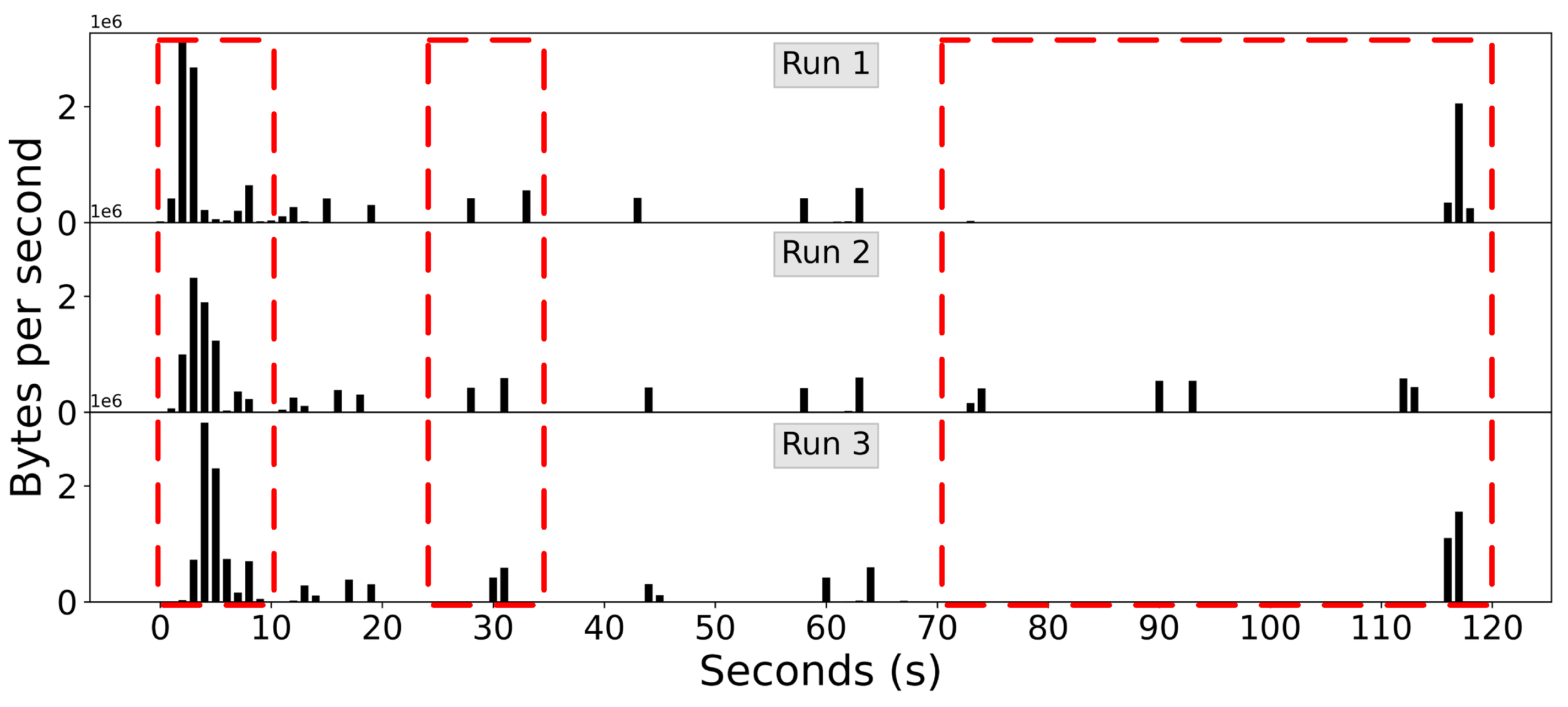
5.1. Bytes per Second (BPS)

Khan et al. [20,21] utilized this feature for video label prediction in encrypted network traffic for the first time. For the construction of the BPS, the network traffic was captured in the form of a packet capture file (PCAP), and the bytes received at every second were extracted as the the network traffic was captured. For a video spanning n seconds, the BPS sequence is defined as B = $(b_{t1},b_{t2},\dots ,b_{tn})$, where b is the number of bytes received at time t. The CNN model presented in [21] was used to train on the BPS dataset. The model achieved an accuracy of 73.07% over 100 epochs. The details of the CNN model are provided in

Table 1. Summary of the BPS classifier.

Layer ID	Layer (Type)	Output Shape	Param #
1	Conv1D	(None, 120, 1024)	7168
2	MaxPooling1D	(None, 60, 1024)	0
3	Conv1D	(None, 60, 512)	2097664
4	MaxPooling1D	(None, 30, 512)	0
5	Conv1D	(None, 30, 512)	1311232
6	MaxPooling1D	(None, 15, 512)	0
7	Dropout	(None, 15, 512)	0
8	Flatten	(None, 7680)	0
9	Dense	(None, Number of videos)	337964

Total parameters: 3,754,028; Trainable parameters: 3,754,028; Non-trainable parameters: 0.

.

5.2. Fingerprint of the Packet Size per Arrival Time (F-PAT)

In this technique, the packet sizes per arrival time was extracted from the dataset of PCAP files. For this purpose, Scapy was used to extract the packet information from the files. Similarly to the BPS, for any video v, the size of the packet per arrival time is indicated as P = $(pk{t}_{t1},pk{t}_{t2},\dots ,pk{t}_{tn})$, where pkt is the size of the packet at any time t. To eliminate abnormalities in the captured stream, a stable fingerprint can be created to overcome the problem [49]. For this purpose, the packet size of each segment was added separately. In this paper, the segment size of 6 s was selected, as discussed in [49]. The fingerprint of any consecutive segment of the PAT, that is, $s{g}_t$ and $s{g}_{t-1}$, can be created with the following formula.

$$f{p}_t=|s{g}_t-s{g}_{t-1}|$$

(3)

The created fingerprints were used to train the CNN model. Through rigorous experiments in which the hyper-parameter settings of the CNN were varied, the model achieved an accuracy of 75.88% with 300 epochs and with the ReLu activation function in all convolutional layers. The details of the CNN model used to train on the F-PAT dataset are provided in

Table 2. Summary of the F-PAT classifier.

Layer ID	Layer (Type)	Output Shape	Param #
1	Conv1D	(None, 21, 300)	1800
2	MaxPooling1D	(None, 21, 300)	0
3	Conv1D	(None, 21, 512)	461312
4	MaxPooling1D	(None, 10, 512)	0
5	Conv1D	(None, 10, 512)	262656
6	MaxPooling1D	(None, 10, 512)	0
7	Conv1D	(None, 10, 300)	153900
8	MaxPooling1D	(None, 10, 300)	0
9	Dropout	(None, 10, 300)	0
10	Flatten	(None, 3000)	0
11	Dense	(None, Number of videos)	129043

Total parameters: 1,008,711; Trainable parameters: 1,008,711; Non-trainable parameters: 0.

.

5.3. Fingerprint of the BPS (F-BPS)

To eliminate abnormalities in the BPS, a stable fingerprint of the BPS can be created by using the aforementioned technique. For this purpose, the BPS values of the segments were added, and a fingerprint of the segments of the BPS was created. Any two consecutive segments of the BPS $b{s}_t$ and $b{s}_{t-1}$ can be created with the following formula.

$$b{f}_t={\left(b{s}_t-b{s}_{t-1}\right)}^2$$

(4)

The only difference between the fingerprint of the PAT and BPS is that for F-BPS, the square of the difference between the two consecutive segments is taken. However, F-PAT is created by taking the absolute value of the difference. This is due to the elimination of the negative sign from the values. A CNN model with the same configuration used for the F-PAT was utilized to train on the F-BPS dataset. The only difference was that the Tanh activation function was used in the convolutional layers instead of ReLU. The model achieved an accuracy of 63.05%.

6. Results and Discussion

This section presents the results for the three aforementioned classifiers and the proposed E-Ensemble classifier. The classifiers were trained on the one-month dataset, and the 20-day datasets were tested for accuracy. After that, the classifier combination techniques discussed earlier were compared in order to obtain more accurate and stable results. Finally, the proposed classifier was compared with the individual classifiers competing in the construction of E-Ensemble.

6.1. Accuracy of Individual Classifiers on the 20-Day Dataset

This section presents the results of the individual classifiers trained on the month-wise dataset and tested on the day-wise dataset. From the results, it was observed that the standard deviation of the accuracy of the BPS classifier with respect to the F-PAT and F-BPS was 3.7. It is clear from the results that the BPS classifier showed more stable results than those of its counterparts. Moreover, the maximum variation in accuracy was observed on Day -20. Similarly, the standard deviations of the F-PAT and F-BPS were 6.61 and 4.17, respectively. The maximum differences between the F-PAT and F-BPS were 29.55% and 12.35%, respectively. The day-wise accuracy of the individual models is shown in

Table 3. Accuracy in % for the BPS, F-PAT, and F-BPS classifiers.

Dataset	BPS	F-PAT	F-BPS
Month	73.07	75.88	63.05
Day1	62.79	62.33	56.74
Day2	66.05	67.44	60.47
Day3	70.87	76.28	67.27
Day4	73.38	72.08	57.47
Day5	69.47	65.61	57.54
Day6	70.97	72.81	63.13
Day7	71.83	77.46	64.79
Day8	68.84	68.84	55.81
Day9	64.19	68.37	59.53
Day10	65.12	61.86	50.7
Day11	69.77	64.19	57.67
Day12	70	46.33	57.8
Day13	69.3	65.12	54.88
Day14	69.3	68.37	61.86
Day15	63.72	71.16	59.53
Day16	69.77	74.42	64.65
Day17	67.44	71.63	63.26
Day18	63.26	72.09	53.95
Day19	64.65	72.09	55.35
Day20	59.07	68.37	54.42

.

6.2. Comparison of Different Classifier Combination Techniques

This section presents the results of the proposed classifier, E-Ensemble, with different techniques for combining the classifiers. This experiment was performed to check which classifier combination technique showed more stable results. For this purpose, the aforementioned techniques, that is, the hard-level combination (majority voting) and soft-level combination (average voting), were utilized. The same method was used for evaluation purposes. The classifier was trained on the month-wise dataset and tested on the day-wise dataset. From the results, it was observed that the average voting technique outperformed the majority voting technique in all day-wise datasets, as shown in Figure 9. Furthermore, the results also showed that the average voting technique was more stable, since it had the lowest standard deviation of 2.96, unlike the majority voting, which had a standard deviation of 4.17. Furthermore, average voting showed a high accuracy of 81.81% in comparison with majority voting, which had an accuracy of 75.58%.

6.3. Comparison of the Individual Classifiers with the Average Voting Technique

In this section, we present a comparison of the accuracy of the individual classifiers with the averaging voting technique. From the results, it was observed that the average voting technique outperformed all classifiers. Moreover, it was also observed that even if the component classifiers’ accuracy was lower, the average voting technique identified the videos with a high accuracy, as shown in Figure 10 on Day-10 and Day-12.

We conclude this section on the results with the following observations. The soft-level classifier combination technique performed better than the hard-level classifier combination technique for video identification in network traffic. Individually, the BPS classifier showed better performance than that of the F-PAT and F-BPS classifiers. However, the E-Ensemble classifier that was a soft-level combination of the BPS, F-PAT, and F-BPS classifiers performed even better than the individual classifiers.

7. Conclusions

An ensemble classifier has superior classification performance to that of an individual classifier. Taking advantage of an ensemble classifier, this paper presents a novel E-Ensemble classifier that predicts videos in encrypted network traffic. For this purpose, two classifier combination techniques were used to determine which technique provided the most stable results. The datasets used in this paper were created at two different dates and times. For the first dataset, the video streams were captured over a whole month. For the second dataset, the video streams were captured over 20 days. E-Ensemble was trained on the dataset of the month, and its accuracy was tested on the other dataset. The results showed that E-Ensemble outperformed the individual classifiers, even if the accuracy of its component classifiers was lower. Moreover, the results also showed that the soft-level classifier combination technique displayed more accurate and stable results, with a high accuracy of 81.81%.

References

1. Ledwich, M.; Zaitsev, A. Algorithmic extremism: Examining YouTube’s rabbit hole of radicalization. arXiv 2019, arXiv:1912.11211. [Google Scholar] [CrossRef] [Green Version]
2. Buntain, C.; Bonneau, R.; Nagler, J.; Tucker, J.A. YouTube recommendations and effects on sharing across online social platforms. Proc. Acm-Hum.-Comput. Interact. 2021, 5, 1–26. [Google Scholar] [CrossRef]
3. Heuer, H.; Hoch, H.; Breiter, A.; Theocharis, Y. Auditing the biases enacted by YouTube for political topics in Germany. In Proceedings of the Mensch und Computer 2021, Ingolstadt, Germany, 5–8 September 2021; pp. 456–468. [Google Scholar]
4. Bromell, D. After Christchurch: Hate, Harm and the Limits of Censorship; Victoria University of Wellington: Wellington, New Zealand, 2021. [Google Scholar]
5. Solsman, J.E. YouTube’s AI Is the Puppet Master over Most of What You Watch. 2018. Available online: https://www.cnet.com/news/youtube-ces-2018-neal-mohan (accessed on 1 November 2022).
6. Creators, Y. How YouTube’s Home Screen Works. 2017. Available online: https://www.youtube.com/watch?v=69tpVNunQEU (accessed on 1 November 2022).
7. Bremler-Barr, A.; Harchol, Y.; Hay, D.; Koral, Y. Deep packet inspection as a service. In Proceedings of the 10th ACM International on Conference on Emerging Networking Experiments and Technologies, Sydney, Australia, 2–5 December 2014; pp. 271–282. [Google Scholar]
8. Khan, M.U.S.; Abbas, A.; Ali, M.; Jawad, M.; Khan, S.U. Convolutional Neural Networks as Means to Identify Apposite Sensor Combination for Human Activity Recognition. In Proceedings of the 2018 IEEE/ACM International Conference on Connected Health: Applications, Systems and Engineering Technologies (CHASE), Washington, DC, USA, 26–28 September 2018; pp. 45–50. [Google Scholar]
9. Hassan, S.U.; Saleem, A.; Soroya, S.H.; Safder, I.; Iqbal, S.; Jamil, S.; Bukhari, F.; Aljohani, N.R.; Nawaz, R. Sentiment analysis of tweets through Altmetrics: A machine learning approach. J. Inf. Sci. 2021, 47, 712–726. [Google Scholar] [CrossRef]
10. Hassan, S.U.; Shabbir, M.; Iqbal, S.; Said, A.; Kamiran, F.; Nawaz, R.; Saif, U. Leveraging deep learning and SNA approaches for smart city policing in the developing world. Int. J. Inf. Manag. 2021, 56, 102045. [Google Scholar] [CrossRef]
11. Said, A.; Hassan, S.U.; Tuarob, S.; Nawaz, R.; Shabbir, M. DGSD: Distributed graph representation via graph statistical properties. Future Gener. Comput. Syst. 2021, 119, 166–175. [Google Scholar] [CrossRef]
12. Waheed, H.; Anas, M.; Hassan, S.U.; Aljohani, N.R.; Alelyani, S.; Edifor, E.E.; Nawaz, R. Balancing sequential data to predict students at-risk using adversarial networks. Comput. Electr. Eng. 2021, 93, 107274. [Google Scholar] [CrossRef]
13. Waheed, H.; Hassan, S.U.; Aljohani, N.R.; Hardman, J.; Alelyani, S.; Nawaz, R. Predicting academic performance of students from VLE big data using deep learning models. Comput. Hum. Behav. 2020, 104, 106189. [Google Scholar] [CrossRef] [Green Version]
14. Wang, X.; Rak, R.; Restificar, A.; Nobata, C.; Rupp, C.; Batista-Navarro, R.T.B.; Nawaz, R.; Ananiadou, S. Detecting experimental techniques and selecting relevant documents for protein-protein interactions from biomedical literature. BMC Bioinform. 2011, 12, 1–13. [Google Scholar] [CrossRef] [Green Version]
15. Nawaz, R.; Thompson, P.; Ananiadou, S. Negated bio-events: Analysis and identification. BMC Bioinform. 2013, 14, 1–21. [Google Scholar] [CrossRef] [Green Version]
16. Khan, M.U.S.; Abbas, A.; Rehman, A.; Nawaz, R. HateClassify: A Service Framework for Hate Speech Identification on Social Media. IEEE Internet Comput. 2021, 25, 40–49. [Google Scholar] [CrossRef]
17. Nawaz, R.; Sun, Q.; Shardlow, M.; Kontonatsios, G.; Aljohani, N.R.; Visvizi, A.; Hassan, S.U. Leveraging AI and Machine Learning for National Student Survey: Actionable Insights from Textual Feedback to Enhance Quality of Teaching and Learning in UK’s Higher Education. Appl. Sci. 2022, 12, 514. [Google Scholar] [CrossRef]
18. Thompson, P.; Nawaz, R.; Korkontzelos, I.; Black, W.; McNaught, J.; Ananiadou, S. News search using discourse analytics. In Proceedings of the 2013 Digital Heritage International Congress (Digital Heritage), Marseille, France, 28 October–1 November 2013; Volume 1, pp. 597–604. [Google Scholar]
19. Nawaz, R.; Thompson, P.; McNaught, J.; Ananiadou, S. Meta-knowledge annotation of bio-events. In Proceedings of the Proceedings of the Seventh International Conference on Language Resources and Evaluation (LREC’10), Valletta, Malta, 17–23 May 2010. [Google Scholar]
20. Khan, M.U.; Bukhari, S.M.; Maqsood, T.; Fayyaz, M.A.; Dancey, D.; Nawaz, R. SCNN-Attack: A Side-Channel Attack to Identify YouTube Videos in a VPN and Non-VPN Network Traffic. Electronics 2022, 11, 350. [Google Scholar] [CrossRef]
21. Khan, M.U.; Bukhari, S.M.; Khan, S.A.; Maqsood, T. ISP can identify YouTube videos that you just watched. In Proceedings of the 2021 International Conference on Frontiers of Information Technology (FIT), Islamabad, Pakistan, 13–14 December 2021; pp. 1–6. [Google Scholar]
22. Schuster, R.; Shmatikov, V.; Tromer, E. Beauty and the burst: Remote identification of encrypted video streams. In Proceedings of the 26th USENIX Security Symposium (USENIX Security 17), Vancouver, BC, Canada, 16–18 August 2017; pp. 1357–1374. [Google Scholar]
23. Dietterich, T.G. Ensemble methods in machine learning. In Proceedings of the International Workshop on Multiple Classifier Systems, Cagliari, Italy, 21–23 June 2000; pp. 1–15. [Google Scholar]
24. Chaudhary, A.; Kolhe, S.; Kamal, R. A hybrid ensemble for classification in multiclass datasets: An application to oilseed disease dataset. Comput. Electron. Agric. 2016, 124, 65–72. [Google Scholar] [CrossRef]
25. Cai, Y.; Liu, X.; Zhang, Y.; Cai, Z. Hierarchical ensemble of extreme learning machine. Pattern Recognit. Lett. 2018, 116, 101–106. [Google Scholar] [CrossRef]
26. Drotár, P.; Gazda, M.; Vokorokos, L. Ensemble feature selection using election methods and ranker clustering. Inf. Sci. 2019, 480, 365–380. [Google Scholar] [CrossRef]
27. Wang, Y.; Wang, D.; Geng, N.; Wang, Y.; Yin, Y.; Jin, Y. Stacking-based ensemble learning of decision trees for interpretable prostate cancer detection. Appl. Soft Comput. 2019, 77, 188–204. [Google Scholar] [CrossRef]
28. Abuassba, A.O.; Zhang, D.; Luo, X.; Shaheryar, A.; Ali, H. Improving classification performance through an advanced ensemble based heterogeneous extreme learning machines. Comput. Intell. Neurosci. 2017, 2017. [Google Scholar] [CrossRef] [PubMed] [Green Version]
29. Moustafa, S.; ElNainay, M.Y.; El Makky, N.; Abougabal, M.S. Software bug prediction using weighted majority voting techniques. Alex. Eng. J. 2018, 57, 2763–2774. [Google Scholar] [CrossRef]
30. Valstar, M.F.; Jiang, B.; Mehu, M.; Pantic, M.; Scherer, K. The first facial expression recognition and analysis challenge. In Proceedings of the 2011 IEEE International Conference on Automatic Face & Gesture Recognition (FG), Santa Barbara, CA, USA, 21–25 March 2011; pp. 921–926. [Google Scholar]
31. Duro, D.C.; Franklin, S.E.; Dubé, M.G. A comparison of pixel-based and object-based image analysis with selected machine learning algorithms for the classification of agricultural landscapes using SPOT-5 HRG imagery. Remote Sens. Environ. 2012, 118, 259–272. [Google Scholar] [CrossRef]
32. Prasad, B.; Prasad, P.; Sagar, Y. A comparative study of machine learning algorithms as expert systems in medical diagnosis (Asthma). In Proceedings of the International Conference on Computer Science and Information Technology, Chengdu, China, 10–12 June 2011; pp. 570–576. [Google Scholar]
33. Zhenxiang, L.; Mingbo, H.; Song, L.; Xin, W. Research of P2P traffic comprehensive identification method. In Proceedings of the 2011 International Conference on Network Computing and Information Security, Guilin, China, 14–15 May 2011; Volume 1, pp. 307–310. [Google Scholar]
34. Afandi, W.; Bukhari, S.M.; Khan, M.U.; Maqsood, T.; Khan, S.U. A Bucket-Based Data Pre-Processing Method for Encrypted Video Detection. In Proceedings of the 35th International Conference on Computer Applications in Industry and Engineering (CAINE), Online, 17–19 October 2022. [Google Scholar]
35. Akdemir, B.; Kara, S.; Polat, K.; Güven, A.; Güneş, S. Ensemble adaptive network-based fuzzy inference system with weighted arithmetical mean and application to diagnosis of optic nerve disease from visual-evoked potential signals. Artif. Intell. Med. 2008, 43, 141–149. [Google Scholar] [CrossRef]
36. Song, X.; Jiao, L.; Yang, S.; Zhang, X.; Shang, F. Sparse coding and classifier ensemble based multi-instance learning for image categorization. Signal Process. 2013, 93, 1–11. [Google Scholar] [CrossRef]
37. Glodek, M.; Reuter, S.; Schels, M.; Dietmayer, K.; Schwenker, F. Kalman filter based classifier fusion for affective state recognition. In Proceedings of the International Workshop on Multiple Classifier Systems, Nanjing, China, 15–17 May 2013; pp. 85–94. [Google Scholar]
38. Klement, W.; Wilk, S.; Michalowski, W.; Farion, K.J.; Osmond, M.H.; Verter, V. Predicting the need for CT imaging in children with minor head injury using an ensemble of Naive Bayes classifiers. Artif. Intell. Med. 2012, 54, 163–170. [Google Scholar] [CrossRef] [PubMed]
39. Gómez, S.E.; Martínez, B.C.; Sánchez-Esguevillas, A.J.; Callejo, L.H. Ensemble network traffic classification: Algorithm comparison and novel ensemble scheme proposal. Comput. Netw. 2017, 127, 68–80. [Google Scholar] [CrossRef]
40. He, H.; Luo, X.; Ma, F.; Che, C.; Wang, J. Network traffic classification based on ensemble learning and co-training. Sci. China Ser. F Inf. Sci. 2009, 52, 338–346. [Google Scholar] [CrossRef]
41. Wang, C.; Guan, X.; Qin, T. A traffic classification approach based on characteristics of subflows and ensemble learning. In Proceedings of the 2017 IFIP/IEEE Symposium on Integrated Network and Service Management (IM), Lisbon, Portugal, 8–12 May 2017; pp. 588–591. [Google Scholar]
42. Dvir, A.; Marnerides, A.K.; Dubin, R.; Golan, N. Clustering the unknown-the youtube case. In Proceedings of the 2019 International Conference on Computing, Networking and Communications (ICNC), Honolulu, HI, USA, 18–21 February 2019; pp. 402–407. [Google Scholar]
43. Fayyaz, M.A.B.; Johnson, C. Object detection at level crossing using deep learning. Micromachines 2020, 11, 1055. [Google Scholar] [CrossRef]
44. Kamal, A.S.; Bukhari, S.M.A.H.; Khan, M.U.S.; Maqsood, T.; Fayyaz, M. Traffic Pattern Plot: Video Identification in Encrypted Network Traffic. 2022. Available online: https://www.researchgate.net/publication/362761222_Traffic_Pattern_Plot_Video_Identification_in_Encrypted_Network_Traffic (accessed on 1 November 2022).
45. Mohandes, M.; Deriche, M.; Aliyu, S.O. Classifiers combination techniques: A comprehensive review. IEEE Access 2018, 6, 19626–19639. [Google Scholar] [CrossRef]
46. Kuncheva, L.I. Combining Pattern Classifiers: Methods and Algorithms; John Wiley & Sons: Hoboken, NJ, USA, 2014. [Google Scholar]
47. Kittler, J.; Hatef, M.; Duin, R.P.; Matas, J. On combining classifiers. IEEE Trans. Pattern Anal. Mach. Intell. 1998, 20, 226–239. [Google Scholar] [CrossRef] [Green Version]
48. Delgado, R. A semi-hard voting combiner scheme to ensemble multi-class probabilistic classifiers. Appl. Intell. 2022, 52, 3653–3677. [Google Scholar] [CrossRef]
49. Gu, J.; Wang, J.; Yu, Z.; Shen, K. Walls have ears: Traffic-based side-channel attack in video streaming. In Proceedings of the IEEE INFOCOM 2018-IEEE Conference on Computer Communications, Honolulu, HI, USA, 16–19 April 2018; pp. 1538–1546. [Google Scholar]
Figure 1. Abnormalities in streaming patterns.
Electronics 11 04076 g001
Figure 2. Abnormalities in accuracy due to VBR encoding.
Electronics 11 04076 g002
Figure 3. General architecture of an ensemble classifier.
Electronics 11 04076 g003
Figure 4. An ensemble classifier based on a hard-level combination.
Electronics 11 04076 g004
Figure 5. Example of hard-level voting.
Electronics 11 04076 g005
Figure 6. Ensemble classifier based on a soft-level combination.
Electronics 11 04076 g006
Figure 7. Example of a soft-level combination in which the average rule is applied.
Electronics 11 04076 g007
Figure 8. A detailed overview of the E-Ensemble classifier.
Electronics 11 04076 g008
Figure 9. Accuracy in % of for majority voting and average voting.
Electronics 11 04076 g009
Figure 10. Accuracy in % of the individual classifiers and the average voting technique.
Electronics 11 04076 g010