Article

Deep Learning-Based Modulation Recognition for Low Signal-to-Noise Ratio Environments

1
The 40th&41th Research Institute, China Electronics Technology Group Corporation, Beijing 100846, China
2
School of Telecommunications Engineering, Xidian University, Xi’an 710071, China
*
Author to whom correspondence should be addressed.
These authors contributed equally to this work.
Electronics 2022, 11(23), 4026; https://doi.org/10.3390/electronics11234026
Submission received: 1 November 2022 / Revised: 21 November 2022 / Accepted: 23 November 2022 / Published: 5 December 2022
(This article belongs to the Special Issue Advances and Applications of Networking and Multimedia Technologies)

Abstract

:
Automatic modulation classification (AMC), which plays a significant role in wireless communication, can recognize the modulation type of the received signal without large amounts of transmitted data and parameter information. Supported by deep learning, which is a powerful tool for functional expression and feature extraction, the development of AMC can be greatly promoted. In this paper, we propose a deep learning-based modulation classification method with 2D time-frequency signal representation. In our proposed method, signals which have been received are first analyzed by time-frequency based on continuous wavelet transform (CWT). Then, CWT images of received signals are obtained and input to the deep learning model for classifying. We create a new CWT image dataset including 12 modulation types of signals under various signal-to-noise ratio (SNR) environment to verify the effectiveness of the proposed method. The experimental results demonstrate that our proposed method can reach to a high classification accuracy over the SNR of −11 dB.

1. Introduction

The modulation signal is a significant research object in wireless communication and radar systems. To obtain the required signal, signal modulation classification is a key technology, which is intended to identify the modulation information of the received signal. It is also an essential process in cognitive radio systems to identify the modulation type from the received signal, which is because the modulation scheme must be first identified before the receiver can extract information from the received signal. Modulation classification has a wide range of applications, such as signal demodulation [1,2,3,4], anomaly detection [5,6,7,8], and interference location [9,10,11].
Previous works on modulation classification can be mainly categorized into two classes: methods based on likelihood function and methods based on signal features [12].
For likelihood-based methods, it can be regarded as a problem of multiple hypothesis testing. In this kind of method, the probability density function of the received signal is considered that has abundant information for classification. Panagiotou et al. [13] proposed two algorithms for modulation classification, which are the generalized likelihood ratio test-based method and hybrid likelihood ratio test-based method. Abdi et al. [14], respectively, proposed an average likelihood ratio-based and a quasi-hybrid likelihood ratio-based signal modulation classification method for noisy channels and Rayleigh fading channels. Dobre and Hameed [15] compared the performance of a hybrid likelihood ratio test-based classifier and a quasi-hybrid likelihood ratio test-based classifier, and concluded that the two methods perform similarly, but the computation complexity of the latter was lower. However, methods based on likelihood function usually require prior information, which is actually difficult to obtain in modulation classification and the derivation of likelihood function is complicated and computationally intensive.
Feature-based modulation classification methods are commonly used in practice due to low-complexity calculations and no prior knowledge being necessary [16]. Zhang et al. [17] derived the higher-order cumulants as classifying features from received signals and constructed a support vector machine-based classification model. Yan et al. [18] proposed a graph-based method for signal modulation classification, which constructed the most discriminative features by Kullback–Leibler divergence and used the Hamming distance between features for classification. However, it is sometimes difficult with these methods to extract features facing low SNR environment. When high ambiguity signals are used to process, a large number of unpredictable results will be produced.
With the rapid development of deep learning, which is a powerful tool for functional expression and feature extraction, it has been widely applied in the field of wireless communication [19,20,21,22]. Based on deep learning, many issues of traditional modulation classification can be solved, such as high dependence on artificial features, low model robustness and high model complexity. Thus, many studies have adopted deep learning methods, especially CNN-based methods [23,24]. Meanwhile, the application of deep CNNs with various 2D time-frequency signal representations has become a hot research topic recently. In [25], three time-frequency representations of the audio signal, respectively, calculated by CWT, Mel-spectrograms, and Gammatone spectrograms are combined together to conduct speech analysis. Furthermore, a CNN model was proposed to learn different representations of the audio signal. Khare et al. [26] proposed a smoothed pseudo-Wigner-Ville distribution to transfer time-domain filtered EEG signals into a time–frequency representation and use configurable CNN to conduct emotion identification. A deep CNN classification algorithm with time-frequency representations of Cohen’s class was proposed in [27], which greatly improves the model performance.
In this paper, we propose a novel modulation classification method based on deep learning, which considers time-frequency characteristics of signals as classifying features. In the electromagnetic environment of low SNR, the classification accuracy of the intercepted original signal is low, and it takes a lot of time to extract its features. Therefore, how to analyze and transform the original signal and obtain its effective features for recognition and classification is a key problem to be solved. Aiming at this, we use a time-frequency analysis method of electromagnetic signals based on continuous wavelet transform (CWT). That is, CWT images of modulation signals can be obtained through the time-frequency conversion to obtain their characteristic information. Specifically, CWT-based time-frequency analysis is carried out previously on the received signal to obtain its CWT image. Related experiments appear that CWT images of different modulation types of signals after time-frequency analysis are distinguishable, and the transformed images still retain relatively complete feature information. Therefore, we use these CWT images as the input of the deep learning model for classification to obtain the type and modulation information of the received signal.
The contributions of this paper can be summarized as follows:
  • We propose a novel modulation classification method based on deep learning, which considers time-frequency characteristics of signals as classifying features.
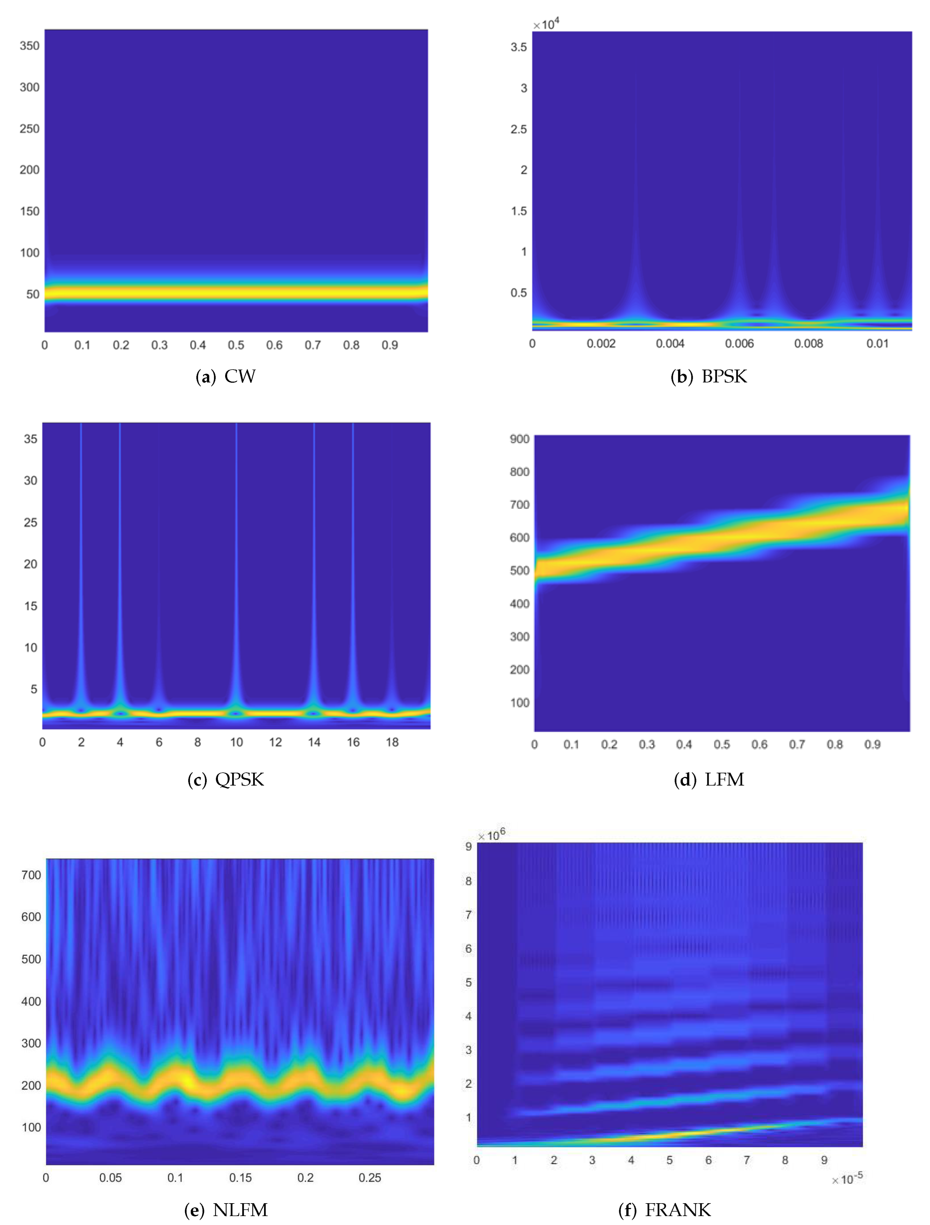
  • We carry out time-frequency analysis of the signal and transform the original received signals into CWT images which are distinguishable and feature informative.
  • We conduct experiments to test the performance of our proposed method and the experimental results show that the model reaches to 95% accuracy which demonstrates the effectiveness of our proposed method.
The main structure of this paper is organized as follows. In Section 2, some related studies are briefly introduced, especially CNN-based signal modulation classification. In Section 3, we present the proposed method in detail by giving the specific formulaic description of CWT and the structure of designed CNN network. Meanwhile, the process of CWT dataset generation is also presented in this section. In Section 4, we represent some experimental results demonstrating that the classification accuracy of our proposed method can reach to 90% over the SNR of −11 dB. Meanwhile, we give some analysis on the reason why there is an accuracy drop when the SNR is extremely low.

2. Related Work

Deep learning-based modulation classification methods have been widely investigated in recent years. Convolutional neural network (CNN) demonstrated satisfactory performance in a wide variety of research tasks, and many CNN-based modulation classification methods have been proposed. O’Shea et al. [28] first applied CNN to the task of radio modulation classification and, respectively, investigated the performance of the common feature-based method and the expert feature-based method. For easier deployment of the deep learning model on devices which have some resource constrains, Zhang et al. [29] proposed the Average Percentage of Zeros (APoZ) algorithm to slim the structure of traditional CNN which cannot just reduce the network size and computational cost, but can also improve the stability of the average error of the network. Similarly, Ji et al. [30] proposed a hybrid pruning method which can be achieved by the simultaneous enforcement of layer and channel level sparsity. Xu et al. [31] proposed an automatic modulation recognition (AMR) method based on temporal convolutional network (TC-AMRNet) with real-time for 5G low-latency services. Motivated by facial recognition, Zhang et al. [32] proposed a multi-scale network for AMC task to solve the problem of intra-class diversity in wireless communication environment.
To explore more distinguishing information for modulation classification and to improve the accuracy of the classification model, some studies adopted an attention mechanism for feature extraction. Wei et al. [33] proposed a novel modulation classification framework with self-attention mechanism, which consisted of a shallow CNN, a bidirectional long short-term memory (Bi-LSTM) network, and a dense neural network (DNN). Liang et al. [34] proposed a deep learning-based end-to-end framework for AMR, which combined complex-valued CNN with the feature calibration module to emphasize the more relevant features. Gupta et al. [35] similarly introduced an attention mechanism into the deep modulation classification model to focus on certain distinguishing regions which can effectively help improve the classification efficiency and accuracy. To deal with the problem of channel deterioration, Huynh-The et al. [36] proposed a novel CNN architecture with high performance, which consists of multiple feature learning blocks. In their method, every block contains an attention and skip connection to constantly focus on relevant features.
Due to the complication of the wireless communication environment, it is difficult to directly perform modulation classification on the received signals. Therefore, some studies adopted different pre-processing method before actual classifying. Hao et al. [37] previously conducted signal frequency domain analysis based on Fast Fourier Transformation (FFT) and obtained a great accuracy gain compared with other traditional algorithms without pre-processing. Similarly, Yakkati et al. [38] considered previous signal analysis based on the fixed boundary range-based empirical wavelet transform to obtain the sub-band signals for classifying. Liang et al. [39] used short-time Fourier transform (STFT) to obtain time-frequency images of the received signals, which will be input into the ResNeXt network for modulation classification. Li and Shi [40] transformed the one-dimensional signals into specific images by pseudo Wigner-Ville distribution and adopted feature fusion scheme to tackle the modulation classification task, which aims to fuse features extracted by multiple different CNN.
Moreover, many deep learning-based AMC frameworks were studied in recent years. A modular few-shot learning framework for signal modulation classification is proposed in [41], which includes and IQ fusion module, a graph convolution neural network (GCNN)-based module and a classifying module, and related experiments demonstrated excellent performance of the proposed method. Huang et al. [42] proposed a cascaded CNN-based AMC scheme, namely CasCNN. There are two CNN blocks in CasCNN which are, respectively, responsible for inter-class classification and intra-class classification. Considering the difficulty of manually designing the deep neural network, Zhang et al. [43] proposed a neural architecture search method for modulation recognition, which can automatically fix the model structure and parameters. Considering the problem of data leakage brought by conventional deep learning-based method, Wang et al. [44] proposed a novel modulation classification method based on federated learning framework and introduced balanced cross entropy loss to deal with the problem of data heterogeneity of local clients.

3. Materials and Methods

3.1. Time-Frequency Representation

CWT, which is a time-frequency analysis approach, has the ability to characterize the local characteristics of the signal in both time and frequency domains. It is suitable for detecting the instantaneous abnormal phenomenon of entrainment in normal signal and displaying its composition.
Previously, we generated 12 kinds of modulation signals in a range of SNRs from −15 dB to 10 dB with a 1 dB step, including NLFM, LFM, BPSK, QPSK, Frank, FSK, CW, Costas, P1, P2, P3, and P4. For each signal, it can be represented as
f ( t ) = x ( t ) + σ ω ( t ) ,
where ω ( t ) , σ and x ( t ) , respectively, denotes white Gaussian noise, noise level and electromagnetic signal. Then, CWT-based time-frequency analysis is performed to transfer each original signal into CWT image. The formulaic detailed description of CWT is as follows:
First we introduce the window function ψ a , b
ψ a , b t = 1 / | a | ψ t b / a ,
where ψ ( t ) is the selected mother wavelet, and ψ a , b ( t ) is the mother sequence obtained after scaling and shifting of the basic wavelet, which plays the role of observation window for the analyzed signal. The degree of scaling and translation is determined by a and b. a is the scale factor, representing the scaling related to frequency. a R and a 0 . b is the time shifting factor. At the same time, to ensure that the time window and frequency window have fast attenuation characteristics, the basic wavelet ψ ( t ) is often required to have the following properties:
ψ t | C 1 + | t | 1 ε , | ψ ^ ω ¯ | C 1 + | ω | 1 ε ,
where ψ ^ ω ¯ is the Fourier transform of ψ ( t ) . ϵ > 0 , and C is a constant which is independent of x and ω ¯ .
The essence of CWT is to decompose the original time-domain signal into a series of wavelet transform coefficients W ψ f a , b by performing the inner product operation on the specific wavelet ϕ ( t ) , thereby constructing a time-frequency signal with good localization in time domain and frequency domain. For achieving the CWT of a modulation signal f ( x ) , a mother analyzing wavelet has to be chosen initially. Therefore, we can merely consider the choice of the mother wavelet to conduct CWT. In our method, we adopt Morlet [45] as the mother wavelet since it is the typical function used by many wavelet transform-based studies [46,47,48]. The mathematical representation of Morlet is
ψ t = π 1 / 4 e r 2 / 2 cos ω 0 t
where ω 0 denotes the central frequency of ϕ ( t ) . Then, the CWT function can be defined as
W ψ f a , b = 1 | a | + + f t ψ t b a d t
The principal role of CWT is to pay more attention to the shape of the signal in time and frequency domains, which is conducive to the subsequent work of the classifier. As can be observed from Figure 1, the CWT image can retain relatively complete feature information of the signal. As can be observed in Figure 2, the upper parts of CWT images are mainly noise, and the lower parts are the original signals. Furthermore, by comparing the signal parts of these CWT images, it can be found that even though under noisy environment, CWT images of these signals have certain differences, which are mainly caused by the characteristics of these modulation signals in time-frequency domain. Therefore, the CWT image of the signal can be used as the input of the deep learning network to extract relevant features for modulation classification.

3.2. System Model

3.2.1. Overview

CNN is widely used for image processing, especially in image classification. Based on LeNet [49], we propose an effective framework to classify the CWT images. As shown in Figure 3, our proposed framework consists of three stages. The input image comes from CWT dataset, which is resized to 32 × 32 .

3.2.2. PreConv

The first stage contains a PreConv Block, a 5 × 5 convolution layer and a maximum pooling layer. The input image first passes through the PreConv Block. As shown in Figure 4, the PreConv Block is composed of a 3 × 1 regular convolution, a 1 × 3 regular convolution and a 1 × 1 regular convolution. Assuming that the X denotes the input image, F 1 × 1 denotes the output feature map of 1 × 1 convolution, F 1 × 3 denotes the output feature map of 1 × 3 convolution and F 3 × 1 denotes the output feature map of 3 × 1 convolution. The final output feature map F o of PreConv Block can be expressed as
F o = F 1 × 1 F 1 × 3 F 3 × 1 ,
where ⊕ means element-wise addition. By merging the output feature maps of the three convolution kernels, the low-level features of the input image can be enhanced. Then we use a 5 × 5 with stride 2 to reduce the feature dimension. After the maximum pooling layer, we can obtain the output feature map of the stage 1, whose resolution is 14 × 14 .

3.2.3. Diverse Block

In the second stage, inspired by the Inception Module [50], we design the Diverse Block to enrich the feature space by using multi-branch structures. The Diverse Block contains four branches, as Figure 5. The first branch with a 1 × 1 convolution can be treated as the skip connection, which is similar to Resnet [51]. The second branch with a 1 × 1 convolution and a 3 × 3 convolution can be treated as an enhanced 3 × 3 convolution. Assuming that the input feature map is X, F 1 × 1 is 1 × 1 convolution and F 3 × 3 is 3 × 3 convolution. The output feature map of this branch is
F o = X F 1 × 1 F 3 × 3 ,
where ⊛ means the convolution operator. As X F 1 × 1 is 1 × 1 convolution, which performs only channel-wise linear combination but no spatial aggregation. We can recombine the 1 × 1 convolution to merge it into 3 × 3 convolution. The merge convolution F m e r g e can be given by:
F m e r g e = T R A N S ( F 1 × 1 ) F 3 × 3 ,
where T R A N S ( F 1 × 1 ) is the tensor transposed from F 1 × 1 .
Similarly, the third branch with a 1 × 1 convolution and average pooling can be treated as a 3 × 3 convolution. The average pooling can be transformed as a 3 × 3 convolution, whose kernel F R C × C × 3 × 3 is
F d , c , 3 , 3 = 1 3 2 if d = c , 0 elsewise .
These four branches can be concatenated to enrich the feature space of the output feature map, which contains both local features and non-local features. After stage 2, the resolution of the feature map is 5 × 5 .

3.2.4. Loss

The last stage contains three parts: flatten, dense and softmax. The final merged feature map will be flattened to a 1 D feature with the resolution of 1 × 1 × 400 . Then the flattened feature will pass through a dense layer to reduce dimensions. Finally, we use the softmax layer to normalize the features, which can map the probability corresponding to each modulation type. After the softmax layer, the final normalized likelihood vector P = [ P 1 , P 2 , , P m ] can be computed by
P = s o f t m a x ( X ) ,
where X is the input feature map of the softmax layer. The modulation type of received signals can then be determined based on the maximum probability, given as
y ^ = a r g m a x m = 1 , 2 , , M ( P m ) ,
where y ^ is the predicted label.
We use the cross-entropy function as our loss function, which can be formulated as
L o s s = 1 M i = 1 M y i × l n y ^ i ,
where y i is the target label, y ^ i is the predicted label and M is the sum of modulation types.

4. Results and Discussion

4.1. Implementation Details

We generated a new CWT dataset to verify the effectiveness of our method. Specifically, our CWT dataset consists of 12 modulations (NLFM, LFM, BPSK, QPSK, Frank, FSK, CW, Costas, P1, P2, P3, and P4) under an SNR range from −15 dB to 10 dB with a 1 dB step. For the training set, there are 520 CWT image samples for each type of modulation signal under different SNRs. Furthermore, each modulation type has 20 samples under each SNR level. For test set, there are 260 CWT image samples for each type of modulation signals under different SNRs. Thus, the whole dataset consists of a training set with a total number of 6240 images and a test set with a total number of 3120 images. The size of each CWT image was uniformly adjusted to 32 × 32, and a total of 1000 training epochs were set. In addition, we used the Adam optimizer as the training method.

4.2. Experimental Section

The accuracy and loss values of each round of training and testing are shown in Figure 6. With the increase of training times, the accuracy gradually increases while the loss value gradually decreases. When it is around the 500th epoch, the loss value begins to converge, and when the 300th epoch is reached, the accuracy basically stabilizes and reaches to approximately 100%. By using the K-fold cross-validation method, we randomly divide the training data into k without repetition, among which k 1 is used for model training and the remaining one is used for model testing. This process is repeated for k times to obtain k models and their performance evaluation. Specifically, we set k as 10 and conducted 10 times training. As Figure 7 shows, the model has an average cross-validation accuracy over 80%. The key point of this method is that after the data set is divided into k pieces, different blocks are selected each time as the verification set in the cross-validation to ensure that there will be no duplicate verification set, which can better evaluate the performance of model.
As Figure 8 shows, we segmented the dataset according to each SNR level to verify the effectiveness of the deep learning modulation classification method proposed in this paper. As we can see in the figure, the model has a higher recognition accuracy when the value of SNR is higher, and it has the accuracy over 90% while the value of SNR is over −11 dB. However, the accuracy is relatively low under SNRs from −15 dB to −12 dB and the model only has the accuracy about 75% under the lowest SNR of −15 dB. On the whole, the model has an excellent performance and high classification accuracy under the SNR over −11 dB but has an accuracy drop when the SNR is under −11 dB. To further evaluate the effectiveness of our method, we did some extensive experiments.
The recognition accuracies for each type of modulation signal with the SNR of −15 dB to 10 dB are demonstrated in Figure 9, Figure 10 and Figure 11. It can be seen from the figures that when the SNR is lower than 0 dB, the accuracy of some particular modulation signals, such as P1, P2, P3, and P4, is low. This is because when the SNR is low, the signal has serious distortion and the noise characteristics are more significant, which has a greater impact on the recognition results. Moreover, the choice of a mother wavelet for CWT is also an important factor which can influence the recognition accuracy.
The signal detection rate means that when there is a signal at the receiver input, due to interference background and other reasons, two kinds of decisions may be made: 1. There is a signal; 2. No signal (or noise signal). It depends on the characteristics of the signal and noise, the characteristics of the receiver and the set threshold. The error rate refers to the probability that when a threshold detection method is used in radar detection, due to the widespread existence and fluctuation of noise, there is no target, but it is judged to be a target. We use these two indicators to evaluate the detection efficiency of our proposed method. The results are shown in Figure 12.
In the process of signal recognition, we use the classification confidence of the model as the threshold to detect the false alarm probability. It can be seen from Figure 12 that the higher the threshold, the lower the false alarm probability. After the threshold exceeds 0.999, the false alarm probability is 0. Signal detection probability refers to the probability of detecting a signal as a “signal” rather than a “noise”. Its value is related to the set threshold. The larger the threshold, the smaller the detection probability. When the threshold is set to 0.8, the detection probability can reach 96%.

5. Conclusions

In this paper, we proposed a novel deep learning-based signal modulation classification method, which considers time-frequency characteristics of signals as classifying features. First, CWT-based time-frequency analysis is performed on the received signal to obtain its CWT image. Then, the CWT image is input into the proposed deep learning model for classifying to obtain the type and modulation information of the received signal. To verify our proposed method, we created a new CWT image dataset including 12 types of modulation signals under a range of SNRs from −15 dB to 10 dB, and conducted experiments to test our classifying model on this dataset. The experimental results show that the model the accuracy over 90% while the value of SNR is over −11 dB and has the accuracy over 75% under the lower range of SNRs from −15 dB to −12 dB. However, there remain some limitations, such as inevitable accuracy drops under extremely low SNRs and unitary mother wavelet selection for CWT. Thus, here we provide some directions for future research. First, the CWT dataset can be further enlarged by some data augmentation techniques. Second, CWT parameters selection should be optimized. Thirdly, more CNN structures for classification models can be explored.

Author Contributions

Methodology, X.X., H.W. and R.Z.; Writing—original draft, X.Y.; Funding acquisition, P.H. and Y.Z. All authors have read and agreed to the published version of the manuscript.

Funding

This work was supported in part by the NSFC under Grant 61901341; in part by the China Postdoctoral Science Foundation under Grant 2021TQ0260 and Grant 2021M700105.

Conflicts of Interest

The authors declare no conflict of interest.

References

  1. Kozlenko, M.; Bosyi, A. Performance of spread spectrum system with noise shift keying using entropy demodulation. In Proceedings of the International Conference on Advanced Trends in Radioelecrtronics, Telecommunications and Computer Engineering (TCSET), Lviv-Slavske, Ukraine, 20–24 February 2018; IEEE: New York, NY, USA, 2018. [Google Scholar]
  2. Mohammad, A.S.; Reddy, N.; James, F.; Beard, C. Demodulation of faded wireless signals using deep convolutional neural networks. In Proceedings of the 2018 IEEE 8th Annual Computing and Communication Workshop and Conference (CCWC), Las Vegas, NV, USA, 8–10 January 2018; pp. 969–975. [Google Scholar] [CrossRef]
  3. Kozlenko, M.; Lazarovych, I.; Tkachuk, V.; Vialkova, V. Software Demodulation of Weak Radio Signals using Convolutional Neural Network. In Proceedings of the 2020 IEEE 7th International Conference on Energy Smart Systems (ESS), Kyiv, Ukraine, 12–14 May 2020; pp. 339–342. [Google Scholar] [CrossRef]
  4. Zheng, S.; Zhou, X.; Chen, S.; Qi, P.; Lou, C.; Yang, X. DemodNet: Learning Soft Demodulation from Hard Information Using Convolutional Neural Network. In Proceedings of the ICC 2022-IEEE International Conference on Communications, Seoul, Republic of Korea, 16–20 May 2022; pp. 1–6. [Google Scholar] [CrossRef]
  5. Cretu-Ciocarlie, G.F.; Connolly, C.I.; Cheng, C.; Lindqvist, U.; Nováczki, S.; Sanneck, H.; Islam, M.N. Anomaly Detection and Diagnosis for Automatic Radio Network Verification. In Proceedings of the International Conference on Mobile Networks and Management (MONAMI), Würzburg, Germany, 14–18 July 2014; Springer: Cham, Switzerland, 2014. [Google Scholar]
  6. O’Shea, T.; Timothy, J.; Clancy, T.C.; Robert, W. McGwier. Recurrent neural radio anomaly detection. arXiv 2016, arXiv:1611.00301. [Google Scholar]
  7. Tandiya, N.; Jauhar, A.; Marojevic, V.; Reed, J.H. Deep Predictive Coding Neural Network for RF Anomaly Detection in Wireless Networks. In Proceedings of the 2018 IEEE International Conference on Communications Workshops (ICC Workshops), Kansas City, MO, USA, 20–24 May 2018; pp. 1–6. [Google Scholar] [CrossRef] [Green Version]
  8. Zhou, X.; Xiong, J.; Zhang, X.; Liu, X.; Wei, J. A radio anomaly detection algorithm based on modified generative adversarial network. IEEE Wirel. Commun. Lett. 2021, 10, 1552–1556. [Google Scholar] [CrossRef]
  9. Tarongí, J.M.; Camps, A. Radio Frequency Interference Detection and Mitigation Algorithms Based on Spectrogram Analysis. Algorithms 2011, 4, 239–261. [Google Scholar] [CrossRef] [Green Version]
  10. Zhang, X.; Seyfi, T.; Ju, S.; Ramjee, S.; Gamal, A.E.; Eldar, Y.C. Deep Learning for Interference Identification: Band, Training SNR, and Sample Selection. In Proceedings of the IEEE 20th International Workshop on Signal Processing Advances in Wireless Communications (SPAWC), Cannes, France, 2–5 July 2019; pp. 1–5. [Google Scholar] [CrossRef] [Green Version]
  11. Pérez, A.; Querol, J.; Park, H.; Camps, A. Radio-frequency interference location, detection and classification using deep neural networks. In Proceedings of the IGARSS 2020–2020 IEEE International Geoscience and Remote Sensing Symposium, Waikoloa, HI, USA, 26 September–2 October 2020; pp. 6977–6980. [Google Scholar] [CrossRef]
  12. Octavia, A.O.; Abdi, A.; Bar-Ness, Y.; Su, W. Survey of automatic modulation classification techniques: Classical approaches and new trends. IET Commun. 2007, 1, 137–156. [Google Scholar]
  13. Panagiotou, P.; Anastasopoulos, A.; Polydoros, A. Likelihood ratio tests for modulation classification. In MILCOM 2000 Proceedings. 21st Century Military Communications. Architectures and Technologies for Information Superiority (Cat. No.00CH37155); IEEE: New York, NY, USA, 2000; Volume 2, pp. 670–674. [Google Scholar] [CrossRef]
  14. Abdi, A.; Dobre, O.A.; Choudhry, R.; Bar-Ness, Y.; Su, W. Modulation classification in fading channels using antenna arrays. In IEEE MILCOM 2004. Military Communications Conference, Monterey, CA, USA, 31 October–3 November 2004; IEEE: New York, NY, USA, 2004; Volume 1, pp. 211–217. [Google Scholar]
  15. Dobre, O.A.; Hameed, F. Likelihood-based algorithms for linear digital modulation classification in fading channels. In Proceedings of the 2006 Canadian Conference on Electrical and Computer Engineering, Ottawa, ON, Canada, 7–10 May 2006; pp. 1347–1350. [Google Scholar]
  16. Ghasemzadeh, P.; Banerjee, S.; Hempel, M.; Sharif, H. Accuracy analysis of feature-based automatic modulation classification with blind modulation detection. In Proceedings of the 2019 International Conference on Computing, Networking and Communications (ICNC), Honolulu, HI, USA, 18–21 February 2019; pp. 1000–1004. [Google Scholar]
  17. Zhang, Y.; Wu, G.; Wang, J.; Tang, Q. Wireless signal classification based on high-order cumulants and machine learning. In Proceedings of the 2017 International Conference on Computer Technology, Electronics and Communication (ICCTEC), Dalian, China, 19–21 December 2017; pp. 559–564. [Google Scholar]
  18. Yan, X.; Liu, G.; Wu, H.; Feng, G. New automatic modulation classifier using cyclic-spectrum graphs with optimal training features. IEEE Commun. Lett. 2018, 22, 1204–1207. [Google Scholar] [CrossRef]
  19. Wang, Y.; Liu, M.; Yang, J.; Gui, G. Data-Driven Deep Learning for Automatic Modulation Recognition in Cognitive Radios. IEEE Trans. Veh. Technol. 2019, 68, 4074–4077. [Google Scholar] [CrossRef]
  20. Hui, Y.; Cheng, N.; Su, Z.; Huang, Y.; Zhao, P.; Luan, T.H.; Li, C. Secure and Personalized Edge Computing Services in 6G Heterogeneous Vehicular Networks. IEEE Internet Things J. 2022, 9, 5920–5931. [Google Scholar] [CrossRef]
  21. Hui, Y.; Su, Z.; Luan, T.H. Unmanned Era: A Service Response Framework in Smart City. IEEE Trans. Intell. Transp. Syst. 2022, 23, 5791–5805. [Google Scholar] [CrossRef]
  22. O’Shea, T.J.; Corgan, J.; Clancy, T.C. Convolutional Radio Modulation Recognition Networks. In Engineering Applications of Neural Networks. EANN 2016. Communications in Computer and Information Science; Jayne, C., Iliadis, L., Eds.; Springer: Cham, Switzerland, 2016. [Google Scholar]
  23. Nie, S.; Yi, L.; Halim, Y.; Su, X.; Yapp, E.; Lee, K.; Yeh, H.; Chua, M. Incorporating convolutional neural networks and sequence graph transform for identifying multilabel protein Lysine PTM sites. Chemom. Intell. Lab. Syst. 2020, 206, 104171. [Google Scholar] [CrossRef]
  24. Le, N.Q.K.; Ho, Q.; Yapp, E.K.Y.; Ou, Y.; Yeh, H. DeepETC: A deep convolutional neural network architecture for investigating and classifying electron transport chain’s complexes. Neurocomputing 2020, 375, 71–79. [Google Scholar] [CrossRef]
  25. Arias-Vergara, T.; Klumpp, P.; Vasquez, J.; Noeth, E.; Orozco, J.R.; Schuster, M. Multi-channel spectrograms for speech processing applications using deep learning methods. Pattern Anal. Appl. 2021, 24, 423–431. [Google Scholar] [CrossRef]
  26. Khare, S.K.; Bajaj, V. Time-Frequency Representation and Convolutional Neural Network-Based Emotion Recognition. IEEE Trans. Neural Netw. Learn. Syst. 2021, 32, 2901–2909. [Google Scholar] [CrossRef]
  27. Lopac, N.; Hržić, F.; Vuksanović, I.P.; Lerga, J. Detection of Non-Stationary GW Signals in High Noise From Cohen’s Class of Time–Frequency Representations Using Deep Learning. IEEE Access 2022, 10, 2408–2428. [Google Scholar] [CrossRef]
  28. Liu, M.; Liao, G.; Yang, Z.; Song, H.; Gong, F. Electromagnetic Signal Classification Based on Deep Sparse Capsule Networks. IEEE Access 2019, 7, 83974–83983. [Google Scholar] [CrossRef]
  29. Zhang, Z.; Tu, Y. A Pruning Neural Network for Automatic Modulation Classification. In Proceedings of the 2021 8th International Conference on Dependable Systems and Their Applications (DSA), Yinchuan, China, 5–6 August 2021; pp. 189–194. [Google Scholar] [CrossRef]
  30. Ji, H.; Xu, W.; Gan, L.; Xu, Z. Modulation Recognition Based on Lightweight Residual Network via Hybrid Pruning. In Proceedings of the 2021 7th International Conference on Computer and Communications (ICCC), Chengdu, China, 10–13 December 2021; pp. 142–146. [Google Scholar] [CrossRef]
  31. Xu, Y.; Xu, G.; Ma, C.; An, Z. An Advancing Temporal Convolutional Network for 5G Latency Services via Automatic Modulation Recognition. IEEE Trans. Circuits Syst. II Express Briefs 2022, 65, 3002–3006. [Google Scholar] [CrossRef]
  32. Zhang, H.; Zhou, F.; Wu, Q.; Wu, W.; Hu, R.Q. A Novel Automatic Modulation Classification Scheme Based on Multi-Scale Networks. IEEE Trans. Cogn. Commun. Netw. 2022, 8, 97–110. [Google Scholar] [CrossRef]
  33. Wei, S.; Qu, Q.; Zeng, X.; Liang, J.; Shi, J.; Zhang, X. Self-Attention Bi-LSTM Networks for Radar Signal Modulation Recognition. IEEE Trans. Microw. Theory Tech. 2021, 69, 5160–5172. [Google Scholar] [CrossRef]
  34. Liang, Z.; Tao, M.; Xie, J.; Yang, X.; Wang, L. A Radio Signal Recognition Approach Based on Complex-Valued CNN and Self-Attention Mechanism. IEEE Trans. Cogn. Commun. Netw. 2022, 8, 1358–1373. [Google Scholar] [CrossRef]
  35. Gupta, A.; Fernando, X. Automatic Modulation Classification for Cognitive Radio Systems using CNN with Probabilistic Attention Mechanism. In Proceedings of the 2022 IEEE 95th Vehicular Technology Conference: (VTC2022-Spring), Helsinki, Finland, 19–22 June 2022; pp. 1–6. [Google Scholar] [CrossRef]
  36. Huynh-The, T.; Pham, Q.-V.; Nguyen, T.-V.; Nguyen, T.T.; Costa, D.B.D.; Kim, D.-S. RanNet: Learning Residual-Attention Structure in CNNs for Automatic Modulation Classification. IEEE Wirel. Commun. Lett. 2022, 11, 1243–1247. [Google Scholar] [CrossRef]
  37. Hao, Y.; Wang, X.; Lan, X. Frequency Domain Analysis and Convolutional Neural Network Based Modulation Signal Classification Method in OFDM System. In Proceedings of the 2021 13th International Conference on Wireless Communications and Signal Processing (WCSP), Changsha, China, 20–22 October 2021; pp. 1–5. [Google Scholar] [CrossRef]
  38. Yakkati, R.R.; Tripathy, R.K.; Cenkeramaddi, L.R. Radio Frequency Spectrum Sensing by Automatic Modulation Classification in Cognitive Radio System Using Multiscale Deep CNN. IEEE Sens. J. 2022, 22, 926–938. [Google Scholar] [CrossRef]
  39. Liang, Z.; Wang, L.; Tao, M.; Xie, J.; Yang, X. Attention Mechanism Based ResNeXt Network for Automatic Modulation Classification. In Proceedings of the 2021 IEEE Globecom Workshops (GC Wkshps), Madrid, Spain, 7–11 December 2021; IEEE: New York, NY, USA, 2021; pp. 1–6. [Google Scholar] [CrossRef]
  40. Li, K.; Shi, J. Modulation Recognition Algorithm based on Digital Communication Signal Time-Frequency Image. In Proceedings of the 2021 8th International Conference on Dependable Systems and Their Applications (DSA), Yinchuan, China, 5–6 August 2021; pp. 747–748. [Google Scholar] [CrossRef]
  41. Wang, Y.; Bai, J.; Xiao, Z.; Zhou, H.; Jiao, L. MsmcNet: A Modular Few-Shot Learning Framework for Signal Modulation Classification. IEEE Trans. Signal Process. 2022, 70, 3789–3801. [Google Scholar] [CrossRef]
  42. Huang, J.; Huang, S.; Zeng, Y.; Chen, H.; Chang, S.; Zhang, Y. Hierarchical Digital Modulation Classification Using Cascaded Convolutional Neural Network. J. Commun. Inf. Netw. 2021, 6, 72–81. [Google Scholar] [CrossRef]
  43. Zhang, X.; Zhao, H.; Zhu, H.; Adebisi, B.; Gui, G.; Gacanin, H.; Adachi, F. NAS-AMR: Neural Architecture Search-Based Automatic Modulation Recognition for Integrated Sensing and Communication Systems. IEEE Trans. Cogn. Commun. Netw. 2022, 8, 1374–1386. [Google Scholar] [CrossRef]
  44. Wang, Y.; Gui, G.; Gacanin, H.; Adebisi, B.; Sari, H.; Adachi, F. Federated Learning for Automatic Modulation Classification Under Class Imbalance and Varying Noise Condition. IEEE Trans. Cogn. Commun. Netw. 2022, 8, 86–96. [Google Scholar] [CrossRef]
  45. Tang, B.; Liu, W.; Song, T. Wind turbine fault diagnosis based on Morlet wavelet transformation and Wigner-Ville distribution. Renew. Energy 2010, 35, 2862–2866. [Google Scholar]
  46. Greco, A.; Costantino, D.; Morabito, F.C.; Versaci, M. A Morlet wavelet classification technique for ICA filtered sEMG experimental data. In Proceedings of the International Joint Conference on Neural Networks, Portland, OR, USA, 20–24 July 2003; pp. 166–171. [Google Scholar] [CrossRef]
  47. Gao, D.; Zhu, Y.; Wang, X.; Yan, K.; Hong, J. A Fault Diagnosis Method of Rolling Bearing Based on Complex Morlet CWT and CNN. In Proceedings of the 2018 Prognostics and System Health Management Conference (PHM-Chongqing), Chongqing, China, 26–28 October 2018; pp. 1101–1105. [Google Scholar] [CrossRef]
  48. Mgdob, H.M.; Torry, J.N.; Vincent, R.; Al-Naami, B. Application of Morlet transform wavelet in the detection of paradoxical splitting of the second heart sound. Comput. Cardiol. 2003, 2003, 323–326. [Google Scholar] [CrossRef]
  49. Le Cun, Y.; Boser, B.; Denker, J.S.; Henderson, D.; Howard, R.E.; Hubbard, W.; Jackel, L.D. Handwritten digit recognition with a back-propagation network. Adv. Neural Inf. Process. Syst. 1989, 2, 396–404. [Google Scholar]
  50. Ioffe, S.; Szegedy, C. Batch normalization: Accelerating deep network training by reducing internal covariate shift. In Proceedings of the International Conference on Machine Learning, Lille, France, 6–11 July 2015; pp. 448–456. [Google Scholar]
  51. He, K.; Zhang, X.; Ren, S.; Sun, J. Deep residual learning for image recognition. In Proceedings of the IEEE Conference on Computer Vision and Pattern Recognition, Honolulu, HI, USA, 21–26 July 2016; pp. 770–778. [Google Scholar]
Figure 1. CWT images of 6 modulation signals without noise. (a) CW. (b) BPSK. (c) QPSK. (d) LFM. (e) NLFM. (f) FRANK.
Electronics 11 04026 g001
Figure 2. CWT images of 6 modulation signals with a SNR of −3 dB. (a) CW. (b) BPSK. (c) QPSK. (d) LFM. (e) NLFM. (f) FRANK.
Electronics 11 04026 g002
Figure 3. Illustration of our proposed model. ’Conv’ means regular convolution. ’Max Pooling’ means maximum pooling. ’Softmax’ means dense layer with softmax function as activation function.
Electronics 11 04026 g003
Figure 4. The structure of the PreConv Block. ’Conv’ means regular convolution. ’Add’ means pixel-wise addition.
Electronics 11 04026 g004
Figure 5. The architecture of the Diverse Block. ’Conv’ means convolution with padding. ’Avg Pooling’ means average pooling.
Electronics 11 04026 g005
Figure 6. Training processing of classification. (left) Accurary and (right) Loss.
Electronics 11 04026 g006
Figure 7. The accuracy result by applying the cross-validation training method.
Electronics 11 04026 g007
Figure 8. The average accuracy of 12 modulation signals with the development of SNRs ranging from −15 dB to 10 dB.
Electronics 11 04026 g008
Figure 9. Recognition results for QPSK, NLFM, FSK and COSTAS under an SNR range from −15 dB to 10 dB.
Electronics 11 04026 g009
Figure 10. Recognition results for BPSK, CW, FRANK and LFM under an SNR range from −15 dB to 10 dB.
Electronics 11 04026 g010
Figure 11. Recognition results for P1, P2, P3 and P4 under an SNR range from −15 dB to 10 dB.
Electronics 11 04026 g011
Figure 12. The detection efficiency of the proposed method evaluated by detection rate and error rate. (a) detection rate. (b) error rate.
Electronics 11 04026 g012
Publisher’s Note: MDPI stays neutral with regard to jurisdictional claims in published maps and institutional affiliations.

