
Optimizable Control Barrier Functions to Improve Feasibility and Add Behavior Diversity while Ensuring Safety

Abstract
:1. Introduction
2. Related Works
3. Problem Formulation and Preliminaries
3.1. Control Barrier Function
3.2. Model Predictive Control with CBF Constraints
4. Adaptive and Flexible Control Barrier Functions through Parameters Optimization
- (1)
- Prefer more conservative behaviors
- (2)
- Prefer more aggressive behaviors
- (3)
- Prefer user-defined behaviors
| Algorithm 1: The MPC-OCBF or MPC-GOCBF Algorithm |
| Define the cost function using Equation (15a) or (15b) or (15c) or (19a) The task or dynamic-model related constraints using Equation (19b)–(19d)The safety constraints described by OCBF or GOCBF using Equations (14e) or (19e) Initialization: the corresponding optimization parameters such as , or the user-preferred safety level indicator or in the cost function, the initial state of the agent, the MPC horizon , the time step While task is not finished Optimization the cost function in the whole time horizon based on the MPC algorithm to produce the control input sequence and , or Update the agent state using the first one in the control input sequence based on Equation (8) End While |
5. Experimental Results and Discussions
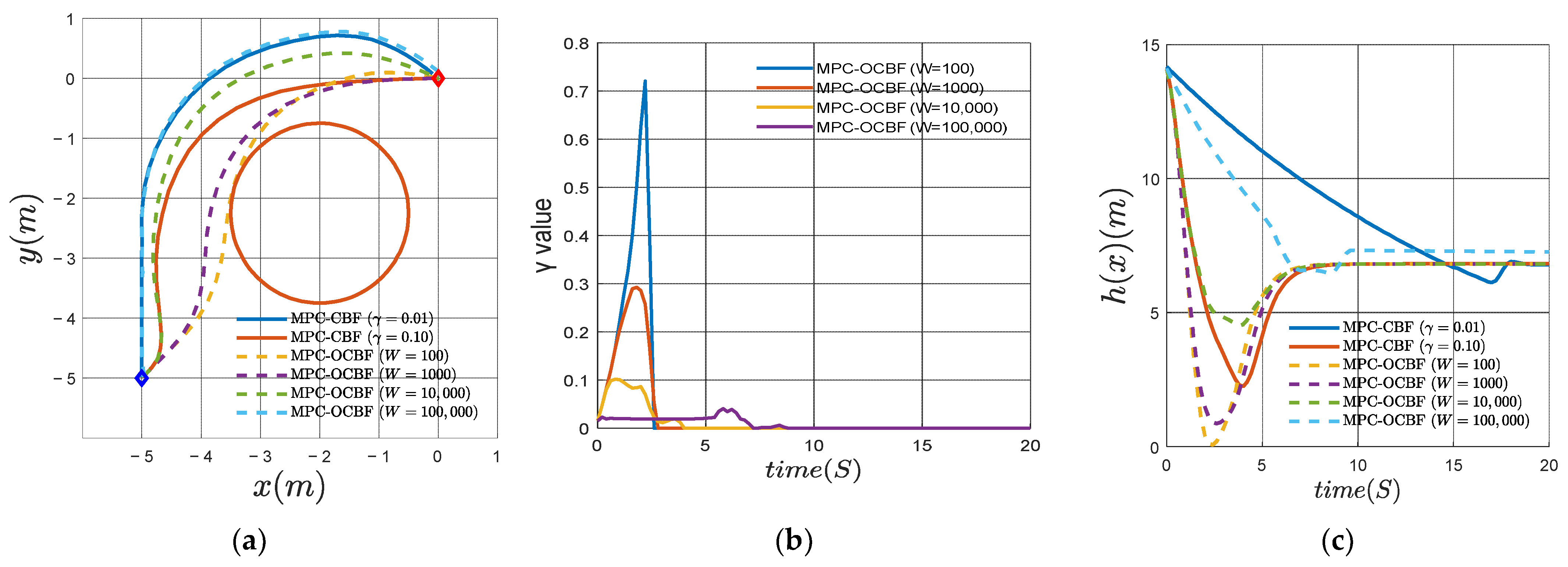
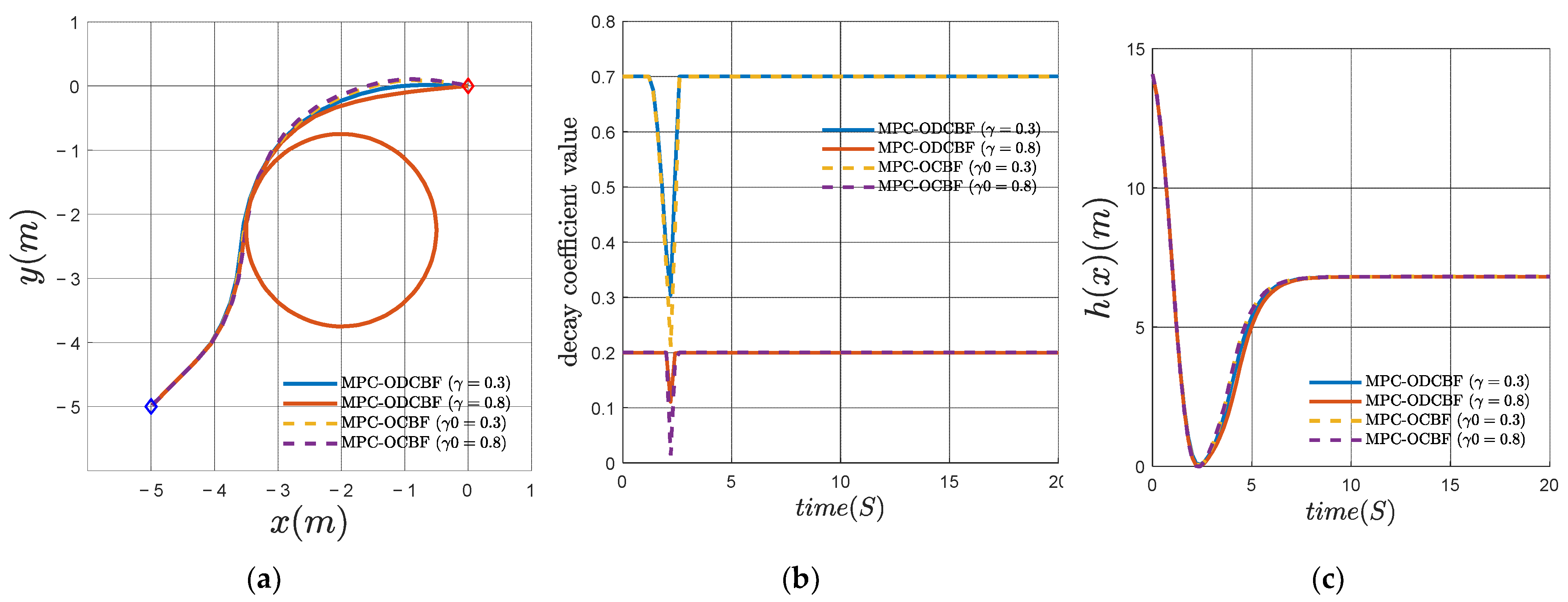
5.1. Two-Dimensional Double Integrator for Static Obstacle Avoidance
- (1)
- Prefer more conservative behaviors
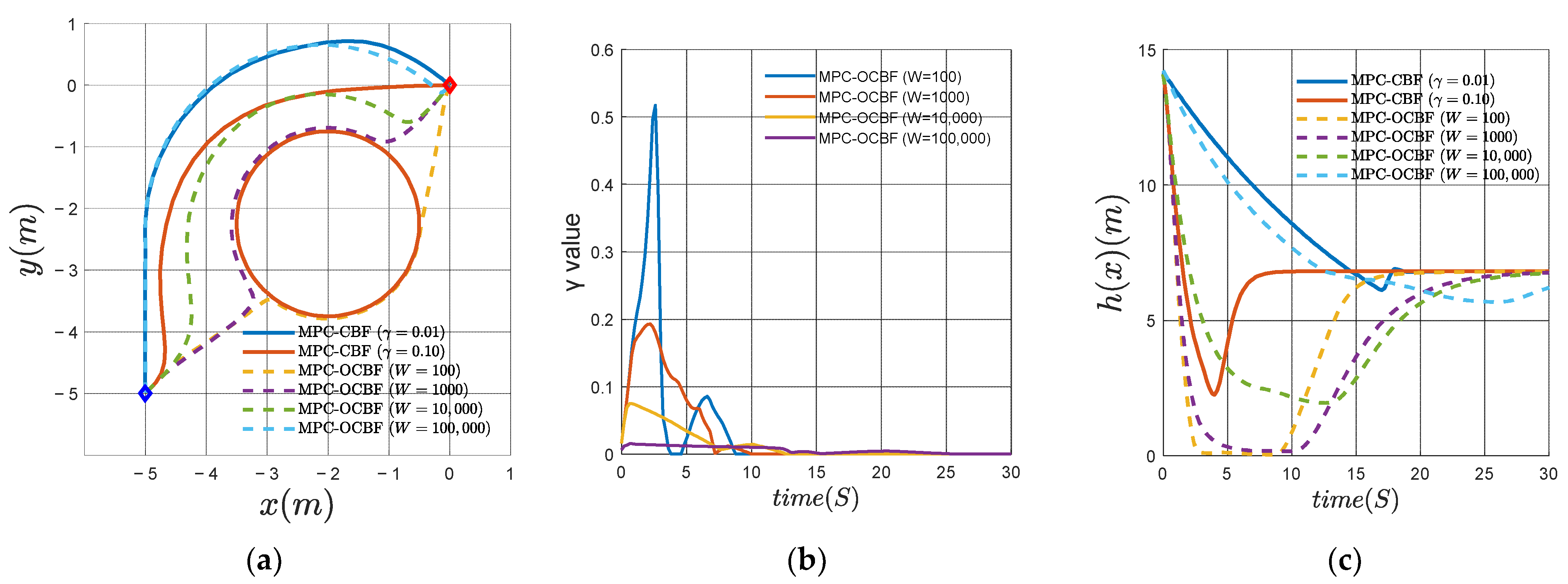
- (2)
- Prefer more aggressive behaviors
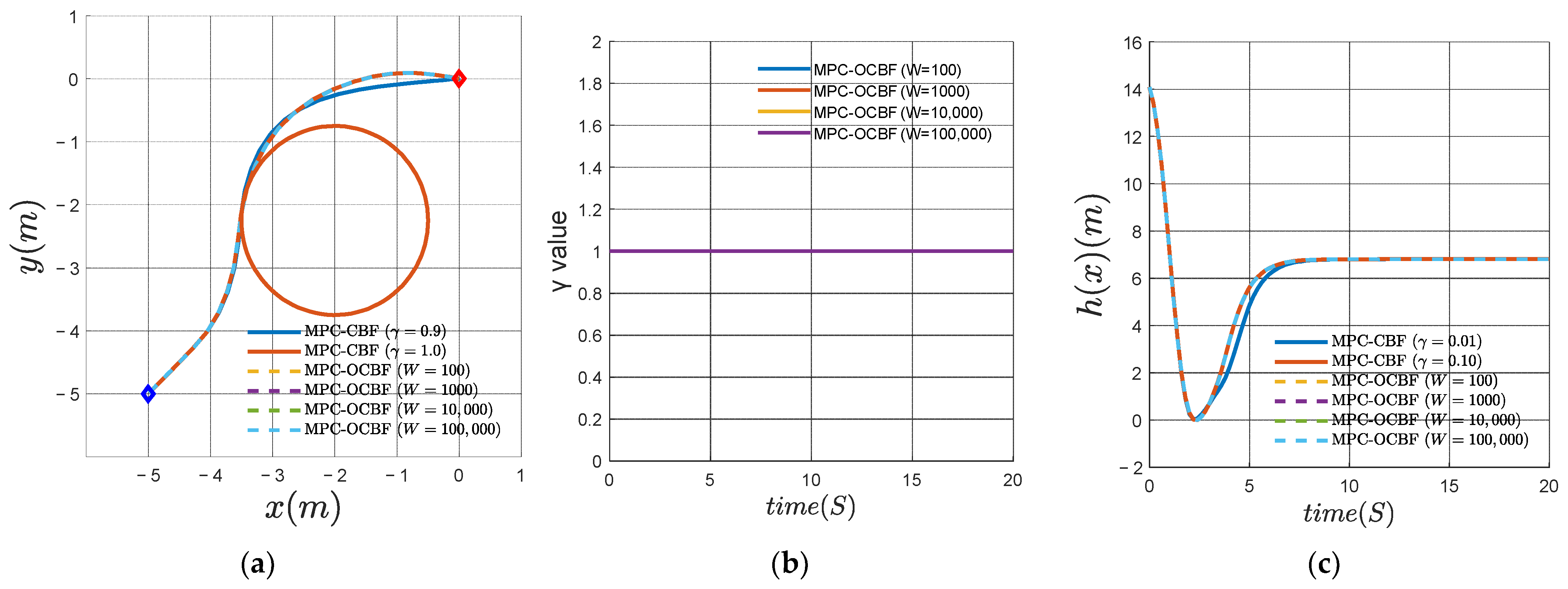
- (3)
- Prefer user-defined behaviors
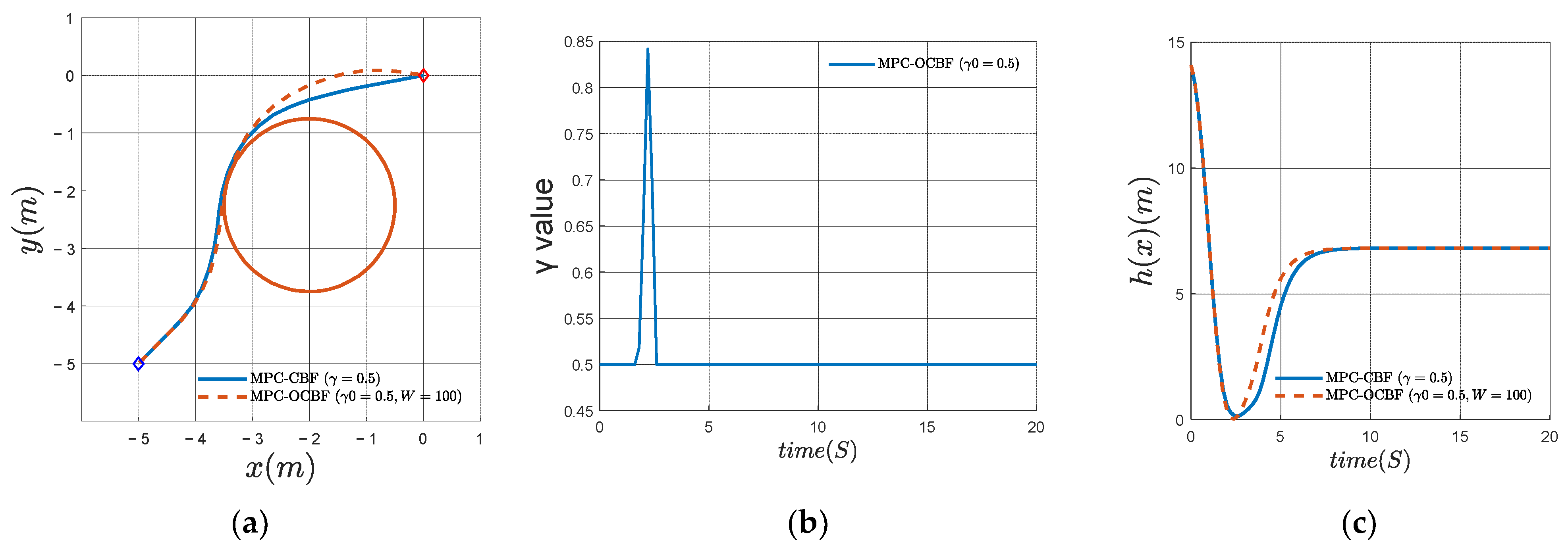
- (4)
- Compare MPC-OCBF and MPC-ODCBF with user-defined behaviors
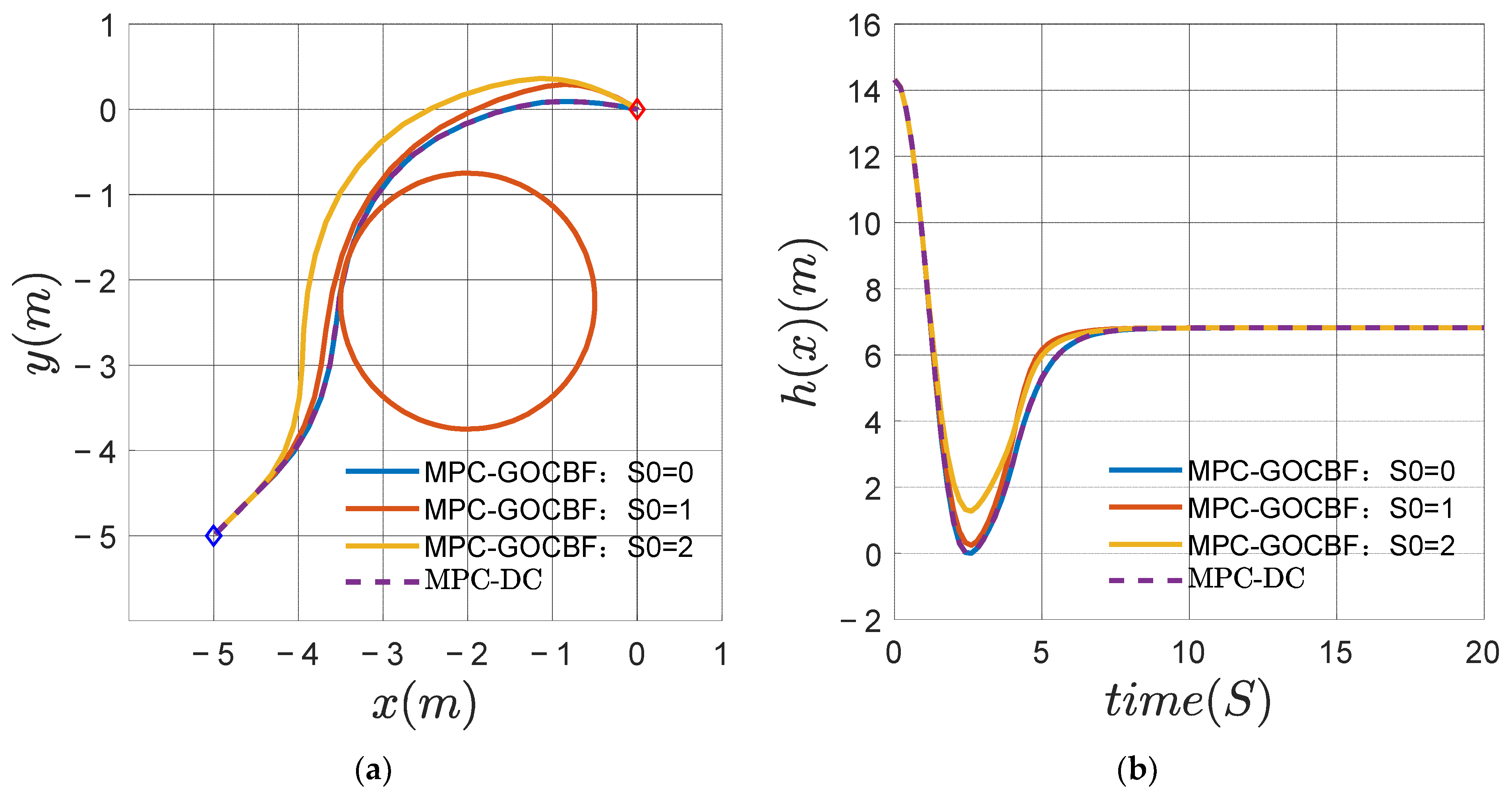
- (5)
- Compare MPC-DC with MPC-GOCBF
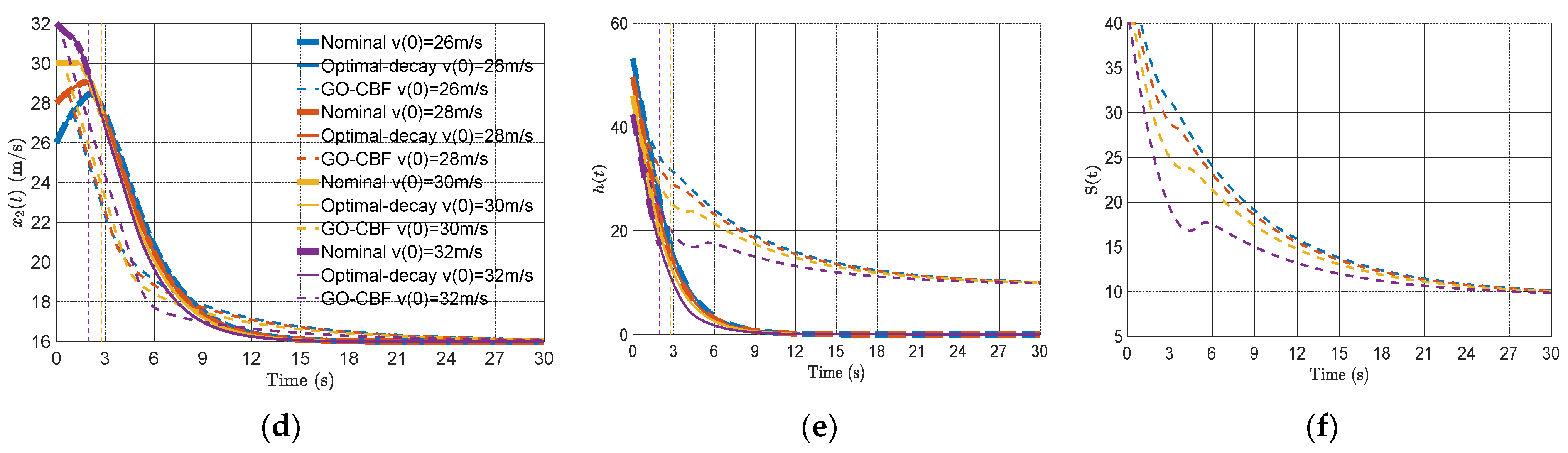
5.2. Feasibility Region Test
- (1)
- Different initial states for the discrete-time simulation
- (2)
- Different initial states for continuous simulation
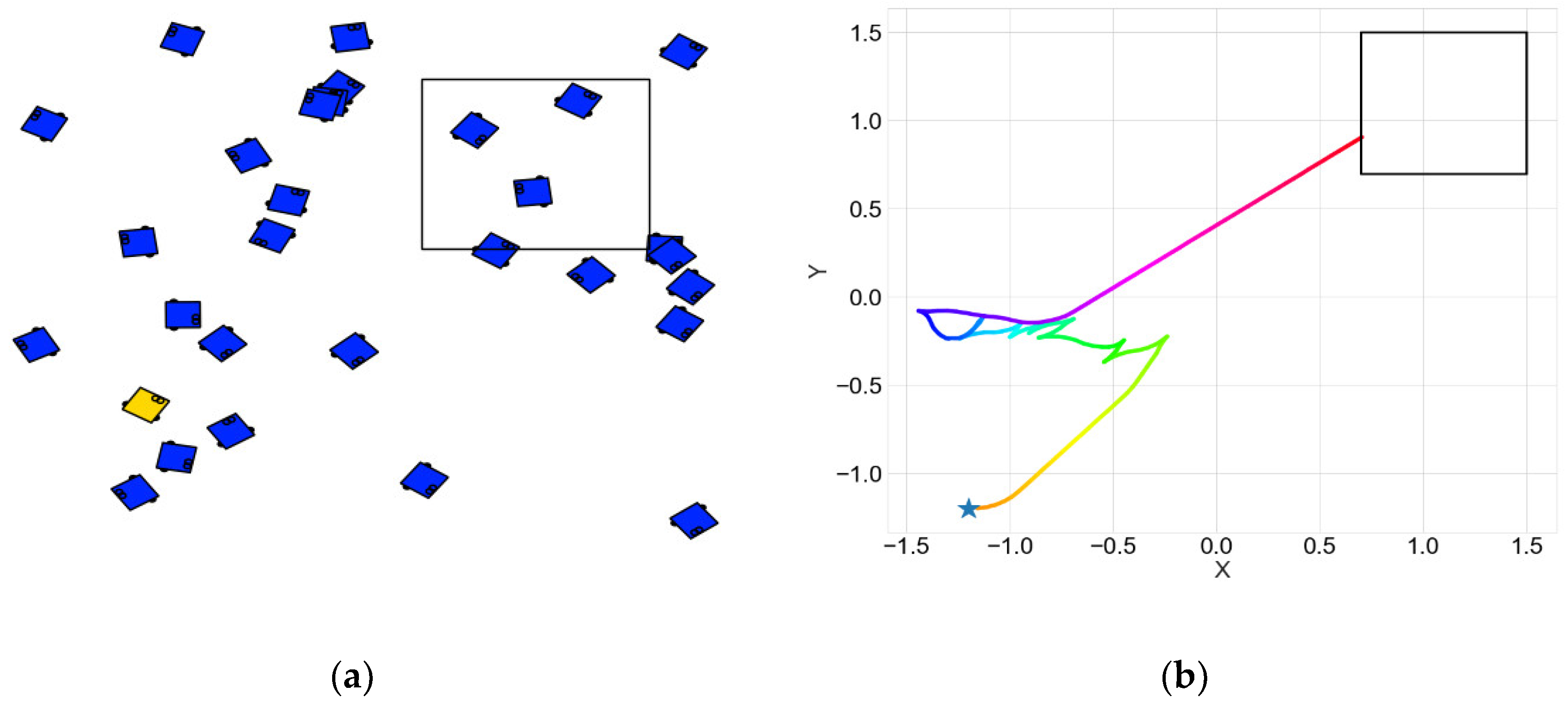
5.3. Collision Avoidance among Multi-Agents
6. Conclusions
Author Contributions
Funding
Acknowledgments
Conflicts of Interest
References
- Camacho, E.F.; Bordons, C. Model Predictive Control; Springer: London, UK, 2007. [Google Scholar]
- Wieland, P.; Allgöwer, F. Constructive safety using control barrier functions. IFAC Proc. Vol. 2007, 40, 462–467. [Google Scholar] [CrossRef]
- Ames, A.D.; Coogan, S.; Egerstedt, M.; Notomista, G.; Sreenath, K.; Tabuada, P. Control barrier functions: Theory and applications. In Proceedings of the 2019 18th European control conference (ECC), Naples, Italy, 25–28 June 2019; pp. 3420–3431. [Google Scholar] [CrossRef] [Green Version]
- Zeng, J.; Li, Z.; Sreenath, K. Enhancing Feasibility and Safety of Nonlinear Model Predictive Control with Discrete-Time Control Barrier Functions. In Proceedings of the 2021 60th IEEE Conference on Decision and Control (CDC), Virtual, 14–17 December 2021; pp. 6137–6144. [Google Scholar] [CrossRef]
- Zeng, J.; Zhang, B.; Li, Z.; Sreenath, K. Safety-Critical Control using Optimal-decay Control Barrier Function with Guaranteed Point-wise Feasibility. In Proceedings of the 2021 American Control Conference (ACC), Virtual, 25–28 May 2021; pp. 3856–3863. [Google Scholar] [CrossRef]
- Tee, K.P.; Ge, S.S.; Tay, E.H. Barrier Lyapunov functions for the control of output-constrained nonlinear systems. Automatica 2009, 45, 918–927. [Google Scholar] [CrossRef]
- Prajna, S.; Jadbabaie, A.; Pappas, G.J. A framework for worst-case and stochastic safety verification using barrier certificates. IEEE Trans. Autom. Control 2007, 52, 1415–1428. [Google Scholar] [CrossRef] [Green Version]
- Palomar, D.P.; Eldar, Y.C. Convex Optimization in Signal Processing and Communications; Cambridge University Press: Cambridge, UK, 2010. [Google Scholar]
- Aubin, J.-P. Viability Theorems for Ordinary and Stochastic Differential Equations. In Viability Theory; Springer: Berlin/Heidelberg, Germany, 2009; pp. 19–52. [Google Scholar] [CrossRef]
- Liu, J. Converse Barrier Functions via Lyapunov Functions. IEEE Trans. Autom. Control 2022, 67, 497–503. [Google Scholar] [CrossRef]
- Wisniewski, R.; Sloth, C. Converse barrier certificate theorems. IEEE Trans. Autom. Control 2015, 61, 1356–1361. [Google Scholar] [CrossRef]
- Panagou, D.; Stipanovič, D.M.; Voulgaris, P.G. Multi-objective control for multi-agent systems using Lyapunov-like barrier functions. In Proceedings of the 52nd IEEE Conference on Decision and Control, Florence, Italy, 10–13 December 2013; pp. 1478–1483. [Google Scholar] [CrossRef]
- Ames, A.D.; Xu, X.; Grizzle, J.W.; Tabuada, P. Control barrier function based quadratic programs for safety critical systems. IEEE Trans. Autom. Control 2016, 62, 3861–3876. [Google Scholar] [CrossRef]
- Mitchell, I.M.; Bayen, A.M.; Tomlin, C.J. A time-dependent Hamilton-Jacobi formulation of reachable sets for continuous dynamic games. IEEE Trans. Autom. Control 2005, 50, 947–957. [Google Scholar] [CrossRef] [Green Version]
- Asarin, E.; Dang, T.; Frehse, G.; Girard, A.; Le Guernic, C.; Maler, O. Recent progress in continuous and hybrid reachability analysis. In Proceedings of the 2006 IEEE Conference on Computer Aided Control System Design, Munich, Germany, 4–6 October 2006; pp. 1582–1587. [Google Scholar] [CrossRef]
- Althoff, M.; Grebenyuk, D.; Kochdumper, N. Implementation of Taylor models in CORA 2018. In Proceedings of the 5th International Workshop on Applied Verification for Continuous and Hybrid Systems, Oxford, UK, 13 July 2018. [Google Scholar] [CrossRef] [Green Version]
- Sontag, E.D. A Lyapunov-like characterization of asymptotic controllability. SIAM J. Control Optim. 1983, 21, 462–471. [Google Scholar] [CrossRef] [Green Version]
- Artstein, Z. Stabilization with relaxed controls. Nonlinear Anal. Theory Methods Appl. 1983, 7, 1163–1173. [Google Scholar] [CrossRef]
- Ames, A.D.; Galloway, K.; Grizzle, J.W. Control lyapunov functions and hybrid zero dynamics. In Proceedings of the 2012 IEEE 51st IEEE Conference on Decision and Control (CDC), Maui, HI, USA, 10–13 December 2012; pp. 6837–6842. [Google Scholar] [CrossRef] [Green Version]
- Agrawal, A.; Sreenath, K. Discrete Control Barrier Functions for Safety-Critical Control of Discrete Systems with Application to Bipedal Robot Navigation. In Proceedings of the Robotics: Science and Systems, Cambridge, MA, USA, 12–16 July 2017. [Google Scholar] [CrossRef]
- Son, T.D.; Nguyen, Q. Safety-critical control for non-affine nonlinear systems with application on autonomous vehicle. In Proceedings of the 2019 IEEE 58th Conference on Decision and Control (CDC), Nice, France, 11–13 December 2019; pp. 7623–7628. [Google Scholar] [CrossRef]
- Rosolia, U.; Ames, A.D. Multi-rate control design leveraging control barrier functions and model predictive control policies. IEEE Contr. Syst. Lett. 2020, 5, 1007–1012. [Google Scholar] [CrossRef]
- Rosolia, U.; Singletary, A.; Ames, A.D. Unified Multi-Rate Control: From Low-Level Actuation to High-Level Planning. IEEE Trans. Autom. Control 2022. Early Access. [Google Scholar] [CrossRef]
- Yoon, Y.; Shin, J.; Kim, H.J.; Park, Y.; Sastry, S. Model-predictive active steering and obstacle avoidance for autonomous ground vehicles. Control. Eng. Pract. 2009, 17, 741–750. [Google Scholar] [CrossRef]
- Frasch, J.V.; Gray, A.; Zanon, M.; Ferreau, H.J.; Sager, S.; Borrelli, F.; Diehl, M. An auto-generated nonlinear MPC algorithm for real-time obstacle avoidance of ground vehicles. In Proceedings of the 2013 European Control Conference (ECC), Zurich, Switzerland, 17–19 July 2013; pp. 4136–4141. [Google Scholar] [CrossRef]
- Turri, V.; Carvalho, A.; Tseng, H.E.; Johansson, K.H.; Borrelli, F. Linear model predictive control for lane keeping and obstacle avoidance on low curvature roads. In Proceedings of the 16th International IEEE Conference on Intelligent Transportation Systems (ITSC 2013), The Hague, The Netherlands, 6–9 October 2013; pp. 378–383. [Google Scholar] [CrossRef] [Green Version]
- Rosolia, U.; De Bruyne, S.; Alleyne, A.G. Autonomous vehicle control: A nonconvex approach for obstacle avoidance. IEEE Trans. Control Syst. Technol. 2016, 25, 469–484. [Google Scholar] [CrossRef]
- Zhang, X.; Liniger, A.; Borrelli, F. Optimization-based collision avoidance. Trans. Control Syst. Technol. 2021, 29, 972–983. [Google Scholar] [CrossRef] [Green Version]
- Brito, B.; Floor, B.; Ferranti, L.; Alonso-Mora, J. Model predictive contouring control for collision avoidance in unstructured dynamic environments. IEEE Robot. Autom. Lett. 2019, 4, 4459–4466. [Google Scholar] [CrossRef]
- Zeng, J.; Zhang, B.; Sreenath, K. Safety-critical model predictive control with discrete-time control barrier function. In Proceedings of the 2021 American Control Conference (ACC), New Orleans, LA, USA, 26–28 May 2021; pp. 3882–3889. [Google Scholar] [CrossRef]
- Ma, H.; Zhang, X.; Li, S.E.; Lin, Z.; Lyu, Y.; Zheng, S. Feasibility enhancement of constrained receding horizon control using generalized control barrier function. In Proceedings of the 2021 4th IEEE International Conference on Industrial Cyber-Physical Systems (ICPS), Victoria, BC, Canada, 10–12 May 2021; pp. 551–557. [Google Scholar] [CrossRef]
- Xiao, W.; Belta, C. Control barrier functions for systems with high relative degree. In Proceedings of the 2019 IEEE 58th Conference on Decision and Control (CDC), Nice, France, 11–13 December 2019; pp. 474–479. [Google Scholar] [CrossRef]
- Nguyen, Q.; Sreenath, K. Exponential control barrier functions for enforcing high relative-degree safety-critical constraints. In Proceedings of the 2016 American Control Conference (ACC), Boston, MA, USA, 6–8 July 2016; pp. 322–328. [Google Scholar] [CrossRef]
- Taylor, A.J.; Ames, A.D. Adaptive safety with control barrier functions. In Proceedings of the 2020 American Control Conference (ACC), Denver, CO, USA, 1–3 July 2020; pp. 1399–1405. [Google Scholar] [CrossRef]
- Lopez, B.T.; Slotine, J.-J.E.; How, J.P. Robust adaptive control barrier functions: An adaptive and data-driven approach to safety. IEEE Control Syst. Lett 2020, 5, 1031–1036. [Google Scholar] [CrossRef]
- Xiao, W.; Belta, C.; Cassandras, C.G. Adaptive control barrier functions. IEEE Trans. Autom. Control 2022, 67, 2267–2281. [Google Scholar] [CrossRef]
- Fan, D.D.; Nguyen, J.; Thakker, R.; Alatur, N.; Agha-mohammadi, A.-a; Theodorou, E.A. Bayesian learning-based adaptive control for safety critical systems. In Proceedings of the 2020 IEEE International Conference on Robotics and Automation (ICRA), Paris, France, 31 May–31 August 2020; pp. 4093–4099. [Google Scholar] [CrossRef]
- Khojasteh, M.J.; Dhiman, V.; Franceschetti, M.; Atanasov, N. Probabilistic safety constraints for learned high relative degree system dynamics. In Proceedings of the Learning for Dynamics and Control, Virtual, 10–11 June 2020; pp. 781–792. [Google Scholar]
- Choi, J.; Castañeda, F.; Tomlin, C.; Sreenath, K. Reinforcement Learning for Safety-Critical Control under Model Uncertainty, using Control Lyapunov Functions and Control Barrier Functions. In Proceedings of the Robotics: Science and Systems, Corvalis, OR, USA, 12–16 July 2020. [Google Scholar]
- Taylor, A.; Singletary, A.; Yue, Y.; Ames, A. Learning for safety-critical control with control barrier functions. In Proceedings of the Learning for Dynamics and Control, Virtual, 10–11 June 2020; pp. 708–717. [Google Scholar]
- Robey, A.; Hu, H.; Lindemann, L.; Zhang, H.; Dimarogonas, D.V.; Tu, S.; Matni, N. Learning control barrier functions from expert demonstrations. In Proceedings of the 2020 59th IEEE Conference on Decision and Control (CDC), Jeju, Korea, 14–18 December 2020; pp. 3717–3724. [Google Scholar] [CrossRef]
- Lofberg, J. YALMIP: A toolbox for modeling and optimization in MATLAB. In Proceedings of the 2004 IEEE International Conference on Robotics and Automation, Taipei, Taiwan, 2–4 September 2004; pp. 284–289. [Google Scholar] [CrossRef]
- Wächter, A.; Biegler, L.T. On the implementation of an interior-point filter line-search algorithm for large-scale nonlinear programming. Math. Program 2006, 106, 25–57. [Google Scholar] [CrossRef]
- Takieldeen, A.E.; El-kenawy, E.M.; Hadwan, M.; Zaki, R.M. Dipper Throated Optimization Algorithm for Unconstrained Function and Feature Selection. Comput. Mater. Contin. 2022, 1, 1465–1481. [Google Scholar] [CrossRef]
- El-kenawy, E.-S.M.; Albalawi, F.; Ward, S.A.; Ghoneim, S.S.M.; Eid, M.M.; Abdelhamid, A.A.; Bailek, N.; Ibrahim, A. Feature Selection and Classification of Transformer Faults Based on Novel Meta-Heuristic Algorithm. Mathematics 2022, 10, 3144. [Google Scholar] [CrossRef]


| Metric | Method | 20 | 30 | 40 | 50 |
|---|---|---|---|---|---|
| Success Rate | 60% | 58% | 54% | 47% | |
| 96% | 89% | 78% | 82% | ||
| MPC-GOCBF S0 = 0.01 | 98% | 97% | 94% | 85% | |
| MPC-GOCBF S0 = 0.05 | 96% | 92% | 91% | 89% | |
| Average Time | 87.85/33.36 | 96.43/37.62 | 109.93/28.44 | 114.51/31.54 | |
| 104.24/43.38 | 115.06/37.61 | 138.38/52.39 | 138.61/40.42 | ||
| MPC-GOCBF S0 = 0.01 | 102.31/41.34 | 116.55/40.63 | 120.87/36.10 | 139.36/37.74 | |
| MPC-GOCBF S0 = 0.05 | 93.88/41.31 | 113.97/39.38 | 123.69/36.66 | 133.39/1.04 | |
| Average Distance | 3.62/1.19 | 3.76/1.26 | 4.16/1.00 | 4.09/0.90 | |
| 4.13/1.64 | 4.45/1.40 | 5.12/1.97 | 4.83/1.35 | ||
| MPC-GOCBF S0 = 0.01 | 3.99/1.48 | 4.34/1.32 | 4.46/1.22 | 4.83/1.25 | |
| MPC-GOCBF S0 = 0.05 | 3.75/1.39 | 4.25/1.35 | 4.45/1.34 | 4.55/1.04 |
| N = 20 | ||||||
|---|---|---|---|---|---|---|
| Source of Variance | SS | DF | MS | F (DFn, DFd) | p-value | F crit |
| Between Group | 13,368.813 | 3 | 4456.271 | 2.694 | 0.046 | 2.631 |
| Within Group | 572,304.456 | 346 | 1654.059 | |||
| Total | 585,673.267 | 349 | ||||
| N = 30 | ||||||
| Source of Variance | SS | DF | MS | F (DFn, DFd) | p-value | F crit |
| Between Group | 17,250.872 | 3 | 5750.291 | 3.782 | 0.011 | 2.631 |
| Within Group | 504,757.887 | 332 | 1520.355 | |||
| Total | 522,008.759 | 335 | ||||
| N = 40 | ||||||
| Source of Variance | SS | DF | MS | F (DFn, DFd) | p-value | F crit |
| Between Group | 27,758.935 | 3 | 9252.978 | 5.834 | 0.000688 | 2.633 |
| Within Group | 496,406.018 | 313 | 1585.962 | |||
| Total | 524,164.953 | 316 | ||||
| N = 50 | ||||||
| Source of Variance | SS | DF | MS | F (DFn, DFd) | p-value | F crit |
| Between Group | 22,012.770 | 3 | 7337.590 | 5.746 | 0.000781 | 2.635 |
| Within Group | 381,796.187 | 299 | 1276.910 | |||
| Total | 403,808.957 | 302 | ||||
| N = 20 | ||||||
|---|---|---|---|---|---|---|
| Source of Variance | SS | DF | MS | F (DFn, DFd) | p-value | F crit |
| Between Group | 12.923 | 3 | 4.308 | 2.034 | 0.109 | 2.631 |
| Within Group | 732.641 | 346 | 2.117 | |||
| Total | 745.564 | 349 | ||||
| N = 30 | ||||||
| Source of Variance | SS | DF | MS | F (DFn, DFd) | p-value | F crit |
| Between Group | 18.325 | 3 | 6.108 | 3.417 | 0.0177 | 2.632 |
| Within Group | 593.547 | 332 | 1.788 | |||
| Total | 611.872 | 335 | ||||
| N = 40 | ||||||
| Source of Variance | SS | DF | MS | F (DFn, DFd) | p-value | F crit |
| Between Group | 35.344 | 3 | 11.781 | 5.640 | 0.000893 | 2.633 |
| Within Group | 653.783 | 313 | 2.089 | |||
| Total | 689.126 | 316 | ||||
| N = 50 | ||||||
| Source of Variance | SS | DF | MS | F (DFn, DFd) | p-value | F crit |
| Between Group | 20.837 | 3 | 6.946 | 5.034 | 0.00203 | 2.635 |
| Within Group | 412.517 | 299 | 1.380 | |||
| Total | 433.355 | 302 | ||||
Publisher’s Note: MDPI stays neutral with regard to jurisdictional claims in published maps and institutional affiliations. |
© 2022 by the authors. Licensee MDPI, Basel, Switzerland. This article is an open access article distributed under the terms and conditions of the Creative Commons Attribution (CC BY) license (https://creativecommons.org/licenses/by/4.0/).
Share and Cite
Li, S.; Yuan, Z.; Chen, Y.; Luo, F.; Yang, Z.; Ye, Q.; Fu, W.; Fu, Y. Optimizable Control Barrier Functions to Improve Feasibility and Add Behavior Diversity while Ensuring Safety. Electronics 2022, 11, 3657. https://doi.org/10.3390/electronics11223657
Li S, Yuan Z, Chen Y, Luo F, Yang Z, Ye Q, Fu W, Fu Y. Optimizable Control Barrier Functions to Improve Feasibility and Add Behavior Diversity while Ensuring Safety. Electronics. 2022; 11(22):3657. https://doi.org/10.3390/electronics11223657
Chicago/Turabian StyleLi, Shilei, Zhimin Yuan, Yun Chen, Fang Luo, Zhichao Yang, Qing Ye, Wei Fu, and Yu Fu. 2022. "Optimizable Control Barrier Functions to Improve Feasibility and Add Behavior Diversity while Ensuring Safety" Electronics 11, no. 22: 3657. https://doi.org/10.3390/electronics11223657