1. Introduction
Most people living in modern civilization are provided with electricity produced by the state or private enterprise. From the perspective of the private company or government that supplies electricity, it is important to manage electric power received so that it can be used efficiently. From the perspective of providing electricity, it is necessary to understand how customers use the electric power they receive to make plans to reduce various costs in terms of production and supply [
1,
2]. Therefore, analyzing data on how customers use electric power has become an important task for most electric power providers [
3].
In general, data representing the electric power used by customers are stored and recorded in a time series [
4,
5]. This is because the detector recodes electric power usage according to the time unit. These data obtained through this process have various features, such as cycles and trends over time. However, detection devices for calculating the electric power used by customers can lose data uniformity due to various environmental factors. Considering possible electric power system component failures, communication failures, protection failures, and market and load uncertainties, it is important to analyze recorded power data by taking errors resulting from various factors into account [
6,
7,
8].
Detection of anomalies in power usage data is a task that can monitor whether power is wasted. Most power usage data take the form of time series data. The usage is recorded according to the unit of time, and they are gathered to show one periodic characteristic. In these cases, anomalies are measured using a variety of statistical techniques [
9,
10] or simple LSTM-AE family models [
11,
12,
13]. However, if it is not a point anomaly in which anomalies are recorded in only a single time unit, but a collective anomaly in which anomalies are accumulated over a day or more, the effect of statistical techniques is not greater than before. Since power usage data have periodicity, context should also be considered when it comes to anomalies. So, most anomalies in power usage data have contextual properties. The contextual anomaly has many variables to refer to and it is difficult to know which variables to refer to. Therefore, it is worthwhile to try different conditions and methodologies to detect anomalies in power usage data [
14,
15,
16].
In addition, since electric power detection devices are provided to individuals, data belonging to a cluster corresponding to a unit (building, apartment complex, region) are not subjected to the same environmental change, making it difficult to cluster. If common environmental variables are applied in clusters, data features can be easily extracted by using a single method of clustering. However, since data with various errors are combined and delivered, it is important to cluster data to which individual environmental variables are applied. Studies have been conducted using various clustering methods or using clustering with complex process forms [
17], such as clustering data from electrical power distribution systems using a feature-based clustering approach that performs principal component analysis first [
18]. By using a clustering method to detect anomalies in power usage data, capturing features of recorded data according to environmental variables can be advanced.
To detect anomalies in the power usage time series data recorded according to various environmental variables, a pre-clustering method can be used in the data preprocessing step, and various methods other than the anomaly detection method using the existing LSTM and statistical techniques can be used. In this paper, we used a CNN-based binary classification model that is different from existing methods to preprocess time series data with various pre-clustering methods and to detect effective anomalies. To apply the CNN-based model to time series data, methods for generating time series images were applied. If the approach proposed in this paper is used, we can show high performance in electric power analysis tasks such as anomaly detection of power data in various electric power detection systems. For example, in a smart grid, a pre-clustering-based power anomaly detection method can be used to have a generation-optimized electric power supply pattern. Moreover, the method of this study can be adapted to label the generation in which anomalies are recorded.
The rest of this paper is organized as follows.
Section 2 introduces time series data, an important keyword appearing in this paper, the clustering method used in this experiment, and methods for generating time series images.
Section 3 shows the overall clustering process and anomaly detection method used in the experiment. Experimental results and conclusions are summarized in
Section 4 and
Section 5, respectively.
2. Related Research
This section introduces the algorithms and concepts mentioned and used in this study. How electric power data are collected and pre-processed, general-purpose clustering algorithms for time series data, and generating time series image algorithms used in this study are described in this section.
2.1. Electric Power Data
Large-scale electric power suppliers provide power systems to private customers, supply current separately, and provide services in the form of receiving cost for the usage. Providers generate electric power through power plants, build facilities to supply power to customers, sell power to customers, and record calculated data. Electric power data are classified into three categories according to the place and time when data are recorded. The first is power generation statistics, which record the amount of power produced by power plants. The second is facility statistics, which show the trends and status of facilities built to supply power to private users. The third is sales statistics, which supply power to users and record how much power they lose during supply.
Power data are preprocessed from raw data into various types of data. Image data are used for visually expressing power facilities, faults, or defects. For example, we can use a picture of a detector or a faulty power plant equipment as image data. Financial data are used for expressing financial characteristics such as unit price and monthly sales volume to establish a supply plan. Financial data include data that adjust unit price to plan power supply according to the recorded amount of electric power. Time series data are used for recording data in which private customers use power over time or receive power from power plants. Time series data can be used to perform a variety of tasks, such as making predictions and detecting anomalies [
19]. In general, data such as power supply and demand, power demand, and power loss are used to predict the power consumption of private customers and to cluster power demand patterns. Since all data are recorded and collected over time, time series data are the basic type of electric power data because it is easy to preprocess such data. Power suppliers need to understand features of electric power data by clustering collected data to efficiently establish power supply and facility maintenance plans.
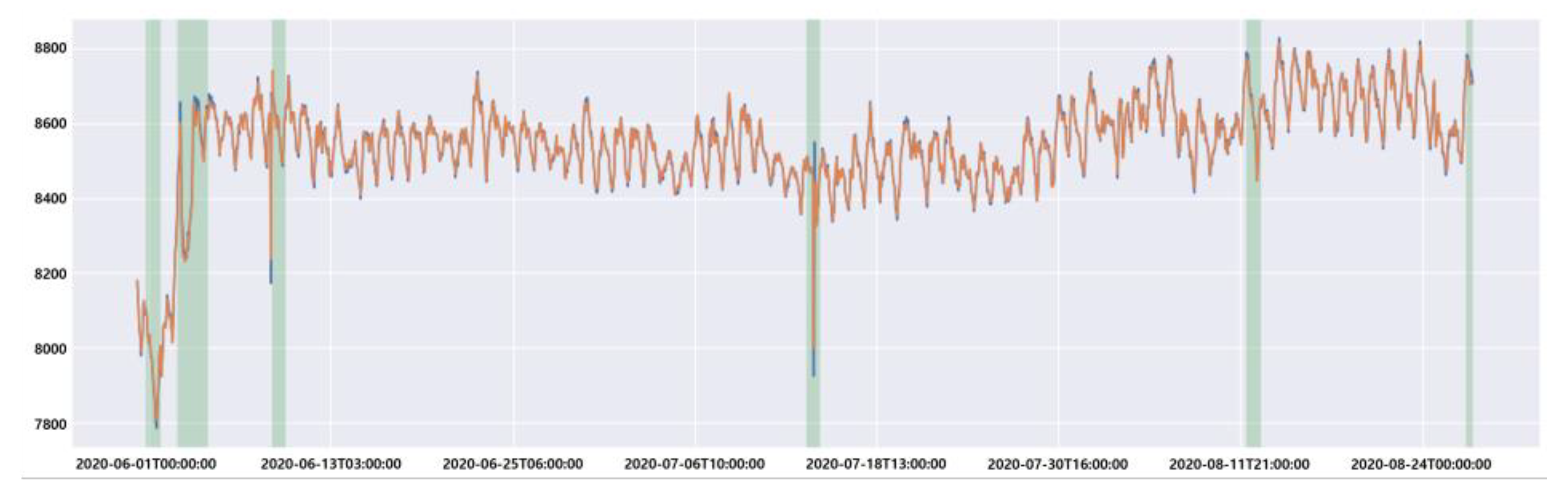
Figure 1 is an example of normalized power data actually detected in a building. We can clearly see the trend in electric power usage from day to day, and if we take a long time unit as a basis, we can see the trend in that electric power usage. These data are recorded by a general building detector, and if the detector malfunctions due to various environmental factors, the maximum or minimum value of the measured power value may be recorded abnormally.
2.2. Time Series Data Clustering
The goal of clustering is to identify structure in an unlabeled dataset by objectively organizing data into homogeneous groups where the within-group-object similarity is minimized, and the between-group-object dissimilarity is maximized. Unlike static data, which have certain rules and fixed format, time series data have a feature in that values will change with time. Given a set of unlabeled time series, it is often desirable to determine groups with similar time series.
Figure 2 shows three different approaches: raw-data-based, feature-based, and model-based. Note that the left branch of the model-based approach trains the model and uses model parameters for clustering without needing another clustering algorithm. Unlike a raw-data-based approach, a feature-based approach has steps to extract features, allowing researchers to effectively understand characteristics of the data. A model-based approach clusters by extracting model parameters or determining coefficients and residuals through various models. This approach allows researchers to proceed with the clustering process and use several general-purpose clustering algorithms to cluster according to the given data [
20,
21,
22].
2.2.1. Agglomerative Hierarchical Clustering
An agglomerative clustering method can repeatedly perform the following commands. At startup, each data coordinate is designated as one cluster and two most similar clusters are merged. At that time, similar clusters are combined until the specified number of clusters remains. There are three main ways to merge two clusters. The first is Ward, which merges two clusters so that the increase of variance within all clusters is the smallest. The second is average, which combines two clusters with the shortest average distance between cluster centers. The third is complete, which combines two clusters with the shortest maximum distance between cluster points.
Cluster aggregations each stage or level are grouped into cluster trees and operated, forming a layer of trees. As shown in
Figure 3 below, agglomerative or divisive strategies are performed depending upon whether a bottom-up or top-down strategy is used. The agglomerative hierarchical clustering method is more popular than the divisive method. Hierarchical clustering is not restricted to cluster time series with equal length. It is applicable to series of unequal length as well if an appropriate distance measure such as DTW (dynamic time warping) is used to compute similarity.
2.2.2. K-Means and Fuzzy c-Means
K-means (interchangeably called c-means in this study) was first developed more than three decades ago. The main idea behind it is the minimization of an objective function, which is normally chosen to be the total distance between all patterns from their respective cluster centers [
23,
24,
25]. The centroid is randomly determined by the initial value of k. After that, the process of touring all data is repeated to assign each dataset to the cluster to which the nearest centroid belongs. The centroid then moves to the center of the cluster. Algorithms alternate until the value of the objective function can no longer be reduced.
Given
patterns
, c-means determine
cluster centers
, by minimizing the objective function given as:
where
in the above equation is normally the Euclidean distance measure. However, other distance measurements can also be used. Recurring solution procedures typically have the following steps:
Choose and (number for stopping the iterative procedure). Set the counter and the initial cluster center, , arbitrarily.
Distribute to determine such that is minimized. This is achieved normally by reassigning to a new cluster that is closest to it.
Modify cluster centers .
Stop if the change in is smaller than ; otherwise, increment and repeat steps 2–3.
Dunn has devised a method using fuzzy segmentation by expanding the k-means algorithm and presenting the objective function as shown in Equation (2) below [
26,
27]:
Note that
in this equation and the following equations denotes the matrix of a fuzzy c-partition (same as k-partition). Fuzzy c-partition constraints are conditions under the objective function of Equation (2). In other words, each
could belong to more than one cluster with each belongingness taking a fractional value between 0 and 1. Bezdek has generalized
to an infinite number of objective functions. The new objective function subject to the same fuzzy c-partition constraints is shown in Equation (3) below:
By specifying the number of clusters and weighting coefficient, alternative optimization procedures are repeated to solve the fuzzy c-means model. The fuzzy c-means algorithm works better for time series with the same length. This is because the concept of the cluster center is unclear when the same cluster contains different time series of different lengths [
28,
29,
30]. Various methods using fuzzy and k-means algorithms have been applied and developed for clustering [
31,
32,
33].
2.2.3. Self-Organizing Maps (SOM)
Self-organizing maps developed by Kohonen [
34] are a type of neural network in which neurons are arranged in a low-dimensional structure and trained by repetitive unsupervised learning or self-organizing procedures. The weight vector of the neuron is initialized. After presenting the pattern, it is updated according to the distance between the input pattern and the weight vector. This is in accordance with the following rule:
As neighboring neurons are updated at each stage, neighboring neurons in the network tend to indicate neighboring locations in feature spaces. Like the k-means and fuzzy c-means algorithms, SOM is an inappropriate algorithm for time series whose lengths are not the same because it defines dimensions of the weight vector [
35].
In addition to methods describe above, there are various methods for clustering time series data. There is an approach that has an algorithm suitable for applying features of a time series rather than static data. However, if data are recorded with complex environmental variables such as electric power data, it is difficult to define similar time series groups and extract their characteristics. Thus, it is often desirable to learn the characteristics of time series groups using multiple clustering techniques or adopting clustering using neural network techniques. Among various neural network techniques, a method of estimating subspaces and generating sample clustering using adversarial learning effectively analyzed features and clustered data of multidimensional and multivariate data.
2.2.4. K-Shapes
The k-means algorithm classified clusters according to the homogeneity between individual observations using Euclidean distance (ED) to measure the distance between the data and the center of the cluster. Unlike that, the k-shape algorithm proposed by John Paparrizos [
36] uses a distance measurement method called CC (cross-correlation). When two data are given in the form of a sequence, if an
of padding is given in one direction, much leading occurs. Considering that the lengths of the two sequences are the same as
and the maximum case of possible readings, the lengths of the sequences are 2m − 1. Currently, the purpose of CC is to find a shifting point that gives padding by 2m − 1 and maximizes similarity when calculating ED. According to the convolution theory, CC can be defined as Equation (5).
Since fast forwarder transform (FFT) can be used to reduce the time complexity of obtaining CC, CC is defined using the above equation. Additionally, to increase performance, the k-shape algorithm normalizes CC. This is called normalized cross-correlation (NCC). The k-shape algorithm uses the objective function shown in Equation (6) below.
Since it means that the two-sequence data are close as the NCC (normalized cross-correlation) increases, the value obtained by subtracting the maximum NCC from 1 is used as the objective function. The k-shapes algorithm used CC, a distance measurement method that can be calculated from sequence data, not ED used by k-means. K-shapes show excellent performance when using sequence-type data, i.e., time series data, because they used approaches such as the dynamic time warping (DTW) method of finding points that correspond to the mean value.
2.3. Generating Time Series Images
2.3.1. Recurrence Plot (RP)
The recurrence plot algorithm is a visualization algorithm that aims to explore the m-dimensional phase space trajectory by expressing the regression of data values in two dimensions [
37,
38]. To convert time series data into images using RP, the m-dimensional spatial trajectory of time series data must first be configured. Given the time series data as
, the m-dimensional spatial trajectory can be defined as Equation (7) below.
sn can be seen as the trajectory of time series data from
xn to
xn+1. To express trajectory information in the form of a matrix, a distance matrix may be defined based on spatial trajectory data. To express this mathematically, the elements of the matrix can be defined as Equation (8) below.
ε is the distance threshold, and is the unit step function. is the element value of the distance matrix and means the distance (Norm) between and in the equation. Thus, the distance matrix is represented by a matrix of distances between the two s. The diagonal elements of R become zero because they define the distance from themselves. Additionally, and are the same according to the definition of Equation (2) and thus become symmetric matrices. The time series image converted by the RP algorithm describes a collection of time pairs at the same location of orbit. If that orbit is strictly periodic through period , then all pairs of times are separated by multiples of and displayed diagonally. That is, the visual representation of the RP provides information on the period and the change width of the time series data.
2.3.2. Gramian Angular Field Algorithm
A Gramian Angular Field (GAF) is an algorithm that expresses temporal correlation between each time point based on polar coordinates. Polar coordinate-based matrices have the advantage of preserving time correlations when changing time series data into images [
39]. Since the GAF may first have a given time series data value too large or too small, it is normalized to the interval
or
. The time index
of the normalized signal
is expressed in radius
, and is converted into polar coordinates as shown in Equation (9) below with the angle
.
Here,
N is the normalization constant for the range of polar coordinate systems. GF is divided into two ways depending on the sum and difference of angles. The Gramian angular summary field (
GASF) is expressed as the sum of the angles of polar coordinate time series data consisting of time pairs of
i and
j, and then is defined as Equation (10).
Gramian angular difference field (
GADF) is defined as Equation 5 of the difference between the angles of the polar coordinate system as opposed to
GASF.
GAF preserves time dependence because time increases as it moves from the top left to the bottom right. Since the main diagonal line includes the value and angle information of the raw data, the raw data may be recovered using the same.
2.3.3. Markov Transition Field Algorithm
The Markov transition field (MTF) algorithm is an algorithm representing the probability of transition of time series data that is discretized [
39]. To configure the MTF, the given time series dataset
X is divided into
Q sections according to the value, and then assigned to the interval
corresponding to the time series data value
of the time index
. In the first Markov chain method along the time axis, a weighted adjacency matrix W of the size of
is constructed as shown in Equation (12) below.
represents the frequency of transition from the
interval to the
interval. By normalizing the sum of each column of
W to 1, the Markov transition matrix can be constructed. In this process,
W eliminates the distribution of
X and the time dependence on the time index
. To overcome the information loss of
W, MTF is defined as Equation (13) below by aligning each probability along the time order.
, which is the i-row j-column value of MTF, represents the probability of transitioning from the interval
to which the data value of time index
belongs, to the interval
to which the data value of time index
belongs. That is, the probability of transition between points where the difference is between the two times k. If the width of the section is large, most of the values are counted as the section closest to the average, and if the width of the section is small, the value aggregated in the extreme section is reduced [
39].
3. Experiment
This section describes the pre-clustering and anomaly detection methods proposed in this study. After explaining the data used in the experiment in detail, the experiment process according to the clustering algorithm and anomaly detection method used in the experiment is described.
3.1. Dataset
In this study, time series power data are clustered to predict and analyze power data. The dataset used in this study is data that store power consumption provided by the Korea Energy Agency. The electric power usage of 60 buildings was recorded every hour from 1 June 2020 to 24 August 2020. The column of the dataset is configured as shown in
Table 1 below. There are a total of 122,400 rows in the dataset, and no outliers exist.
Figure 4 shows a boxplot for each column in the dataset. Outliers were recorded in the wind speed column and humidity column in all buildings, and few outliers were found in power usage or temperature. In this study, the performance of time series data prediction and analysis according to the presence or absence of clustering was compared using the above dataset. Columns other than electric power usage were not used to measure performance under the same conditions and to consider the characteristics of power data. This experiment compared the performance according to the clustering technique performed in the preprocessing process to predict the power consumption dataset in a time series data format.
3.2. Clustering Methods
In the pre-clustering step, 60 building power usage data were clustered. To detect anomalies, time series data were clustered to apply the time series feature of each cluster. For detecting an anomaly, we clustered using four methods to explore effective clustering methods. The first was to use only the power usage column. Anomaly detection was performed using only single-dimensional data without separate categorical data. Second and third, power usage data were clustered using the k-means and k-shapes algorithm and separate categorical data were added and used. To set k, clustering was performed from 1 to 60, the maximum number of buildings, and the appropriate k was set using the elbow method. As a result, it was appropriate to set k to 7 as shown in
Figure 5. The clustering results using the k-shape algorithm can be confirmed in
Figure 6. Fourth, power usage data were clustered using the SOM algorithm and separate categorical data were added and used. To determine the optimal number of nodes and map arrangement, appropriate nodes were obtained using Equation (14) proposed by Tian et al.
is the number of objects to be observed and is the number of neurons, which is an integer close to the value of the right-hand side. When the observation target is 60 (number of builds), the number of neurons calculated was about 39 ). Therefore, clustering was performed using SOM composed of a feature map of 7 × 6 corresponding to the number of arrays close to the number of neurons.
3.3. Data Preprocessing and Add Anomaly for Learning
We needed to preprocess the data to detect whether anomalies were recorded on a daily basis within a total of 60 building power usage data belonging to a certain number of clusters. For each building, the power usage data were recorded every hour for 85 days. Building power usage data were divided into 85 sections to extract daily power usage data. In conclusion, power usage data having a shape of (60, 2040) were preprocessed into data having a shape of (60, 85, 24). For example, if there were 12 building power usage data in the first cluster, these data were converted into time series data with a shape of (12, 85, 24).
Anomalies were not recorded in the dataset used in this experiment. As shown in
Figure 7, we had a process of arbitrarily injecting anomalies to construct a training model that detects anomalies through supervised learning. First, the daily power usage data were normalized. Anomalies were injected by converting any data from normalized daily power usage data to values close to the maximum and minimum values in daily data. Additionally, the index of the data with injected anomalies was extracted and set as the label to be used in supervised learning. In conclusion, anomalies were injected into random indexes, and this label was set to ground-truth and used as a y dataset for the model trained in this experiment.
3.4. Using ARIMA for Detecting Anomalies
We adopted a method using ARIMA that statistically analyze time-series data, to validate and compare the performance of imaging time-series data for anomaly detection. The optimal p, d, and q factors were searched by applying the ARIMA model to the preprocessed power usage time series data. As a result of the search, we confirmed that (p, d, q) has the most appropriate ARIMA model when (4, 1, 1). In the analyzed time series data, the date on which data having a difference value of 10 or more is recorded is defined as data on which anomalies are recorded. As shown in
Figure 8 below, after visualizing the data at the time when the anomalies were recorded, the date containing the data was anomaly defined and an F1-score was given compared to the label.
3.5. Generating Time Series Images
In this experiment, as shown in
Figure 9, time series images were generated using RP, GASF, GADF, and MTF algorithms for time series data recorded in 24 h time units. When using the RP algorithm, the cross recurrence plot generates a black and white time series image by substituting 1 if it is greater than a certain distance (element value), but in this experiment, the distance threshold was not used to obtain more information from data in the CNN model. CNN-based layers were designed as shown in
Table 2 with the generated time series image to learn a model that classifies normal data and anomalies.
Then, as shown in
Figure 10,
Figure 11,
Figure 12 and
Figure 13, time series data recorded for 85 days were imaged. Time series data recorded over 85 days per building were imaged using 85 recurrence plot (RP), GASF, GADF, and MTF algorithms. The time series image coordinate values calculated through each algorithm are expressed as
Figure 10,
Figure 11,
Figure 12 and
Figure 13 through colormap. In
Figure 11,
Figure 12 and
Figure 13, the colormap used in this figure is a jet, which set a minimum value to blue and a maximum value to red, so the coordinate values are converted into colors in RGB format in jet colormap. Exceptionally, in
Figure 10, we used a specific colormap, which set a minimum value to blue and a maximum value to yellow. Data with existing shapes (60, 85, 24) have been increased to (60, 85, 24, 24) shapes. The two results were compared using original data and dimensionally increased data as training and testing data for anomaly detection models. As ARIMA models were used to detect anomalies for each clustered time series data, CNN-based models can be used to classify whether they were anomalies by converting clustered power usage data into time series image datasets.
3.6. Using CNN-Based Model for Detecting Anomalies
Although CNN is mainly used for object (defect, forgery, etc.) detection or image analysis, in this experiment [
40,
41], a convolutional neural network was used for binary classification of image datasets generated using four algor ithms. The neural network structure for binary classification is specified in
Table 2. Since the shape of the image data used in this experiment was (24 and 24), the dimensions of the input data were set to (1, 24, 24). A neural network was constructed to determine whether the input image data were an anomaly through the neural network and to calculate a value close to 1 if normal and 0 if anomaly. After constructing two convolutional layers, a fully connected layer was placed for binary classification. The epoch was set to 50 to ensure sufficient learning. For the label for learning, the label constructed in the preprocessing stage of injecting anomaly was used, and the model was trained by dividing 70% of the training dataset and 30% of the test dataset to contain the same ratio of anomalies.
4. Result
In this experiment, the F1-score metric was used to indicate the accuracy of the model for detecting anomalies. To use a metric that shows higher accuracy, as the number of false positives and false negatives is reduced in the confusion matrix, the F1-score using the harmonic average of precision and recall was selected as the metric. Models for detecting anomalies for each cluster were separately configured and trained, and the F1-scores of the clusters were averaged and are shown in
Table 3 to evaluate the performance of each method.
As a result of the experiment, the clustering method using the SOM algorithm had the highest accuracy when pre-clustering for anomaly detection, and the accuracy was lower than the non-clustering method. In addition, after pre-clustering, the case of applying the CNN-based binary classification model by generating the time series data image obtained higher accuracy than the case of applying the ARIMA model using the time series data as it is. When the time series data image generation method was applied, the model to which the MTF algorithm was applied yielded the highest F1-score.
5. Conclusions
In this paper, we proposed a CNN-based anomaly detection model using time series images after pre-clustering to detect anomalies in time-recorded power data. In previous studies, anomalies were detected using a statistical model or an RNN-based unsupervised learning model to consider the statistical characteristics of time series data. The proposed method uses a pre-clustering technique to characterize time series data collected from various domains. In addition, to effectively detect anomalies, a CNN-based unsupervised learning model specialized for binary classification was used by converting time series data into time series image data. To use the proposed method, three methods of pre-clustering and four methods of converting time series data into images were used to compare performance.
For this experiment, data recorded and provided every hour from 1 June 2020 to 24 August 2020 were used, and data per hour were purified into data every three hours and normalized to perform clustering. The effectiveness of pre-clustering was proved by comparing the prediction accuracy according to the presence or absence of pre-clustering. In addition, other clustering techniques were compared to evaluate best pre-clustering techniques. K-means and k-shapes clustering techniques were conducted using the elbow method, and clustering was performed by setting appropriate neurons according to the number of observations to utilize SOM.
After pre-clustering, the power time series data written in this study was converted into an image form using recurrence plot, Gramian angular field, and Markov transition field algorithms, and anomaly data and normal data were discriminated using a CNN-based binary classification model. The performance of the anomaly detection model using all CNN-based time series image data were better than the performance of the anomaly detection method using the ARIMA model using the existing time series data. In particular, the performance of the binary classification model using the time series image dataset constructed using the MTF algorithm was the best.
For anomaly detection of time series data, pre-clustering the time series data and applying the anomaly detection model individually to each cluster showed higher performance than training the raw data on a single model. In addition, using a CNN-based unsupervised learning model by imaging time series data showed equivalent or better performance than using an ARIMA model using raw data. Therefore, to detect anomalies in time series data, it is also worth considering ways to augment or image the dimension of time series data. As a future study, we will build a dataset using other dimensional augmentation techniques as well as the imaging method used in this paper.
Author Contributions
Conceptualization, S.O. (Seungmin Oh); Project administration, T.-W.U.; Supervision, J.K. and Y.-A.J.; Writing—original draft, S.O. (Sangwon Oh); Writing—review & editing, J.K. and Y.-A.J. All authors have read and agreed to the published version of the manuscript.
Funding
This work was supported by Institute of Information & Communications Technology Planning & Evaluation (IITP) grant funded by the Korean government (MSIT) (2021-0-02068, Artificial Intelligence Innovation Hub), the Korea Electric Power Research Institute (KEPRI) grant funded by the Korea Electric Power Corporation (KEPCO) (No. R20IA02) and the MSIT (Ministry of Science and ICT), Korea, under the Innovative Human Resource Development for Local Intellectualization support program (IITP-2022-RS-2022-00156287) supervised by the IITP (Institute for Information & Communications Technology Planning & Evaluation).
Conflicts of Interest
The authors declare no conflict of interest.
References
- Frauendorfer, K.; Glavitsch, H.; Bacher, R. Optimization in Planning and Operation of Electric Power Systems: Lecture Notes of the SVOR/ASRO Tutorial Thun, Switzerland, October 14–16, 1992; Springer Science & Business Media: Berlin/Heidelberg, Germany, 2013. [Google Scholar]
- Garcia-Ascanio, C.; Maté, C. Electric power demand forecasting using interval time series: A comparison between VAR and iMLP. Energy Policy 2010, 38, 715–725. [Google Scholar] [CrossRef]
- Park, J.; Moon, J.; Hwang, E. An electric load forecasting scheme with high time resolution based on artificial neural network. KIPS Trans. Softw. Data Eng. 2017, 6, 527–536. [Google Scholar]
- Chujai, P.; Kerdprasop, N.; Kerdprasop, K. Time series analysis of household electric consumption with ARIMA and ARMA models. In Proceedings of the International MultiConference of Engineers and Computer Scientists 2013 Vol I, Hong Kong, China, 13–15 March 2013; pp. 295–300. [Google Scholar]
- Zhong, C.; Shao, J.; Zheng, F.; Zhang, K.; Lv, H.; Li, K. Research on electricity consumption behavior of electric power users based on tag technology and clustering algorithm. In Proceedings of the 2018 5th International Conference on Information Science and Control Engineering (ICISCE), Zhengzhou, China, 20–22 July 2018; pp. 459–462. [Google Scholar]
- McGranaghan, M.F.; Santoso, S. Challenges and trends in analyses of electric power quality measurement data. EURASIP J. Adv. Signal Process. 2007, 2007, 1–5. [Google Scholar] [CrossRef] [Green Version]
- Monticelli, A. State Estimation in Electric Power Systems: A Generalized Approach; Springer Science & Business Media: Berlin/Heidelberg, Germany, 2012. [Google Scholar]
- de Faria, H., Jr.; Costa, J.G.S.; Olivas, J.L.M. A review of monitoring methods for predictive maintenance of electric power transformers based on dissolved gas analysis. Renew. Sustain. Energy Rev. 2015, 46, 201–209. [Google Scholar] [CrossRef]
- Huang, L.; Nguyen, X.; Garofalakis, M.; Jordan, M.; Joseph, A.; Taft, N. In-network PCA and anomaly detection. Adv. Neural Inf. Process. Syst. 2006, 19, 617–624. [Google Scholar]
- Guo, Y.; Liao, W.; Wang, Q.; Yu, L.; Ji, T.; Li, P. Multidimensional time series anomaly detection: A gru-based gaussian mixture variational autoencoder approach. In Proceedings of the Asian Conference on Machine Learning, Beijing, China, 14–16 November 2018; pp. 97–112. [Google Scholar]
- Nguyen, H.D.; Tran, K.P.; Thomassey, S.; Hamad, M. Forecasting and Anomaly Detection approaches using LSTM and LSTM Autoencoder techniques with the applications in supply chain management. Int. J. Inf. Manag. 2021, 57, 102282. [Google Scholar] [CrossRef]
- Said Elsayed, M.; Le-Khac, N.A.; Dev, S.; Jurcut, A.D. Network anomaly detection using LSTM based autoencoder. In Proceedings of the 16th ACM Symposium on QoS and Security for Wireless and Mobile Networks, Alicante, Spain, 16–20 November 2020; pp. 37–45. [Google Scholar]
- Sharma, B.; Pokharel, P.; Joshi, B. User behavior analytics for anomaly detection using LSTM autoencoder-insider threat detection. In Proceedings of the 11th International Conference on Advances in Information Technology, New York, NY, USA, 1–3 July 2020; pp. 1–9. [Google Scholar]
- Zhou, Y.; Hu, W.; Min, Y.; Zheng, L.; Liu, B.; Yu, R.; Dong, Y. A semi-supervised anomaly detection method for wind farm power data preprocessing. In Proceedings of the 2017 IEEE Power & Energy Society General Meeting, Chicago, IL, USA, 16–20 July 2017; pp. 1–5. [Google Scholar]
- Mao, W.; Cao, X.; Yan, T.; Zhang, Y. Anomaly detection for power consumption data based on isolated forest. In Proceedings of the 2018 International Conference on Power System Technology (POWERCON), Guangzhou, China, 6–8 November 2018; pp. 4169–4174. [Google Scholar]
- Himeur, Y.; Ghanem, K.; Alsalemi, A.; Bensaali, F.; Amira, A. Artificial intelligence based anomaly detection of energy consumption in buildings: A review, current trends and new perspectives. Appl. Energy 2021, 287, 116601. [Google Scholar] [CrossRef]
- Jung, S.H.; Shin, C.S.; Cho, Y.Y.; Park, J.W.; Park, M.H.; Kim, Y.H.; Lee, S.B.; Sim, C.B. A Novel of Data Clustering Architecture for Outlier Detection to Electric Power Data Analysis. KIPS Trans. Softw. Data Eng. 2017, 6, 465–472. [Google Scholar]
- Kriegel, H.P.; Kröger, P.; Schubert, E.; Zimek, A. A general framework for increasing the robustness of PCA-based correlation clustering algorithms. In Proceedings of the International Conference on Scientific and Statistical Database Management, Hong Kong, China, 9–11 July 2008; pp. 418–435. [Google Scholar]
- Kim, D.K.; Kim, K. Style-Based Transformer for Time Series Forecasting. KIPS Trans. Softw. Data Eng. 2021, 10, 579–586. [Google Scholar]
- Park, C.H. A Hashing Method Using PCA-based Clustering. KIPS Trans. Softw. Data Eng. 2014, 3, 215–218. [Google Scholar] [CrossRef] [Green Version]
- Hong, E.; Park, M. Unsupervised learning model for fault prediction using representative clustering algorithms. KIPS Trans. Softw. Data Eng. 2014, 3, 57–64. [Google Scholar] [CrossRef] [Green Version]
- Jang, H.J.; Kim, B. KM-DBSCAN: Density-Based Clustering of Massive Spatial Data with Keywords. Hum.-Cent. Comput. Inf. Sci. 2021, 11. [Google Scholar] [CrossRef]
- MacQueen, J. Some methods for classification and analysis of multivariate observations. In Proceedings of the Fifth Berkeley Symposium on Mathematical Statistics and Probability, Berkeley, CA, USA, 21 June–18 July 1965; Volume 1, No. 14. pp. 281–297. [Google Scholar]
- Fahim, A.M.; Salem, A.M.; Torkey, F.A.; Ramadan, M. An efficient enhanced k-means clustering algorithm. J. Zhejiang Univ.-Sci. A 2006, 7, 1626–1633. [Google Scholar] [CrossRef]
- Li, Y.; Wu, H. A clustering method based on K-means algorithm. Phys. Procedia 2012, 25, 1104–1109. [Google Scholar] [CrossRef]
- Dunn, J.C. Well-separated clusters and optimal fuzzy partitions. J. Cybern. 1974, 4, 95–104. [Google Scholar] [CrossRef]
- Bezdek, J.C.; Dunn, J.C. Optimal fuzzy partitions: A heuristic for estimating the parameters in a mixture of normal distributions. IEEE Trans. Comput. 1975, 100, 835–838. [Google Scholar] [CrossRef]
- Hall, L.O.; Ozyurt, I.B.; Bezdek, J.C. Clustering with a genetically optimized approach. IEEE Trans. Evol. Comput. 1999, 3, 103–112. [Google Scholar] [CrossRef] [Green Version]
- Krishnapuram, R.; Kim, J. A note on the Gustafson-Kessel and adaptive fuzzy clustering algorithms. IEEE Trans. Fuzzy Syst. 1999, 7, 453–461. [Google Scholar] [CrossRef]
- Bezdek, J.C. Pattern Recognition with Fuzzy Objective Function Algorithms; Springer Science & Business Media: Berlin/Heidelberg, Germany, 2013. [Google Scholar]
- Ko, S.; Yoon, U.N.; Alikhanov, J.; Jo, G.S. Improved CS-RANSAC Algorithm Using K-Means Clustering. KIPS Trans. Softw. Data Eng. 2017, 6, 315–320. [Google Scholar]
- Chung, J. Parallel k-Modes Algorithm for Spark Framework. KIPS Trans. Softw. Data Eng. 2017, 6, 487–492. [Google Scholar]
- Liu, Y.; Wang, H.; Duan, T.; Chen, J.; Chao, H. Incremental fuzzy clustering based on a fuzzy scatter matrix. J. Inf. Process. Syst. 2019, 15, 359–373. [Google Scholar]
- Kohonen, T. Exploration of very large databases by self-organizing maps. In Proceedings of the International Conference on Neural Networks (icnn’97), Houston, TX, USA, 12–12 June 1997; Volume 1, pp. PL1–PL6. [Google Scholar]
- Lampinen, J.; Oja, E. Clustering properties of hierarchical self-organizing maps. J. Math. Imaging Vis. 1992, 2, 261–272. [Google Scholar] [CrossRef]
- Paparrizos, J.; Gravano, L. k-shape: Efficient and accurate clustering of time series. In Proceedings of the 2015 ACM SIGMOD International Conference on Management of Data, Melbourne, VIC, Australia, 31 May– 4 June 2015; pp. 1855–1870. [Google Scholar]
- Eckmann, J.P.; Kamphorst, S.O.; Ruelle, D. Recurrence plots of dynamical systems. World Sci. Ser. Nonlinear Sci. Ser. A 1995, 16, 441–446. [Google Scholar]
- Lee, H.; Lee, J.; Shin, M. Using wearable ECG/PPG sensors for driver drowsiness detection based on distinguishable pattern of recurrence plots. Electronics 2019, 8, 192. [Google Scholar] [CrossRef] [Green Version]
- Wang, Z.; Oates, T. Encoding time series as images for visual inspection and classification using tiled convolutional neural networks. In Proceedings of the Workshops at the Twenty-Ninth AAAI Conference on Artificial Intelligence, Austin, TX, USA, 25–30 January 2015. [Google Scholar]
- Kim, I.; Kim, D.; Noh, S.; Lee, J. 1D CNN and Machine Learning Methods for Fall Detection. KIPS Trans. Softw. Data Eng. 2021, 10, 85–90. [Google Scholar]
- Bibi, S.; Abbasi, A.; Haq, I.U.; Baik, S.W.; Ullah, A. Digital Image Forgery Detection Using Deep Autoencoder and CNN Features. Hum.-Cent. Comput. Inf. Sci. 2021, 11. [Google Scholar] [CrossRef]
| Publisher’s Note: MDPI stays neutral with regard to jurisdictional claims in published maps and institutional affiliations. |
© 2022 by the authors. Licensee MDPI, Basel, Switzerland. This article is an open access article distributed under the terms and conditions of the Creative Commons Attribution (CC BY) license (https://creativecommons.org/licenses/by/4.0/).


