Article

Efficient Iterative Regularization Method for Total Variation-Based Image Restoration

School of Mechanical and Electrical Engineering, Guanzhou University, Guangzhou 510006, China
*
Author to whom correspondence should be addressed.
Electronics 2022, 11(2), 258; https://doi.org/10.3390/electronics11020258
Submission received: 13 December 2021 / Revised: 10 January 2022 / Accepted: 11 January 2022 / Published: 14 January 2022
(This article belongs to the Special Issue Human Robot Interaction and Intelligent System Design)

Abstract

:
Total variation (TV) regularization has received much attention in image restoration applications because of its advantages in denoising and preserving details. A common approach to address TV-based image restoration is to design a specific algorithm for solving typical cost function, which consists of conventional 2 fidelity term and TV regularization. In this work, a novel objective function and an efficient algorithm are proposed. Firstly, a pseudoinverse transform-based fidelity term is imposed on TV regularization, and a closely-related optimization problem is established. Then, the split Bregman framework is used to decouple the complex inverse problem into subproblems to reduce computational complexity. Finally, numerical experiments show that the proposed method can obtain satisfactory restoration results with fewer iterations. Combined with the restoration effect and efficiency, this method is superior to the competitive algorithm. Significantly, the proposed method has the advantage of a simple solving structure, which can be easily extended to other image processing applications.

1. Introduction

Due to the imperfections of an imaging system, images often tend to be corrupted by noise and blur during image capture, transmission, and storage, resulting in image degradation. However, a high-quality image is the basis of subsequent image recognition, diagnosis, and intelligence applications. Thus, image restoration methods have been extensively studied. The purpose of image restoration is to estimate the original clean image x from the degraded observed image y, which is a well-known typical linear inverse problem [1] modeled as:
y = H x + n
where H is a linear operator and n is the additive Gaussian white noise.
Due to the ill-conditioned characteristic of H, (1) becomes an ill-posed problem making it difficult to recover x from y. The key to tackling this problem is regularization, that is, some prior information about the original image is integrated into the solution space of (1), which suppresses the noise and then provides a regular solution. Typical regularization model of image restoration includes fidelity and regularization terms as follows:
min x 1 2 H x y 2 2 + λ φ ( x ) .
The fidelity term H x y 2 2 indicates the Euclidean norm denoting the measurement error. φ ( x ) is the regularization term that plays a prior (or bias) role in the solution space. λ is the regularization parameter that controls the tradeoff between these two terms.
The well-known regularization modules include Tikhonov, 1 -norm, and TV. Tikhonov regularization was first proposed in [2] with a quadratic penalty that relieved the ill-posed characteristic of (2). Due to the simplicity and effectiveness in minimizing the objective function of (2), Tikhonov regularization has been widely used but suffered with over smoothness and failure in preserving critical minor details. 1 regularization φ ( x ) = x 1 , emerged in [3], which refers to the sum of the absolute values of each element in the image matrix. 1 -norm encourages small components of x to become exactly zero, thus promoting sparse solutions. Generally, the  1 -norm is often combined with the wavelet transform and applied to image restoration, sparse reconstruction, and medical image processing. The 1 -norm is more about detail-preserving than denoising, thus it is powerless when restoring images with intense noise and blur.
The well-known total variation norm [4] was initially proposed by Rudin et al.:
min x 1 2 H x y 2 2 + λ x T V
where x T V denotes the TV norm of x (including both anisotropic and isotropic versions), · denotes the norm in the gradient space. Due to its superior ability in denoising and detail-preserving, we focus on TV regularization that is widely used in various image restoration tasks.
For the fidelity term, [5] proposed an equivalent derivative space-based fidelity term to address the total variation (TV) [4] based image restoration problem, which makes full use of the effectiveness of the derivative space for detail preservation. Iterative denoising and backward projections (IDBP) [6] transformed a typical pseudoinverse matrix instead of H and proposed a new seminorm fidelity term, eliminating the irreversible effect of H.
Design of the cost function in (2) is critical. The fidelity term guarantees the solution according with the degradation process, while the regularization term enforces the desired property of the output. However, a great deal of research tends to the design of regularization terms rather than fidelity which is equally significant to improve the accuracy of restored results.
With in-depth research in image restoration theory, the  applications and competed algorithms for problem (2) have become research hotspots. The most common are gradient descent-based methods, which involve the iterative shrinkage/thresholding (IST) algorithm [7,8,9,10,11] and gradient projection for sparse reconstruction (GPSR) [12]. IST requires matrix-vector multiplications and can be extended to different fields due to its simplicity and effectiveness. The improved two-step IST (TwIST) algorithm, proposed in [13], results in faster convergence as each iterate depends on the two previous iterates rather than only on the previous iterate. Furthermore, a fast IST algorithm (FISTA) [14] achieved a global convergence rate by smartly choosing an adaptive parameters. GPSR formulated the regular 2 1 problem as a bound-constrained quadratic program, and searched each iterate along the negative gradient direction and projected onto the non-negative feasible set. GPSR is more on a sparse reconstruction field, such as compressed sensing. An improved momentum-based gradient projection method was proposed to enlarge the iterative steps in favorable directions and avoid specific local optimal points caused by noise [15]. However, the essence of these methods is still gradient descent, whose main drawbacks are their speed of convergence and sensitivity of noise.
Another series of algorithms for solving (2) is based on the splitting method, decoupling the difficult TV regularization problem (2) into separate subproblems, which can be solved efficiently by iterative minimization. The split Bregman method and alternating direction method of multipliers (ADMM) [16,17] are classic methods adopting the split framework. The work of [2] improved the fidelity term in the derivative space, and the derivation-based TV problem was solved based on ADMM. The Bregman method was introduced by Osher et al. [18] in the context of image processing, and [19] employed it for solving the 1 -minimization based compressed sensing problems. By introducing the concept of Bregman distance, they obtained a very accurate solution for the unconstrained problem. Later, the split Bregman method was proposed for solving a wide variety of constrained optimization problems [20]. Due to the expansibility and effectiveness of split methods, ADMM and split Bregman were widely used in the fields of image restoration, denoising, and deblurring.
It is worth noting that a standard image denoising process often appears during the split framework. If we ignore the specific form of φ ( x ) , superior denoisers such as non-local means filter [21], block-matching and 3D filtering (BM3D) [22], bilateral filter [23], and adversarial Gaussian denoiser [24], can be adopted for solving this denoising subproblem. Moreover, with the rapid development of deep learning technology in image denoising, super-resolution reconstruction, object detection and control [25,26], deep learning methods [27,28,29,30] using clean-noisy image pairs have been widely exploited in the design of denoisers. Multi-layer perceptron was adopted for image restoration in [27] while various convolutional neural network (CNN) and generative adversarial networks methods have been used to design specific denoisers [28,29,30]. It is well known that neural network methods are limited in computing speed and high requirements of hardware, with no universal adaptation for the applications that require simplicity and rapidity.
Motivated by the above studies, we aim to design a novel TV-based optimization model and algorithm to improve the effect and efficiency of image restoration. The main contributions of this work are summarized as follows:
  • By constructing a pseudoinverse matrix, an equivalent seminorm fidelity term is imposed on TV-based image restoration problem (3). This improvement can eliminate the negative effect caused by the null space of H;
  • An efficient minimization scheme under the split Bregman framework is proposed to solve the improved objective function;
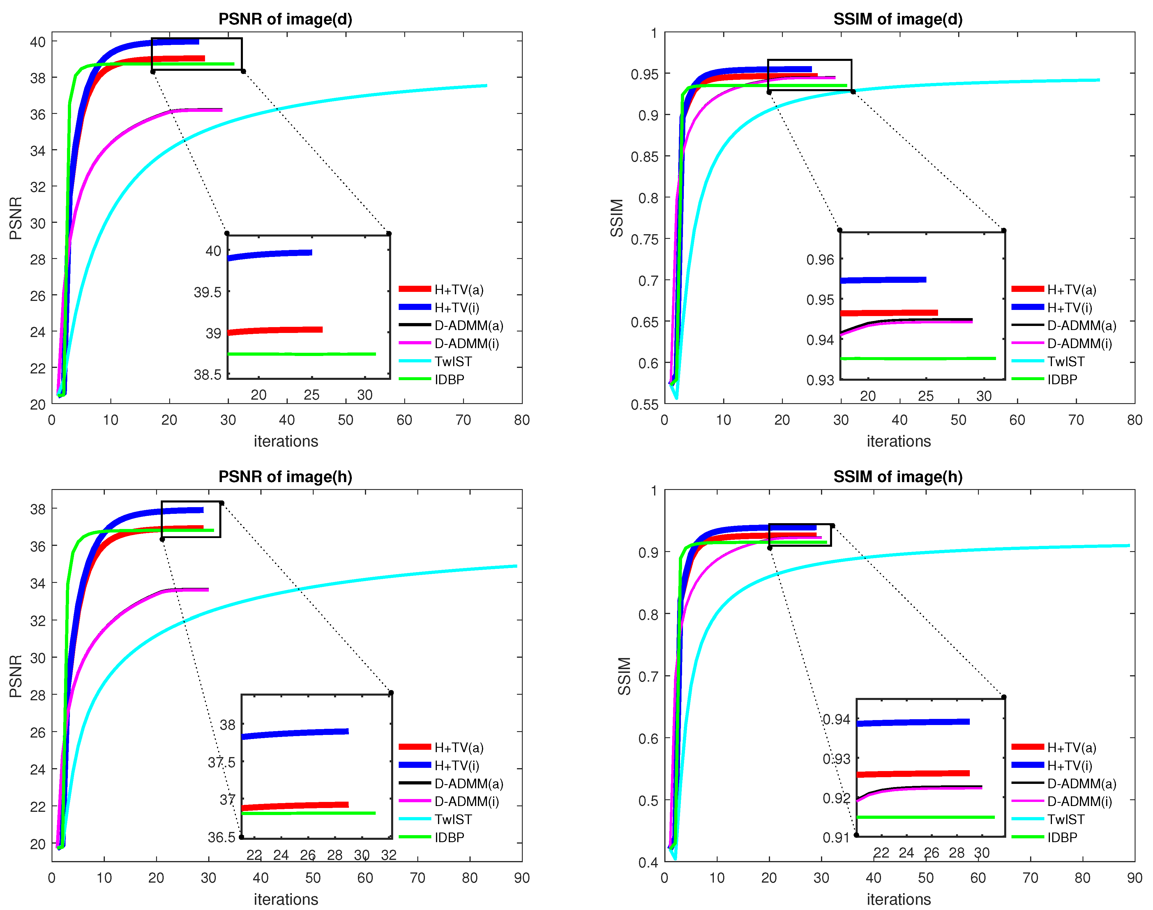
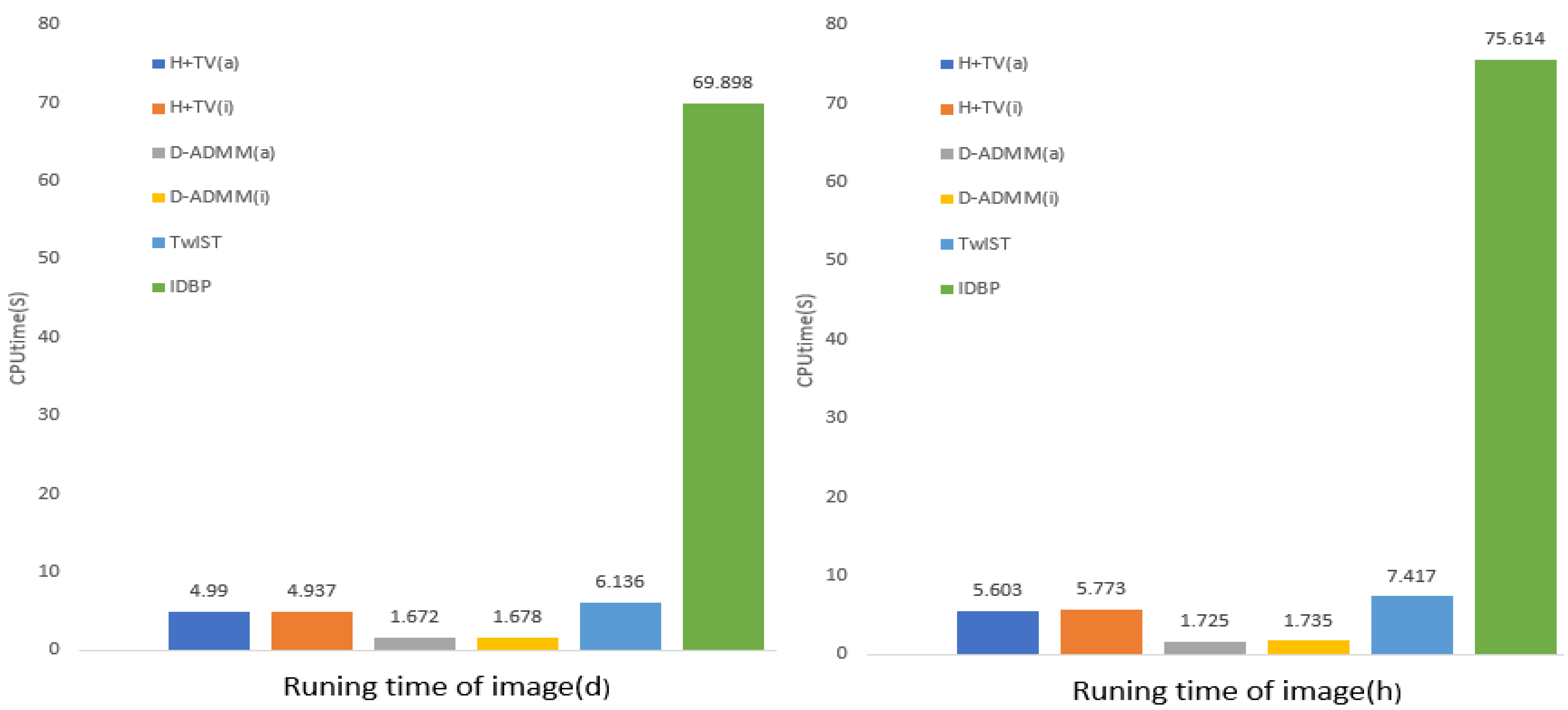
  • Numerical experiments compared with the competitive methods show that the proposed method can obtain better restoration results and computational efficiency.
The rest of this paper is organized as follows. In Section 2, we briefly review some related works on the split Bregman method. In Section 3, the improved model and its minimizing process are presented. The numerical experiments to verify the effect and efficiency of the proposed model are presented in Section 4. Finally, we conclude the paper in Section 5.

2. Related Work

The purpose of splitting Bregman [20] is to transform the difficult 2 T V problem into a sequence of easy-solving subproblems and Bregman updates. By denoting x T V = D x 1 , problem (3) can be written as:
min x 1 2 y H x 2 2 + λ D x 1 ,
where D = D h T , D v T T is the discrete gradient operator, D h x = x i , l + 1 x i , l , D v x = x i + 1 , l x i , l . Let d = d h T , d v T T , with  d h = D h x , d v = D v x . The anisotropic TV [31,32] can then be formulated as d 1 = d h + d v , while the isotropic TV [31,32] can be denoted as d 1 = d h 2 + d v 2 . Thus, the unconstrained optimization problem (4) can be transformed into an equivalent constrained optimization problem (5):
min x 1 2 y H x 2 2 + λ d 1 s . t . d = D x .
Similar to Bregman iterative denoising, (5) is firstly converted into the following two-phase algorithm:
x k + 1 , d k + 1 = a r g min x , d 1 2 y H x 2 2 + λ d 1 + δ 2 d D x b k 2 2 , b k + 1 = b k + D x k + 1 d k + 1 ,
where b k is generated by Bregman distance.
Furthermore, by the splitting criteria, (6) can be broken into three easy steps, resulting in the following simpler subproblems:
S t e p 1 : x k + 1 = a r g min x y H x 2 2 + δ 2 d k D x b k 2 2 , S t e p 2 : d k + 1 = a r g min d λ d 1 + δ 2 d D x k + 1 b k 2 2 , S t e p 3 : b k + 1 = b k + D x k + 1 d k + 1 .
The first step is a perfect differentiable optimization problem that can be directly solved by many mathematical tools. The second step is a typical image denoising problem that can be solved by the shrinkage operator, while the last step involves the addition and subtraction of matrixes.

3. The Proposed Algorithm

In this work, we focus on an improved image restoration method (3) by combining a typically equivalent fidelity term with TV regularization. This equivalent fidelity sought is a pseudoinverse of the full row rank matrix and is defined as a seminorm instead of a real norm [4]. When combined with (3), we obtain the following equivalently constrained optimization form:
min x 1 2 σ e 2 H + y x H T H 2 + λ x T V ,
where H + H T ( H H T ) 1 is the pseudoinverse of H, u H T H 2 u T H T H u is a seminorm and Gaussian random variables n i N 0 , σ e 2 .
By setting y + = H + y , (7) becomes:
min x , y + 1 2 σ e 2 y + x H T H 2 + λ x T V s . t . y + = H + y .
Furthermore, to address the issue caused by the null space of H, with left multiplication of H in y + = H + y , a new constraint H y + = y is firstly obtained to replace the equality constraint in (8). For the current seminorm fidelity term, components of H still exists. In order to estimate the complication caused by null space of H and σ e = 0 , the Euclidean norm 1 σ e + ϵ 2 y + x 2 2 is employed to replace the seminorm in (8) [6]. On the one hand, ϵ > 0 can eliminate the adverse effect of σ e = 0 . On the other hand, by this replacement, the subproblem of solving y + becomes a standard equality constrained quadratic programming problem which can be easily solved by the projection method, while the seeking of x develops into a denoising problem which can be solved conveniently in the split framework. Hence,
min x , y + 1 2 σ e + ϵ 2 y + x 2 2 + λ x T V s . t . H y + = y .
Consequently, (9) is an improved TV-based image restoration method equivalent to (3). Using such transformations, we can ignore the impact of the null space of H in (3) and take advantage of the capacities in noise suppressing and detail preserving of TV norm. Particularly, (9) is a constrained optimization problem with specific regularization and can be conveniently evaluated by adopting a series of mergers and splits, resulting in a sequence of easy-solving subproblems and some matrix updates. In contrast, [4] employed a BM3D denoiser for uncertain φ ( x ) with more time expansion and over smoothing.
By the definition of TV in anisotropic TV and isotropic TV, for solving the anisotropic TV-based image restoration problem, (9) can be formulated as:
min x , y + 1 2 σ e + ϵ 2 y + x 2 2 + λ D h x + λ D v x s . t . H y + = y .
By introducing auxiliary variables d h = D h x and d v = D v x , (10) can be equivalently formulated as:
min x , y + 1 2 σ e + ϵ 2 y + x 2 2 + λ d h + λ d v s . t . H y + = y , d h = D h x , d v = D v x ,
under the split Bregman transition framework, we obtain:
min x , y + , d h , d v 1 2 σ e + ϵ 2 y + x 2 2 + λ d h + λ d v + δ 2 d h D h x b h k 2 2 + δ 2 d v D v x b v k 2 2 s . t . H y + = y ,
where b h k and b v k are generated by Bregman distance.
Thus, we can iteratively estimate an optimal solution of (12) by separating it into four simple sub-problems and updates as follows:
x k + 1 = a r g min x 1 2 σ e + ϵ 2 y + k x 2 2 + δ 2 d h k D h x b h k 2 2 + δ 2 d v k D v x b v k 2 2 ,
d h k + 1 = a r g min d h λ d h + δ 2 d h D h x k + 1 b h k 2 2 ,
d v k + 1 = a r g min d v λ d v + δ 2 d v D v x k + 1 b v k 2 2 ,
y + k + 1 = a r g min y + y + x k + 1 2 2 s . t . H y + = y .
Equation (13) is now a differentiable optimization problem. By setting the gradient of the objective function equal to 0, a system of linear equations is established as follows:
1 σ e + ϵ 2 I n + δ D h T D h + δ D v T D v x = 1 σ e + ϵ 2 y + k + δ D h T d h k b h k + δ D v T d v k b v k .
Obviously, (17) can be directly solved by tools like Fourier transform, Gauss–Seidel, conjugate gradient (CG), etc…. In this study, we employ Gauss–Seidel to complete the iterative process because the main computational cost per iteration is a small number of matrix-scalar multiplications and matrix additions, resulting in satisfied efficiency.
d h k + 1 , d v k + 1 ,which follows regular 2 1 denoising models, can be efficiently estimated using the Shrinkage operators.
d h k + 1 = s h r i n k ( D h x k + 1 + b h k , λ δ ) ,
d v k + 1 = s h r i n k ( D v x k + 1 + b v k , λ δ ) .
Moreover, a closed-form solution of (16) can be efficiently implemented by projecting x k + 1 onto the affine subspace H R n = y as in (20):
y + k + 1 = H + y + ( I n H + H ) x k + 1 .
Finally, b h k and b v k are updated as in (21) and (22), respectively. When some optimal values of b h k and b v k are found, we have b h k + 1 = b h k and b v k + 1 = b v k , hence d h k + 1 = D h x k + 1 , d v k + 1 = D v x k + 1 are explicitly established.
b h k + 1 = b h k + ( D h x k + 1 d h k + 1 ) ,
b v k + 1 = b v k + ( D v x k + 1 d v k + 1 ) .
The variable y + k + 1 is expected to be closer to the true signal x than the raw observations y. Thus, our algorithm alternates between estimating the signal and using this estimation to obtain improved measurements (that comply with the original observations y).
The proposed anisotropic TV algorithm is presented in Algorithm 1.
Algorithm 1 Anisotropic H + T V     H + T V a
1:
Initialize y + 0 , x 0 , d v 0 , d h 0 , b v 0 , b h 0 , k = 0 ;
2:
repeat
3:
     x k + 1 = G x k ;          % Gauss–Seidel iteraction
4:
     d h k + 1 = s h r i n k ( D h x k + 1 + b h k , λ δ ) ;
5:
     d v k + 1 = s h r i n k ( D v x k + 1 + b v k , λ δ ) ;
6:
     b h k + 1 = b h k + ( D h x k + 1 d h k + 1 ) ;
7:
     b v k + 1 = b v k + ( D v x k + 1 d v k + 1 ) ;
8:
     y + k + 1 = H + y + ( I n H + H ) x k + 1 ;
9:
     k = k + 1
10:
until x k x k + 1 2 2 x k 2 2 < t       % t is a threshold of stop critertion
For isotropic TV, (12) can be formulated as a formula of isotropic TV form:
min x , y + , d h , d v 1 2 σ e + ϵ 2 y + x 2 2 + λ d h 2 + d v 2 + δ 2 d h D h x b h k 2 2 + δ 2 d v D v x b v k 2 2 s . t . H y + = y .
It can also separate into four simple sub-problems and updates. For x, y + , b h , and b v , they are solved and updated in the same maner as in anisotropic TV, and we now have to solve d h and d v using the generalized shrinkage formula.
d h k + 1 = max s k λ δ , 0 D h x k + b h k s k ,
d v k + 1 = max s k λ δ , 0 D v x k + b v k s k ,
where
s k = D h x k + b h k 2 + D v x k + b v k 2 .
The proposed isotropic TV algorithm is presented in Algorithm 2
Algorithm 2 Isotropic
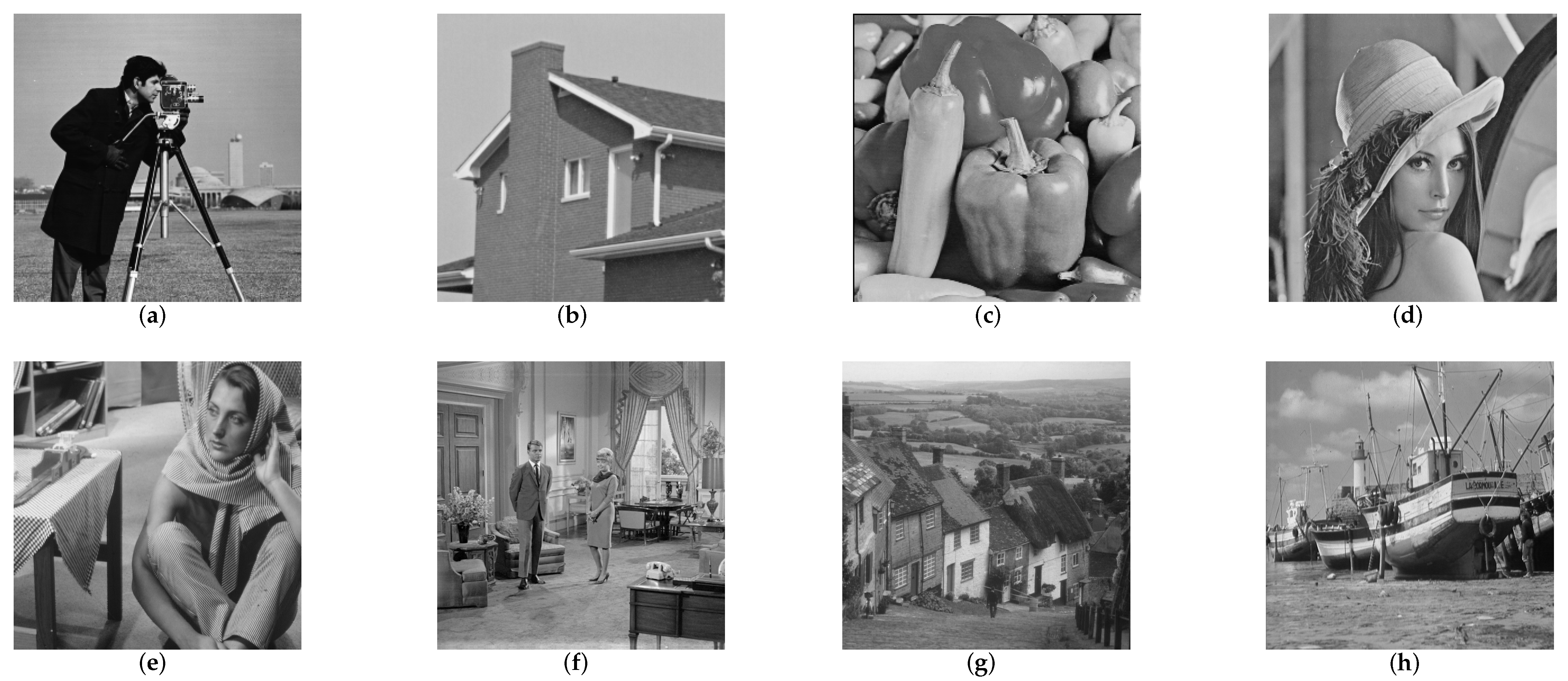
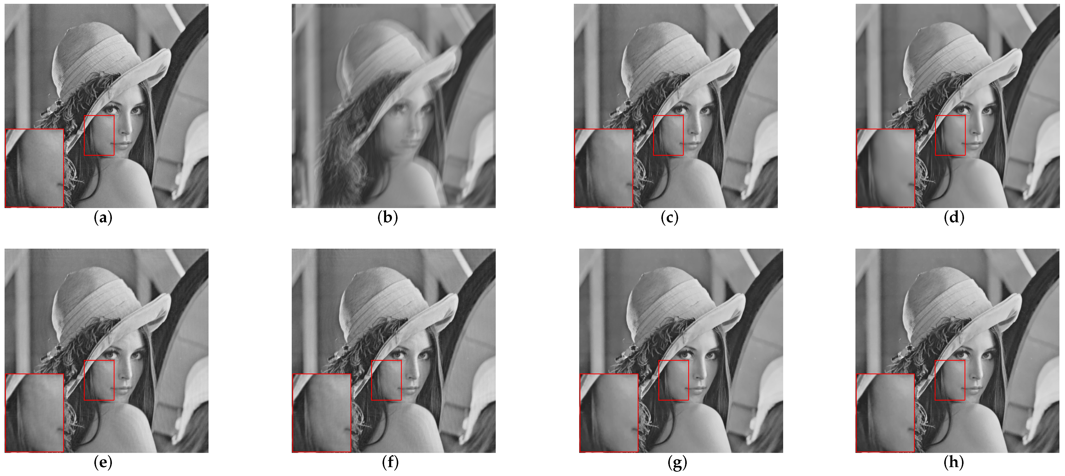
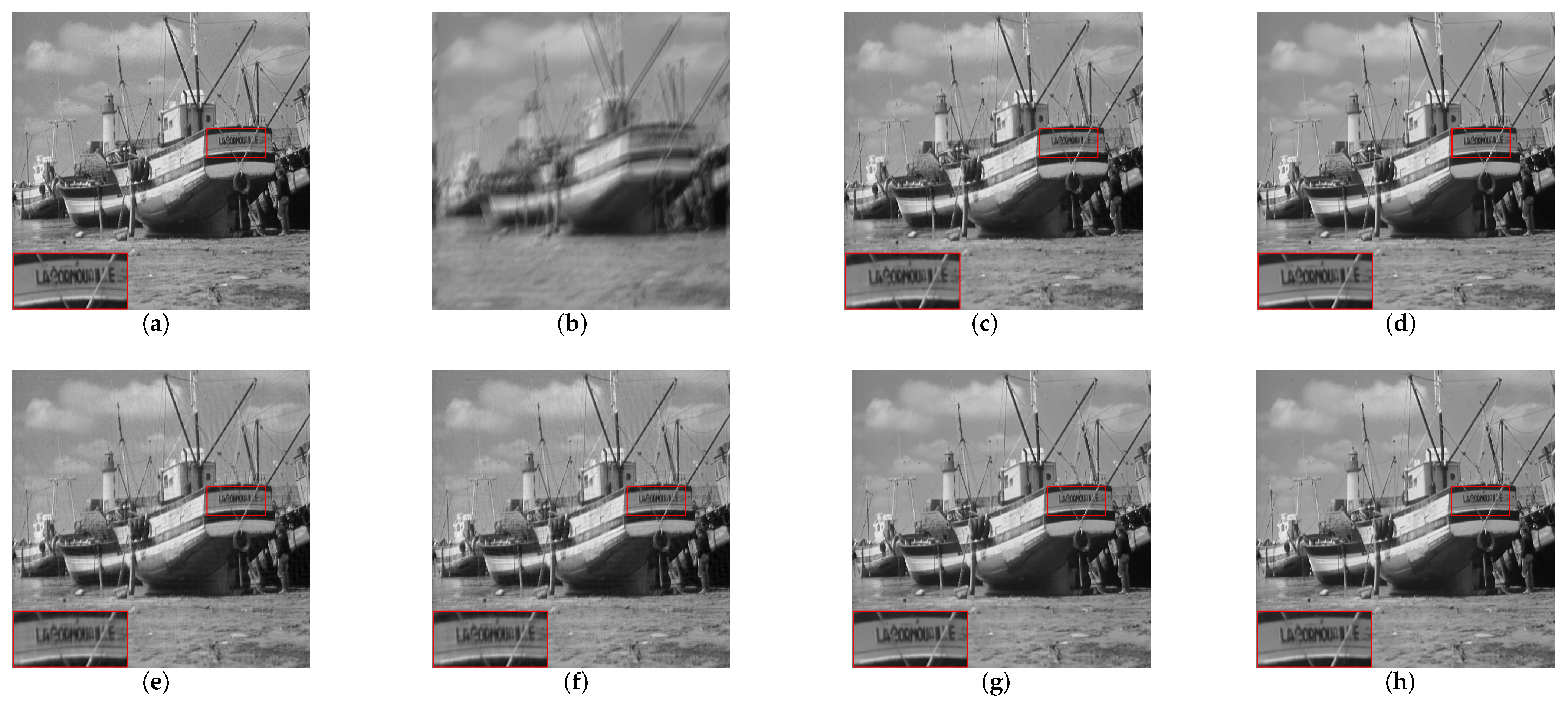
 H + T V     H + T V i
1:
Initialize y + 0 , x 0 , d v 0 , d h 0 , b v 0 , b h 0 , k = 0 ;
2:
repeat
3:
     x k + 1 = G x k ;          % Gauss–Seidel iteraction
4:
     d h k + 1 = max s k λ δ , 0 D h x k + b h k s k ,
5:
     d v k + 1 = max s k λ δ , 0 D v x k + b v k s k ,
6:
     b h k + 1 = b h k + ( D h x k + 1 d h k + 1 ) ;
7:
     b v k + 1 = b v k + ( D v x k + 1 d v k + 1 ) ;
8:
     y + k + 1 = H + y + ( I n H + H ) x k + 1 ;
9:
     k = k + 1
10:
until x k x k + 1 2 2 x k 2 2 < t          % t is a threshold of stop critertion

4. Experiments

This section examines the effect of the proposed method using the eight 256 × 256 test images shown in Figure 1. The H + T V algorithm was implemented in MATLAB 2016a and generated on a 2.90 GHz Core (TM) i5-10400F PC with 16 GB of memory.
In our experiments, camera shake kernels used in [2,33] and Gaussian white noise are chosen to generate the degraded images. State-of-the-art image restoration methods, such as D-ADMM [5] (including anisotropic D-ADMM and isotropic D-ADMM, i.e., D-ADMM (a) and D-ADMM (i)), IDBP [6], and TwIST [13] are listed in comparative experiments. For regularization parameters, we set λ = 2 and the stop criterion threshold t = 1 × 10 4 . Peak to Peak Signal to Noise Ratio (PSNR) and Structure Similarity Index Measure (SSIM) are employed to evaluate the quality of image restoration.
In the experiments, test images are blurred by the kernel =   k 4 [33]. Gaussian white noise with zero mean value and the standard deviation of 1 × 10 3 is added to the blurred images to generate the degraded images. Table 1 and Table 2 list the PSNR and SSIM to evaluate the restoration effectiveness of the algorithms. For all test images, the anisotropic H + T V and isotropic H + T V can consistently achieve comparable or better restoration quality than others, especially in terms of SSIM values. Although IDBP achieves better PSNR for two of the test images, its SSIM is lower than the proposed methods, indicating the better detail and structure preserving capability of our algorithms.
In order to achieve a distinct visual effect, Figure 2 and Figure 3 show the restoration results with the proposed and competed comparison methods in Figure 1d,h. Figure 2g–h and Figure 3g–h show that anisotropic H + T V and isotropic H + T V are more effective for denoising and small details preserving like edges and lines, especially in the enlarged area.
A more critical indicator for evaluating the efficiency of the different algorithms was obtained by listing the iteration and running time of each competing algorithm. To obtain a more distinct contrast effect, taking images Figure 1d,h as examples, we plot the evolution curves of PSNR and SSIM, along with the number of iterations in Figure 4. To get a better contrast, we zoom in the final values of PSNR and SSIM in Figure 4. In addition, the time required to reach the stop criterion is plotted in Figure 5, and the proposed method is several times faster than IDBP. Although D-ADMM is faster than our method, both the image restored indicator of PSNR and SSIM are lower. Besides, our approach performs better than TwIST, both in terms of running CPU time and quality.

5. Conclusions

In this work, an improved TV-based objective function for image restoration is proposed. By constructing a pseudoinverse matrix, an equivalent seminorm fidelity term-based TV optimization problem is established. An efficient splitting minimization scheme, including anisotropic H + T V and isotropic H + T V are employed for solving the improved problem. Compared with the state-of-the-art D-ADMM, IDBP, and TwIST methods, the experimental results demonstrated that the proposed methods could obtain satisfactory restoration results with fewer iterations. The proposed algorithms could also be extended to other image restoration applications, e.g., image inpainting, compressed sensing, and image construction. The proposed method was mainly about image restoration from degraded ones of blur and additive Gaussian white noise, and is limited for mixed noise.

Author Contributions

G.M. and Z.Y. developed the idea that resulted in this paper and were responsible for the experimental collation; Z.L. contributed to the design of experiments; Z.Z. contributed to manuscript writing; All authors have read and agreed to the published version of the manuscript.

Funding

This project was supported by the National Natural Science Foundation of China (grant Nos. 61803110, 62173102), the Natural Science Foundation of Guangdong Province, China (grant No. 2018A030310065), and the Science and Technology Planning Project of Guangzhou, China (grant No. 202102020876).

Institutional Review Board Statement

Not applicable.

Informed Consent Statement

Not applicable.

Data Availability Statement

Enquiries regarding experimental data should be made by contacting the first author.

Conflicts of Interest

The authors declare no conflict of interest.

References

  1. Banham, M.R.; Katsaggelos, A.K. Katsaggelos Digital Image Restoration. IEEE Signal Process. Mag. 1997, 14, 24–41. [Google Scholar] [CrossRef]
  2. Tikhonov, A.N.; Arsenin, V.Y. Solutions of Ill-Posed Problems. Math. Comput. 1978, 32, 1320–1322. [Google Scholar]
  3. Chen, S.S. Atomic Decomposition by Basis Pursuit. SIAM Rev. 2001, 43, 129–159. [Google Scholar] [CrossRef] [Green Version]
  4. Rudin, L.I.; Osher, S.; Fatemi, E. Nonlinear Total Variation Based Noise Removal Algorithms. Phys. D Nonlinear Phenom. 1992, 60, 259–268. [Google Scholar] [CrossRef]
  5. Ren, D.; Zhang, H.; Zhang, D.; Zuo, W. Fast Total-Variation Based Image Restoration Based on Derivative Alternated Direction Optimization Methods. Neurocomputing 2015, 170, 201–212. [Google Scholar] [CrossRef]
  6. Tirer, T.; Giryes, R. Image Restoration by Iterative Denoising and Backward Projections. IEEE Trans. Image Process. 2018, 28, 1220–1234. [Google Scholar] [CrossRef]
  7. Daubechies, I.; Defrise, M. An Iterative Thresholding Algorithm for Linear Inverse Problems with a Sparsity Constraint. Commun. Pure Appl. Math. A J. Issued Courant Inst. Math. Sci. 2004, 57, 1413–1457. [Google Scholar] [CrossRef] [Green Version]
  8. Elad, M. Why Simple Shrinkage Is Still Relevant for Redundant Representations? IEEE Trans. Inform. 2006, 52, 5559–5569. [Google Scholar] [CrossRef]
  9. Elad, M.; Matalon, B.; Zibulevsky, M. Image Denoising with Shrinkage and Redundant Representations. In Proceedings of the 2006 IEEE Computer Society Conference on Computer Vision and Pattern Recognition (CVPR), New York, NY, USA, 22 June 2006; pp. 1924–1931. [Google Scholar]
  10. Starck, J.L.; Donoho, D.L.; Candès, E.J. Astronomical Image Representation by the Curvelet Transform. A&A 2003, 398, 785–800. [Google Scholar]
  11. Starck, J.L.; Nguyen, M.K.; Murtagh, F. Wavelets and Curvelets for Image Deconvolution: A Combined Approach. Signal Process. 2003, 83, 2279–2283. [Google Scholar] [CrossRef]
  12. Figueiredo, M.A.T.; Nowak, R.D.; Wright, S.J. Gradient Projection for Sparse Reconstruction: Application to Compressed Sensing and Other Inverse Problems. IEEE J. Sel. Top. Signal Process. 2007, 1, 586–597. [Google Scholar] [CrossRef] [Green Version]
  13. Bioucas-Dias, J.M.; Figueiredo, M.A.T. A New TwIST: Two-Step Iterative Shrinkage/Thresholding Algorithms for Image Restoration. IEEE Trans. Image Process. 2007, 16, 2992–3004. [Google Scholar] [CrossRef] [PubMed] [Green Version]
  14. Beck, A.; Teboulle, M. A Fast Iterative Shrinkage-Thresholding Algorithm for Linear Inverse Problems. SIAM J. Imaging Sci. 2009, 2, 183–202. [Google Scholar] [CrossRef] [Green Version]
  15. Ma, G.; Hu, Y.; Gao, H. An Accelerated Momentum Based Gradient Projection Method for Image Deblurring. In Proceedings of the 2015 IEEE International Conference on Signal Processing, Communications and Computing (ICSPCC), Ningbo, China, 19–22 September 2015; pp. 1–4. [Google Scholar]
  16. Afonso, M.V.; Bioucas-Dias, J.M.; Figueiredo, M.A.T. Fast Image Recovery Using Variable Splitting and Constrained Optimization. IEEE Trans. Image Process. 2010, 19, 2345–2356. [Google Scholar] [CrossRef] [Green Version]
  17. Afonso, M.V.; Bioucas-Dias, J.M.; Figueiredo, M.A.T. An Augmented Lagrangian Approach to the Constrained Optimization Formulation of Imaging Inverse Problems. IEEE Trans. Image Process. 2011, 20, 681–695. [Google Scholar] [CrossRef] [PubMed] [Green Version]
  18. Osher, S.; Burger, M.; Goldfarb, D.; Xu, J.; Yin, W. An Iterative Regularization Method for Total Variation-Based Image Restoration. Multiscale Model. Simul. 2005, 4, 460–498. [Google Scholar] [CrossRef]
  19. Yin, W.; Osher, S.; Goldfarb, D.; Darbon, J. Bregman Iterative Algorithms for l1-Minimization with Applications to Compressed Sensing. SIAM J. Imaging Sci. 2008, 1, 143–168. [Google Scholar] [CrossRef] [Green Version]
  20. Goldstein, T.; Osher, S. The Split Bregman Method for L1-Regularized Problems. SIAM J. Imaging Sci. 2009, 2, 323–343. [Google Scholar] [CrossRef]
  21. Buades, A.; Coll, B.; Morel, J.-M. A Non-Local Algorithm for Image Denoising. In Proceedings of the 2005 IEEE Computer Society Conference on Computer Vision and Pattern Recognition (CVPR), San Diego, CA, USA, 20–26 June 2005; pp. 60–65. [Google Scholar]
  22. Dabov, K.; Foi, A.; Katkovnik, V.; Egiazarian, K. Image Denoising by Sparse 3-D Transform-Domain Collaborative Filtering. IEEE Trans. Image Process. 2007, 16, 2080–2095. [Google Scholar] [CrossRef]
  23. Tomasi, C.; Manduchi, R. Bilateral Filtering for Gray and Color Images. In Proceedings of the Sixth International Conference on Computer Vision (ICCV), Narosa Publishing House, Bombay, India, 4–7 January 1998; pp. 839–846. [Google Scholar]
  24. Khan, A.; Jin, W.; Haider, A.; Rahman, M.; Wang, D. Adversarial Gaussian Denoiser for Multiple-Level Image Denoising. Sensors 2021, 261, 2998. [Google Scholar] [CrossRef]
  25. Yang, C.; Huang, D.; He, W.; Cheng, L. Neural Control of Robot Manipulators With Trajectory Tracking Constraints and Input Saturation. IEEE Trans. Neural Netw. Learn. Syst. 2021, 32, 4231–4242. [Google Scholar] [CrossRef] [PubMed]
  26. Yang, C.; Chen, C.; He, W.; Cui, R.; Li, Z. Robot Learning System Based on Adaptive Neural Control and Dynamic Movement Primitives. IEEE Trans. Neural Netw. Learn. Syst. 2019, 30, 777–787. [Google Scholar] [CrossRef]
  27. Burger, H.C.; Schuler, C.J.; Harmeling, S. Image Denoising: Can Plain Neural Networks Compete with BM3D? In Proceedings of the 2012 IEEE Conference on Computer Vision and Pattern Recognition(CVPR), Providence, RI, USA, 16–21 June 2012; pp. 2392–2399. [Google Scholar]
  28. Wang, Y.; Song, X.; Gong, G.; Li, N. A Multi-Scale Feature Extraction-Based Normalized Attention Neural Network for Image Denoising. Electronics 2021, 10, 319. [Google Scholar] [CrossRef]
  29. Shao, L.; Zhang, E.; Li, M. An Efficient Convolutional Neural Network Model Combined with Attention Mechanism for Inverse Halftoning. Electronics 2021, 10, 1574. [Google Scholar] [CrossRef]
  30. Cho, S.I.; Park, J.H.; Kang, S.-J. A Generative Adversarial Network-Based Image Denoiser Controlling Heterogeneous Losses. Sensors 2021, 21, 1191. [Google Scholar] [CrossRef] [PubMed]
  31. Beck, A.; Teboulle, M. Fast Gradient-Based Algorithms for Constrained Total Variation Image Denoising and Deblurring Problems. IEEE Trans. Image Process. 2009, 18, 2419–2434. [Google Scholar] [CrossRef] [PubMed] [Green Version]
  32. Zuo, W.; Lin, Z. A Generalized Accelerated Proximal Gradient Approach for Total-Variation-Based Image Restoration. IEEE Trans. Image Process. 2011, 20, 2748–2759. [Google Scholar] [CrossRef]
  33. Levin, A.; Weiss, Y.; Durand, F.; Freeman, W.T. Understanding and evaluating blind deconvolution algorithms. In Proceedings of the 2009 IEEE Conference Computer Vision and Pattern Recognition (CVPR), Miami, FL, USA, 20–25 June 2009; pp. 1964–1971. [Google Scholar]
Figure 1. Eight test images used in our experiments. (a) Cameraman. (b) House. (c) Peppers. (d) Lena. (e) Barbara. (f) Couple. (g) Hill. (h) Boat.
Electronics 11 00258 g001
Figure 2. Recovered results results of image (d) obtained using different algorithms. (a) Original. (b) Degraded. (c) TwIST. (d) IDBP. (e) D-ADMM (a). (f) D-ADMM (i). (g) H + T V (a). (h) H + T V (i).
Electronics 11 00258 g002
Figure 3. Recovered results results of image (f) obtained using different algorithms. (a) Original. (b) Degraded. (c) TwIST. (d) IDBP. (e) D-ADMM (a). (f) D-ADMM (i). (g) H + T V (a). (h) H + T V (i).
Electronics 11 00258 g003
Figure 4. Iteration-varying of PSNR and SSIM.
Electronics 11 00258 g004
Figure 5. Running time comparison of different algorithms.
Electronics 11 00258 g005
Table 1. Comparison of PSNR values of each method in eight plots.
Method H + TV  (a) H + TV  (i)D-ADMM (a)D-ADMM (i)TwISTIDBP
Cameraman37.8739.0130.7530.7035.3339.10
House38.8039.7134.7634.6537.3039.56
Peppers38.9839.9032.5632.4836.5038.42
Lena39.0339.9736.2136.1837.5438.74
Barbara35.6737.0329.5629.5631.3639.12
Boat36.9237.9033.6333.6034.8936.81
Hill36.9037.9634.6634.6434.7536.49
Couple37.3238.2534.5333.4734.3137.49
Table 2. Comparison of SSIM values of each method in eight plots.
Method H + TV  (a) H + TV  (i)D-ADMM (a)D-ADMM (i)TwISTIDBP
Cameraman0.9570.9640.8960.8930.9420.956
House0.9340.9460.9160.9130.9230.946
Peppers0.9630.9680.9130.9110.9520.951
Lena0.9460.9540.9440.9440.9440.935
Barbara0.9510.9610.8930.8920.9150.960
Boat0.9260.9390.9220.9220.9090.914
Hill0.9330.9470.9210.9200.9080.922
Couple0.9440.9540.9290.9280.9210.937
Publisher’s Note: MDPI stays neutral with regard to jurisdictional claims in published maps and institutional affiliations.

