1. Introduction
Embedded systems can be found in nearly every modern electronic device ranging from home appliances, medical devices, mobile devices, industrial equipment to office machines, and automobiles. As a result, recent trends are now turning towards coupling these ubiquitous embedded devices with machine-learning models to provide built-in device intelligence. Most of this work has centered around embedded deep learning, which is a specific category of machine learning that focuses on Deep Neural Networks (DNN) architectures.
DNNs are widely used in a number of embedded application areas including computer vision [
1,
2,
3,
4], speech recognition [
5,
6], language processing [
7,
8], robotics, and healthcare [
9]. However, due to the large volume of data required to create accurate models in many cases, and the significant amount of computing resources needed to train the models, training is usually performed in high-performance computing (HPC) environments. However, once the model has been trained, initial research has shown that it can be effectively executed on embedded processors or other resource constrained devices [
10,
11,
12,
13,
14]. The running of machine learning models on these embedded devices is commonly referred to as embedded machine learning (EML) [
15].
The implications of this approach are that through the effective utilization of EML there is the potential for unlocking the processing of data within the billions of embedded devices which are already available in a number of environmental settings (e.g., industrial factories, smart buildings, residential complexes …). This indicates that the processing of data that is already being produced by these devices can now be exploited, most of which is currently being under-utilized.
In addition to the potential for improved utilization of all these embedded devices, there are other benefits to be gained from performing inference on the embedded devices rather than using the conventional HPC-based approach.
Lower Latency: EML is more efficient than traditional cloud-based ML where timeliness is important. The reason is with EML there would no longer be the requirement to transfer a large amount of network data to the cloud. As a result, EML could be an ideal solution to support various real-time applications such as actuation which require lower latencies in order for the control algorithms to perform correctly.
Power Consumption: Many embedded system processors, such as microcontrollers, are much more power-efficient than their HPC-based counterparts. For example, a single Nvidia V100 GPU can consume approximately 300 watts of power per hour.
Network Bandwidth: Running the machine learning models directly on the embedded devices allows for the extraction features and analysis of data directly at the source of the data. This eliminates the need for transferring large amounts of raw data to the network edge or to cloud-based servers, which reduces network bandwidth.
Privacy/Security: Since EML devices would not require an Internet connection there would be no need to transfer and store the data in the cloud. This reduces the risk of data breaches and security leaks providing a higher degree of protection
It is obvious that the broader impact for EML is significant and with over 38.2 billion embedded processors projected to be sold in 2023, the potential benefit could impact practically every major industry. However, while some progress has been made in EML there are still a number of challenges that require consideration in order for this technology to reach its full potential. For one, it will be necessary to deploy the inference part of the machine learning algorithm onto an embedded platform. This deployment has its own unique set of challenges and requirements. For instance, most ML frameworks are not optimized for embedded devices because the models are too large and computationally expensive for resource constrained devices. Consequently, there has been a significant amount of research that has focused on compressing the DNN models to fit into a specific embedded platform and then subsequently mapped onto the appropriate processing element. However, managing the diverse interfaces between the available hardware resources—which are often numerous and heterogeneous in nature—becomes increasingly difficult when performed offline or during design time. The reason is at runtime the amount of computing resources available to a DNN can vary considerably due to the combination of diverse and dynamic workloads concurrently running on the embedded platform.
Some of the challenges listed above suggest that in order to provide a more broad based solution to EML a dynamic runtime approach is needed. Because different hardware platforms have varying computing resources and specific DNNs have different performance requirements various methods will be needed to adapt to the different DNN models for specific hardware. Authors in [
16] proposed that this hardware diversity can be solved at design time by right-sizing the DNN for the specific target platform. For example, the same DNN could run on one platform uncompressed while running a compressed version on a different hardware platform. While design-time approaches can be used to fit the model to the hardware at runtime the available computing resources could vary considerably based on the number of applications running. As mentioned by Xun, Lei et al. [
16,
17,
18,
19] current approaches for EML mainly focus on hardware or algorithm optimizations. Other research [
20,
21,
22,
23] has focused on optimization opportunities in either applications or hardware devices. However, it is important to explore other opportunities of the system as a whole and not just the application or devices based upon the diversity of computation on an embedded platform.
While various runtime management approaches exist in the literature for optimizing system behavior, such as dynamic voltage and frequency scaling (DVFS), dynamic task mapping or thread migration, they are typically implemented for a specific platform or specific applications. Therefore, in order to explore these opportunities, we present the architecture for a new dynamic runtime resource allocation framework (QoS-EML) that can be applied across a range of embedded platforms and machine learning applications. Where the main contribution of this work is to provide a resource allocation scheme that utilizes feedback mechanisms to monitor compute capacity and control quality-of-service (QoS) levels to guarantee a certain level of system performance even when the task workload or resource availability is not known a priori.
The details of QoS-EML are defined in this paper and organized as follows:
Section 2 provides an overview of the resource allocation framework for EML.
Section 3 provides some implementation details while
Section 4 discusses the results of QoS-EML with simulated workloads.
Section 5 discusses provides the details of implementing the framework on a Raspberry Pi 4 as well as some application results running Tensorflow Lite.
Section 6 discusses some related work where results are discussed and compared and
Section 7 provides a summary of the work along with recommendations for future work.
2. Dynamic QoS-Based Resource Allocation for EML
Many EML applications could have varying or unpredictable execution rates. For example, the runtime of inference execution could vary considerably depending upon the compression level of the DNN model. Additionally, dynamic voltage and frequency scaling (DVFS) techniques which are used to provide a balance between energy consumption and performance that are widely used in modern architecture can also contribute to the varying execution rates.
A primary limitation to providing a more dynamic approach is that most general-purpose operating systems (e.g., Linux) provide timesharing scheduling algorithms where the controlling executing rate is not supported. These time-sharing algorithms are best-effort where tasks can easily overload the processor by simply creating enough processes. Therefore, a service level control mechanism is important to be able to isolate the execution rate of different applications, which means embedded applications may need to change their QoS requirements during runtime. For instance, one model could have higher accuracy requirements which may take longer to execute while another model may be able to sufficiently sacrifice accuracy for performance. In order to address some of these limitations, we provide a more dynamic QoS-based resource allocation approach.
With our approach resource allocation includes both task mapping and task scheduling for the embedded platform. Where the role of the task mapper is to assign tasks to be executed on a particular processing unit while the task scheduler runs the scheduling algorithms, which in our case is a non-preemptive earliest deadline first (C-EDF) scheduler. The following sections are set aside to provide more details about the implementation of a QoS-based resource allocation approach that uses feedback-based heuristics to guarantee satisfactory performance for resource constrained devices.
Feedback Based Control Heuristics
One of the primary motivations for employing a feedback based approach is that traditional compute platforms are “open loop” which means once resources are scheduled they are unable to be adjusted to accommodate dynamic changes in the system. While open-loop scheduling algorithms have been proven to perform well in dynamic systems where workloads are well-defined, they typically perform do not perform as well in unpredictable dynamic systems, such as robotic or machine learning applications, where workloads and compute times are highly unpredictable.
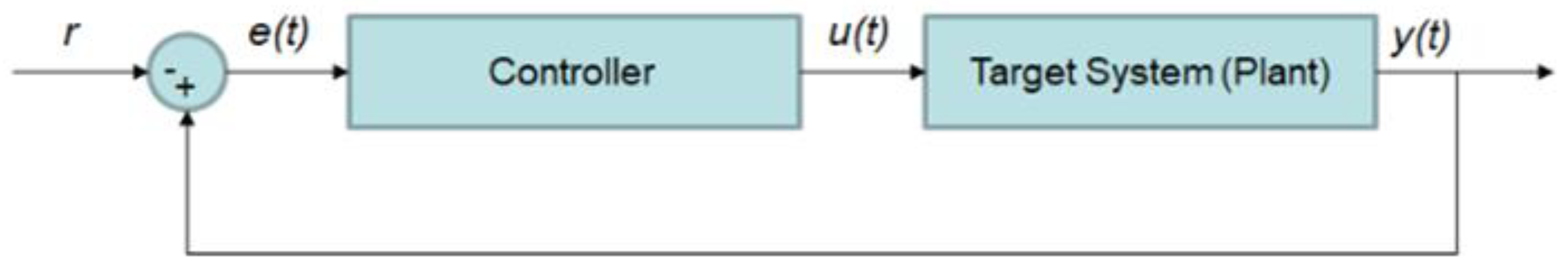
A better solution to the traditional open-loop approach is to periodically monitor the environment and then provide feedback to the system to provide satisfactory performance. This type of feedback would then be able to deal with dynamic systems that are both resource constrained and with unpredictable workloads. Furthermore, by applying these feedback mechanisms (see
Figure 1) the current resource capacity can be monitored so that specific QoS levels could be supported which can guarantee a certain level of performance (e.g., overall system utilization, power consumption or deadline miss ratio).
A typical feedback mechanism consists of a controller, the target system to be controlled (plant), monitors and actuators. The controller variable (y (t)) defines the output of the system that is used by the controller to make adjustments. The set point variable (r) represents the desired value for the controlled variable. The error (e (t)) is defined as the difference between the set point and the controlled variable. The variable (u (t)) is the value that is manipulated by the controller to change the value of the controlled variable.
Typically a proportional-integral-derivative (PID) controller is used to provide the necessary control for feedback based scheduling. The basic time-domain form for PID control is defined as:
Determining the values for the proportional , integral , and derivative components of the controller are known as PID controller tuning.
3. Feedback Control Based Resource Allocation Architecture
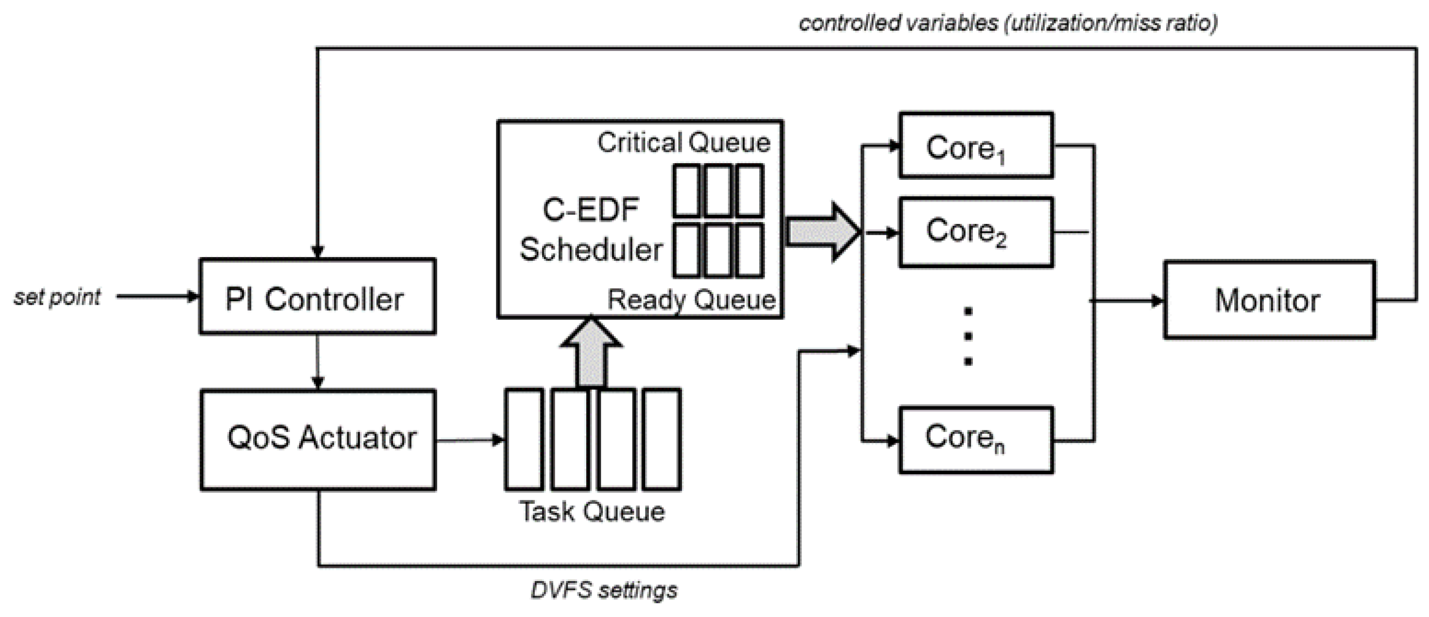
Our feedback control mechanism is based upon the FCS-EDF architecture initially proposed by authors [
20] and consists of several components: a task model, a controller, an admission controller, a QoS actuator and a real-time scheduler. In
Figure 2, an overview of the resource allocation architecture is provided.
3.1. Task Model
The task model assumes that all tasks are soft real-time and independent. Each task is defined as a 5-tuple: . Every task has one or more logical versions where a task with multiple versions may or may not have multiple implementations. Defines the various execution times for each version where define the execution times for different versions. represents the accuracy of different implementations. Dynamic DNNs for instance could have multiple configurations where each version could have different execution times and accuracy levels based upon how the model has been pruned. Different versions of each task are identified as the task’s QoS level where a version with a longer execution time and more precise accuracy is a higher QoS level than another version with a shorter execution time with lower accuracy. The remaining parameters and defines the task start time and relative deadline respectively.
3.2. PI Controller
In order to implement the feedback loop, a few control variables will need to be identified which are the controlled variable, the set point and the manipulated variable. The controlled variable defines the quantity of the output that is measured and controlled. The controlled variable in our case is processor utilization U(t) defined over a time window ((t − 1) W, tW)) where W is the sampling window and t is called the sampling instant. The utilization U(t) at the tth sampling moment represents the amount of time that the processor is busy over the sampling window ((t − 1)W, tW)). The set point represents the desired value for the controlled variable where the difference is between the current value and the set point. In our case, the set point would be a percentage of overall processor utilization defined as U(t). The manipulated variable is the value that can be changed dynamically by the scheduler to affect the controlled variable. In this case, the manipulated variable is the total estimated processor utilization defined as which represents all the tasks in the system, where Ti is a task with a QoS level of Li(t) in the tth sampling window.
This feedback control loop is invoked every sampling instant
t, the controller then calculates the control input defined as
which represents the change in total estimated requested utilization based upon the processor utilization error
. The controller uses a PI (Proportional-Integral) control function to compute the control input defined as:
The controller is tuned based upon the Root Locus Technique [
24] with the following control parameters:
. Algorithm 1 based on the design in [
20] provides the pseudo-code of the controller mechanism.
3.3. QoS Actuator
The QoS actuator modifies the requested utilization in the system by adjusting the QoS levels of the accepted tasks. For example, consider that the QoS level of task
changes from
to
then the requested utilization would change by
, where
and
are the estimated processor requirements of
and
, respectively. Algorithm 2 which is based on [
25] and extended to support DVFS provides the pseudo-code for the QoS Actuator Mechanism. After the requested utilization has been calculated the actuator submits the task to the ready queue. The role of the scheduler is to determine which of the processing cores to execute the task. The decision on which core to use is to measure core utilization and typically the core that is the most idle is selected to run the task. The actuator also performs dynamic voltage and frequency scaling (DVFS) which is a power saving technique that adjusts the power and speed of the processor to optimize resource allocation. The idea is to trade off computation performance for energy savings because there is usually no additional benefits from faster task allocation just as long as it is before the task’s deadline.
| Algorithm 1. PI Controller |
Input: processor utilization set point during sampling period ((t − 1)W, tW)
utilization control parameter
Output: The processor utilization adjustment during sample window
1: U = get processor utilization for sampling period
// PI control function
2:
// increase system load if low utilization by tunable load factor
3: if then
4:
5: end if
// call the QoS Actuator to adjust utilization levels of tasks
5:
// adjust if not fully accommodated for by the QoS Actuator
6: if then
7:
8: end if |
DVFS, which is a common power saving technique, provides the capability to adjust the power and speed settings on various chips and peripheral devices to optimize the allocation of power. Most modern operating systems provide support for DVFS where a limited number of discrete voltage and frequency levels are offered. For example, the Advanced Configuration and Power Interface (ACPI) defines four processor states: operating state (C0), halt state (C1), stop-clock state (C2) and sleep state (C3). The C-states with the higher numbers mean less energy is consumed, while the core is in the operating state (C0) it operates within a range of power performance states identified as P-states. In the P0 state, a core operates at the highest frequency and voltage level while the other P-states provide less performance but require less energy as well. It is also important to note that DVFS is offered on a per-core or per-chip basis, however per-core is not as prevalent so for the intent of this paper we only consider per-chip DVFS.
| Algorithm 2. QoS Actuator |
Input: requested processor utilization change DB(t)
Output: The processor utilization adjustment 〖DB〗^’ based upon task QoS settings
1: 〖DB〗^’= DB(t)
2: if 〖DB〗 ^’< 0 then
3: while 〖DB〗 ^’< 0 and LowQosLevel Task Exist do
4: T_i = SelectLowQoSLevelTask( )
// change task QoS level from current level (j) to new level (k)
5: ChangeQoSTaskLevel (T_i, j, k)
6: 〖DB〗^’= 〖DB〗^’− 〖ET〗_ik+ 〖ET〗_ij
7: end while
8: else
9: while 〖DB〗^’> 0 and HighPrio Task Exist do
10: T_i = SelectHighQoSLevelTask( )
// change task QoS level from current level (j) to new level (k)
11: ChangeTaskQoSLevel (T_i, j, k)
12: 〖DB〗^’= 〖DB〗^’− 〖ET〗_ik+ 〖ET〗_ij
13: end while
14: end if
// Adjust voltage and frequency levels of core(s)
15: +V = CheckVoltageLevels()
16: if 〖DB〗^’> +V then
17: IncreaseVoltFreq(coren)
18: end if
19: if 〖DB〗^’< −V then
20: DecreaseVoltFreq(coren)
21: end if |
DVFS scaling is performed by checking the total estimated processor utilization calculated by the controller and tested against two threshold values +V and −V. If then that indicates that the processing core (s) frequency and voltage should be increased. If then that implies that the cores are under-utilized which indicates that the voltage and frequency should be decreased to conserve energy. It is important to find an optimal threshold value for V, where it should be large enough to limit frequent voltage switching. The common guidelines are that voltage switching should only be performed due to a high value of as well as a relatively large value of the integral component which indicates the error value has been larger for a longer interval.
3.4. Real-Time Scheduler
The primary function of the scheduler is to schedule the tasks in the system. For our architecture, all tasks are assumed to be soft real-time so a certain number of missed deadlines are acceptable but a task executed after its deadline is of no value to the user. Furthermore, tasks are non-cooperating independent tasks and not preempted during their runtime. This is due in part to the fact that EML applications typically utilize other co-processors, such as a GPU, which are considered non-preemptive due to the high overhead associated with context switching.
There are a number of non-preemptive scheduling algorithms, such as first-come-first-serve (FCFS), which are not optimal. For our work, we have chosen the non-preemptive earliest deadline first (EDF) policy known as Clairvoyant EDF [
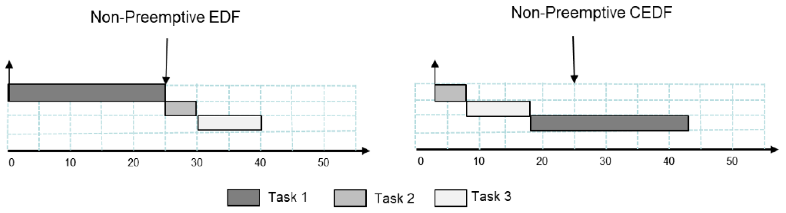
26] which has been shown to be near-optimal for non-preemptive tasks. The basic idea behind C-EDF is sometimes it may not be necessary to dispatch a task that is ready to run but rather delay it—known as inserted idle time. The question is how do you know when to idle a task? There are situations that can be identified where postponing tasks can be beneficial.
For example, if we have two tasks
and
where
but
should
should be postponed? In order to make that determination we need to identify the time interval during which the task must execute to be defined as:
where
and
. Note that the interval is not fixed in that the
value could be increased if a task is postponed, while
could be decreased if another task
cannot start as late. In order to support postponement, CEDF utilizes two queues, the ready queue and a critical queue. The ready queue contains the tasks that have arrived and are ready for execution ordered by their deadlines. The critical queue contains all the tasks according to their
parameters. The following example shown in
Figure 3 is provided to illustrate how the C-EDF algorithm works. (Note: C-EDF only requires the
parameters as the other QoS settings are already determined by the controller and actuator).
Consider the following task set defined as:
= (25, 0, 45),
= (4, 3, 25) and
= (10, 6, 25). The CEDF algorithm would order the tasks in a critical queue based upon
= 20,
= 21,
= 15 so the critical queue would be ordered:
. At time 0 task
the postpone test
is executed and since 0 + 25 > 15
will be postponed to time 6 + 10 = 16. Because
the
parameters will have to be updated for all tasks that satisfy the condition
with regard to
. Therefore,
will be inserted into the critical queue making it the last task in the critical queue. Due to this new condition tasks before
will need to have their
updated to
. In this example only
is affected so it will get
. Due to this new condition, the processor would idle until time 3 when
arrives. The pseudo-code for the C-EDF scheduler is presented below (Algorithm 3).
| Algorithm 3. C-EDF Scheduler |
Input: ready task queue Rq[n] and critical task queue Cq[n]
Output: C-EDF schedule
// iterate through each core on processor chip
1: for core1 to coren do
2: = First(Rq[corei])
3: DeQueue(Rq[corei])
4: = First(Cq[corei])
5: if and and then
6: if then
7: DeQueue(, Cq[corei])
8: EnQueue(, , Cq[corei])
9: end if
10:
11: set timer
12: else
13: DeQueue(, Cq(corei])
14: Dispatch , to corei
15: end if
16: end for |
4. Simulation
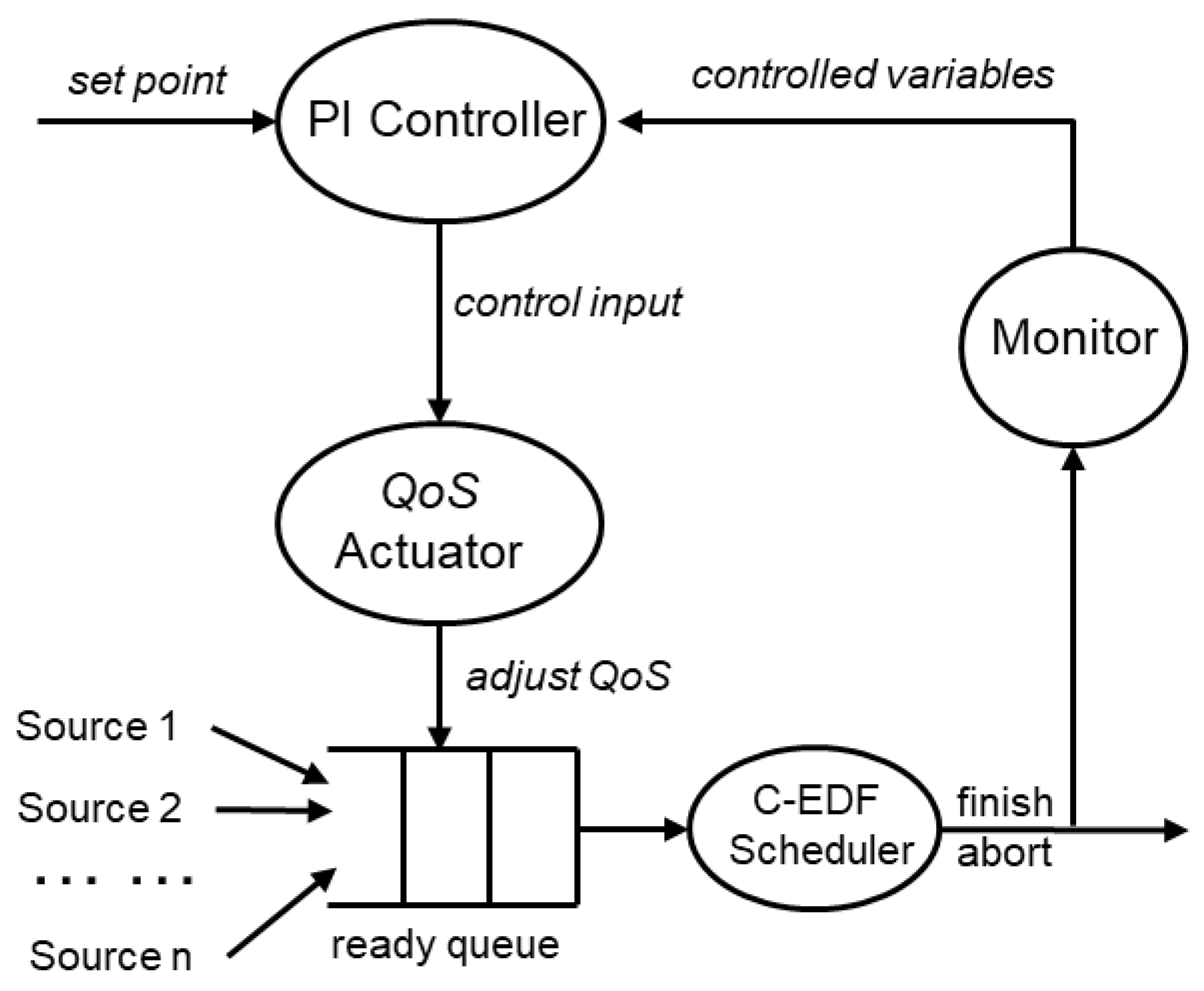
Our resource allocation architecture was modeled using a simulation framework that was implemented on a VM configured with two cores running the 32-bit Raspbian (version 10) operating system. The simulation framework was based upon the FECSIM [
25] soft real-time simulator (
Figure 4). The simulator consists of five components: a set of
Sources that are used to generate the task sets, the Scheduler that emulates the C-EDF scheduler which controls the execution of tasks; the Monitor that records the controlled variables (i.e., utilization and miss ratio); and the QoS Actuator that adjusts the QoS levels of the tasks and to perform frequency scaling (DVFS).
In order to analyze the performance of our approach, we need to model overall system utilization via load profiles. One specific load profile used in control theory is known as the step load. In terms of real-time systems, the step load represents a worst-case load variation profile. The
Step-Load defined as
jumps instantaneously from a nominal load
to a load
then stays constant after the jump. The workload used by the step-load profile is based on the task workload described in [
25]. The workload consists of a number of tasks defined by the task model described in
Section 3. Each task is defined to have four QoS levels (0.25, 0.50, 0.75, 1.0) where each level represents a percentage of the requested execution time. The estimated execution time
of task
at QoS level 3 uses a uniform distribution range [0.2, 0.8] ticks where
and
. The actual execution time is defined as
of task
at QoS level
j uses a normal distribution defined as
where the average execution time equals
with
is defined as the
execution time factor which means the estimated execution time is double the average execution time. All the QoS levels of a task
are assigned the same relative deadline
, where
is a normal distribution in the range [
1,
10]. The start time
of task
follows an exponential distribution with an average start time of
.
To analyze the performance of the feedback controller we generated a step load to stress the system. (Note: the actuator was disabled for this test so as not to bias the tuning parameters). The average CPU utilization and miss ratio are illustrated in
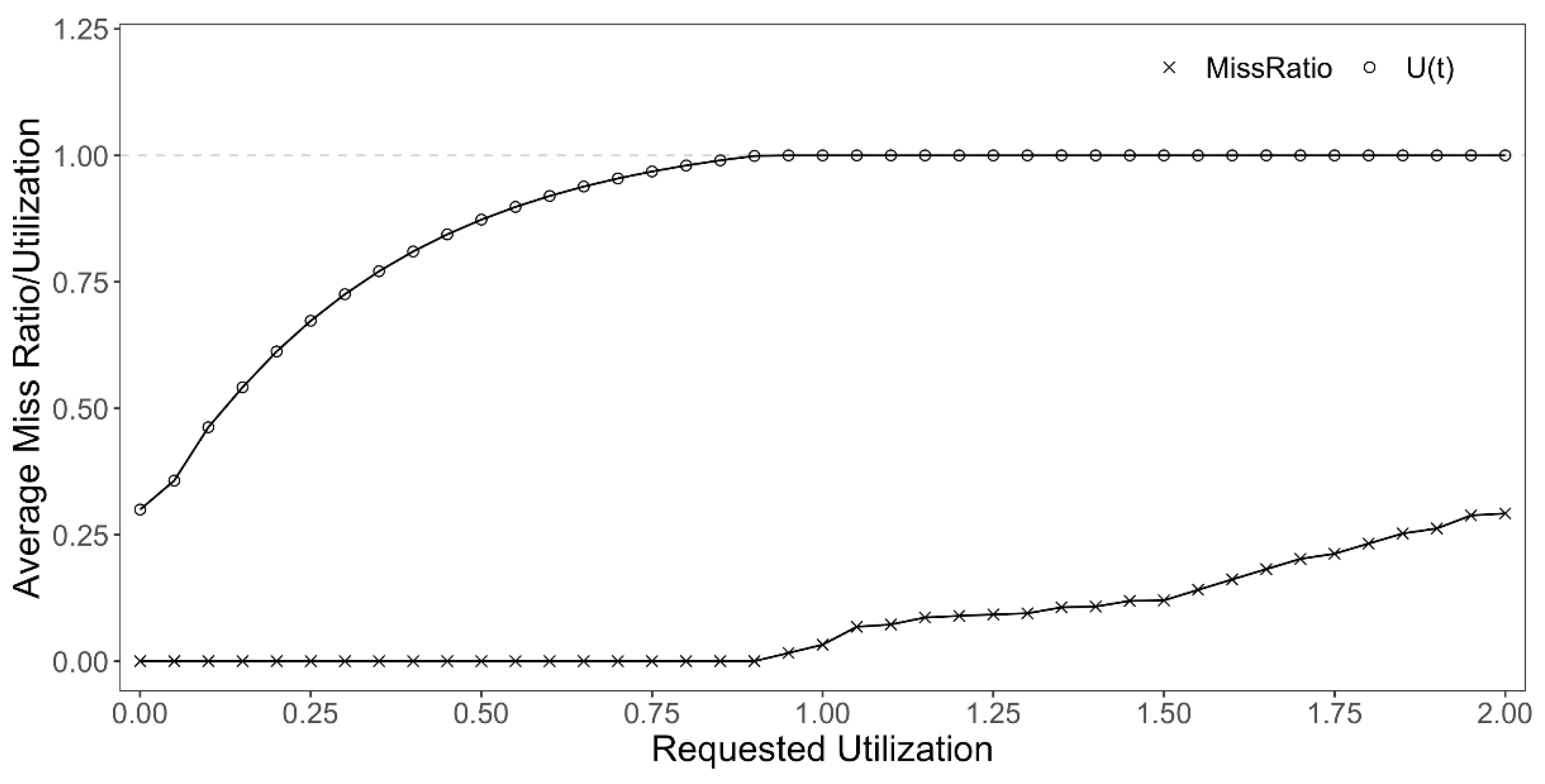
Figure 5. As shown in the graph CPU utilization is saturated at 1.0 (100%) after the utilization requested by the step load profile exceeds 100%. The miss ratio remains at zero until the requested utilization starts to exceed 90%. As a result, the demonstrated steady state performance of the controller indicates that the controller is tuned adequately.
There has been a considerable amount of work in applying feedback control mechanisms to real-time scheduling. As a result, there are a number of methods that have been applied for tuning PID-based controllers used for real-time systems. One approach is to tune the controller by running a large number of experiments that simulate the data. The issue here is that you need a large number of experiments to properly tune control parameters. Another method for tuning is to use a model that represents the real scheduling system. This is the approach that the authors in [
20] took where they used a liquid tank model of the scheduling system. A third approach adopted by the same authors and presented in a different paper [
20,
27] was to establish a baseline of the control parameters and then adjust the parameters using a simulation tool such as MATLAB. This was the same method we adopted for our approach since they used an EDF scheduler which is very similar to the C-EDF scheduler. Note: that other scheduling algorithms such as rate monotonic (RM) or deadline monotonic (DM) or even different workload characteristics could affect the control parameters which may require a re-tuning.
To evaluate the service levels and DVFS performance of QoS-EML we set the control parameters (based upon the tuning analysis done in [
20,
28]) to
for the proportional component,
for the integral component and a utilization threshold of
U(
t) = 0.30. Step Loads were applied according to
Table 1 for testing the adaptability of the system to respond to differing QoS levels.
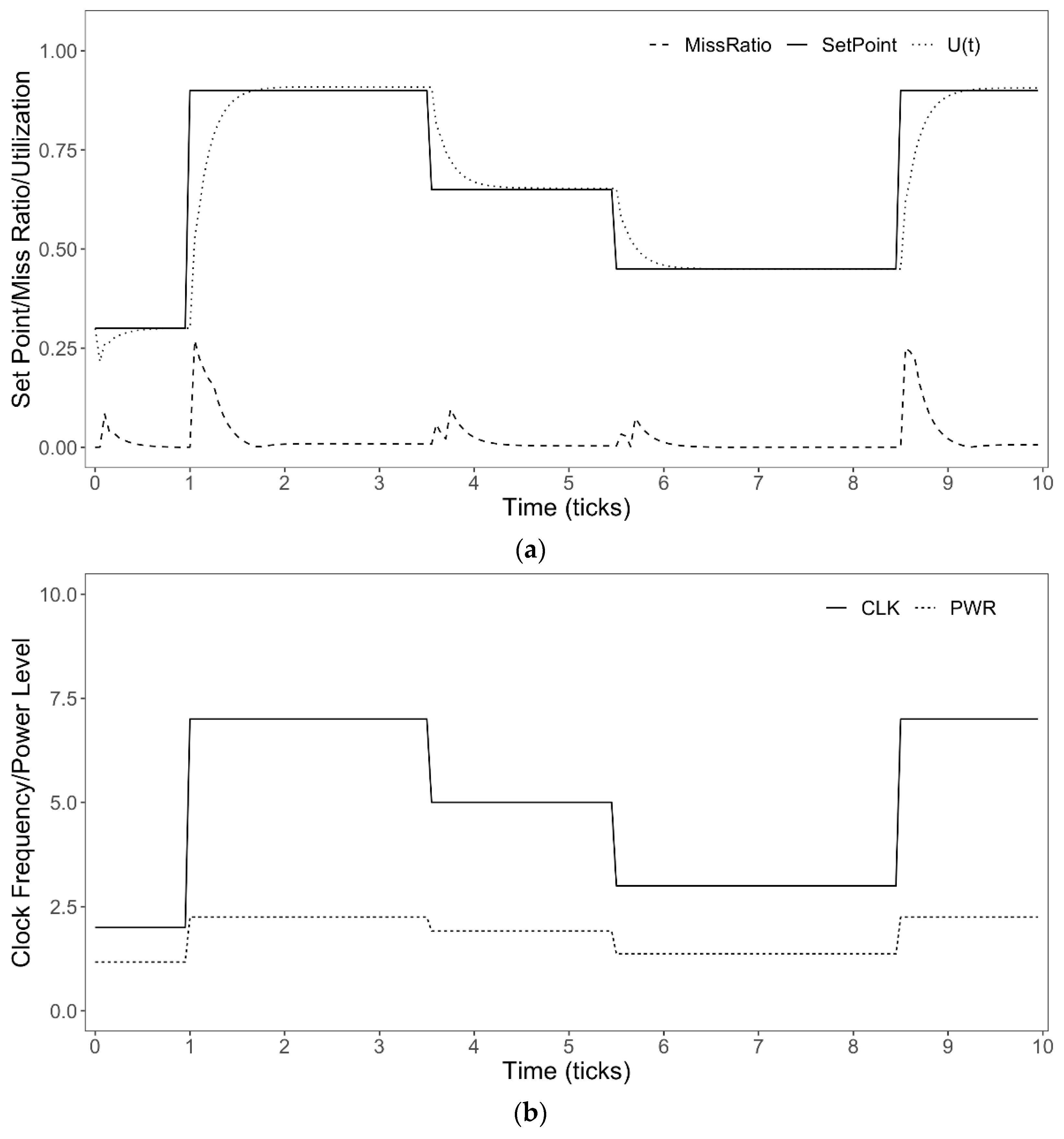
The performance of QoS-EML is illustrated in
Figure 6a as it relates to overall system utilization and task miss ratio. Notice at t = 0 the controller is activated and utilization is requested at 30% then at t = 1.0 requested utilization is increased to 90% causing missed deadlines as the QoS Actuator adjusts the execution times of the tasks to meet the threshold. The CPU utilization remains settles to a steady state around t = 1.5 and remains stable until the next Step-Load at t = 3.5 though no deadlines are missed because overall resource utilization decreases. A few deadlines are missed again at t = 8.5 as the system adjusts to the new utilization demands and then stabilizes around t = 9.0. The performance of DVFS is illustrated in
Figure 6b where the CPU frequencies are adjusted based upon the utilization reference points of the QoS Actuator. To simulate the power performance, we utilize the energy model from [
23] where dynamic power consumption is defined as:
where
C represents the capacitance of the processor, V defines the supply and
denotes the clock frequency. It is assumed that the linear increase of voltage leads to a linear increase of clock frequency applied to Equation (3) then
. The energy consumption for the task is equal to the execution time multiplied by the power consumption where,
So, to determine a baseline unit if a one-second task is set to the lowest frequency (1.0) then when the frequency of the clock is increased to 1.5× then the task will consume 2.25× more energy related to the baseline. In order to simulate the power consumption, we modeled 7 common frequency steps of the Intel Xeon E5620 Intel processor. The QoS adjustments of the power levels and clock frequency shown in
Figure 6b demonstrate that when utilization requests increase, the clock levels increase to meet increased demand as well as when demand decreases, power levels decrease accordingly.
5. Implementation
This section introduces some of the implementation details involved in getting QoS-EML running on an embedded environment. For our compute platform we used a Raspberry Pi 4, Cortex-A72 64-bit SoC running the Raspbian OS. Our resource allocation mechanism was implemented as a loadable kernel module via the standard programming interface provided by the Linux kernel. Using a loadable scheduler approach is likely the most straightforward mechanism for the prototyping of a real-time scheduler. As an example authors in [
29] utilized this approach to “pre-plant” several hooks (functions) in the original Linux scheduler. For our work, we use some of those same functions with other functions added to support multiprocessor real-time scheduling.
In order to further simplify the prototyping and testing, we leveraged the Linux Testbed for Multiprocessor Scheduling in Real-Time Systems (LITMUS
RT) [
28]. The LITMUS
RT testbed was chosen because it supports a modular plugin approach for proof-of-concept testing, provides a fairly robust set of instrumentation tools and offers a port for the Raspbian OS. In order to create a new scheduler, the code must be registered with the LITMUS
RT kernel. The code is registered as follows:
static struct sched_plugin cedf_plugin = {
.plugin_name = “C-EDF”,
.schedule = “cedf_schedule”,
.admit_task = cedf_admit_task
}
static int __init init_cedf(void ) {
return register_sched_plugin($cedf_plugin);
}
module_init(init_cedf);
The scheduler plugins for LITNUSRT require the initialization macro module_init(…) which is used by the compiler to identify the function to call during initialization. The initialization function init_cedf(…) contains the code to initialize the C-EDF scheduler. To register the scheduler plugin LITMUSRT requires a pointer to the sched_plugin structure. This structure defined as cedf_plugin(…) provides the kernel with a list of callback functions to be executed during the schedule and admit_task events. The primary list of functions used by the schedule and admit_task events is provided below:
static struct task_struct* cedf_schedule(
struct task_struct * prev);
static void cedf_finish_switch(struct task_struct *prev);
static void cedf_task_new(struct task_struct * task,
int on_rq, int is_scheduled);
static void cedf_task_wake_up(struct task_struct *task);
static void cedf_task_block(struct task_struct *task);
static void cedf_task_exit(struct task_struct * task);
static long cedf_activate_plugin(void);
static long cedf_deactivate_plugin(void);
Similar to the standard Linux loadable scheduler approach that uses the function do_fork(…) which is called when the fork() syscall is invoked LITMUSRT utilizes the following function:
static long litmus_fork(struct task_struct *task)
where task is the newly created task. Other functions that deal with QoS-based feedback are implemented in functions such as cedf_admit_task(…) and cedf_schedule (…) along with other separate helper functions such as link_task_to_cpu(…) which links a task to a CPU or preempt (…) which enforces task preemption.
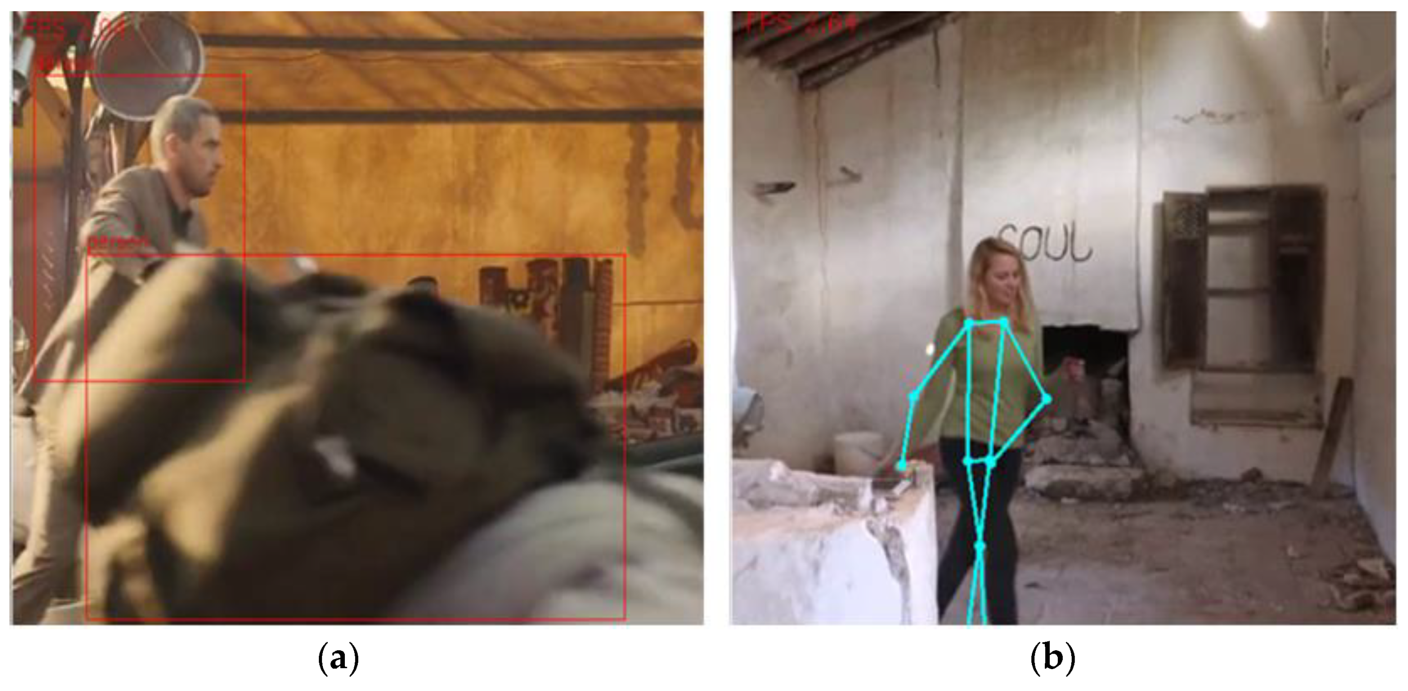
Our experiments focused on a couple of specific areas: the PI controller to limit resource saturation, the QoS actuator to be able to adjust to changing workload requirements and DVFS to be able to adjust the power consumption of the platform. The experiments were done using two different TensorFlow Lite models; an object detection model and a pose estimation model. For object detection, we used the COCO SSD MobileNet V1 model that can recognize up to 80 different objects. For pose estimation, we used the Posenet_mobileenet_v1_100_257x257 model which can recognize key features such as elbows, knees and ankles in an image.
Figure 7a provides a screenshot of the object detection model while
Figure 7b provides the screenshot for the pose detection model. Both models were provided by Q-engineering [
30].
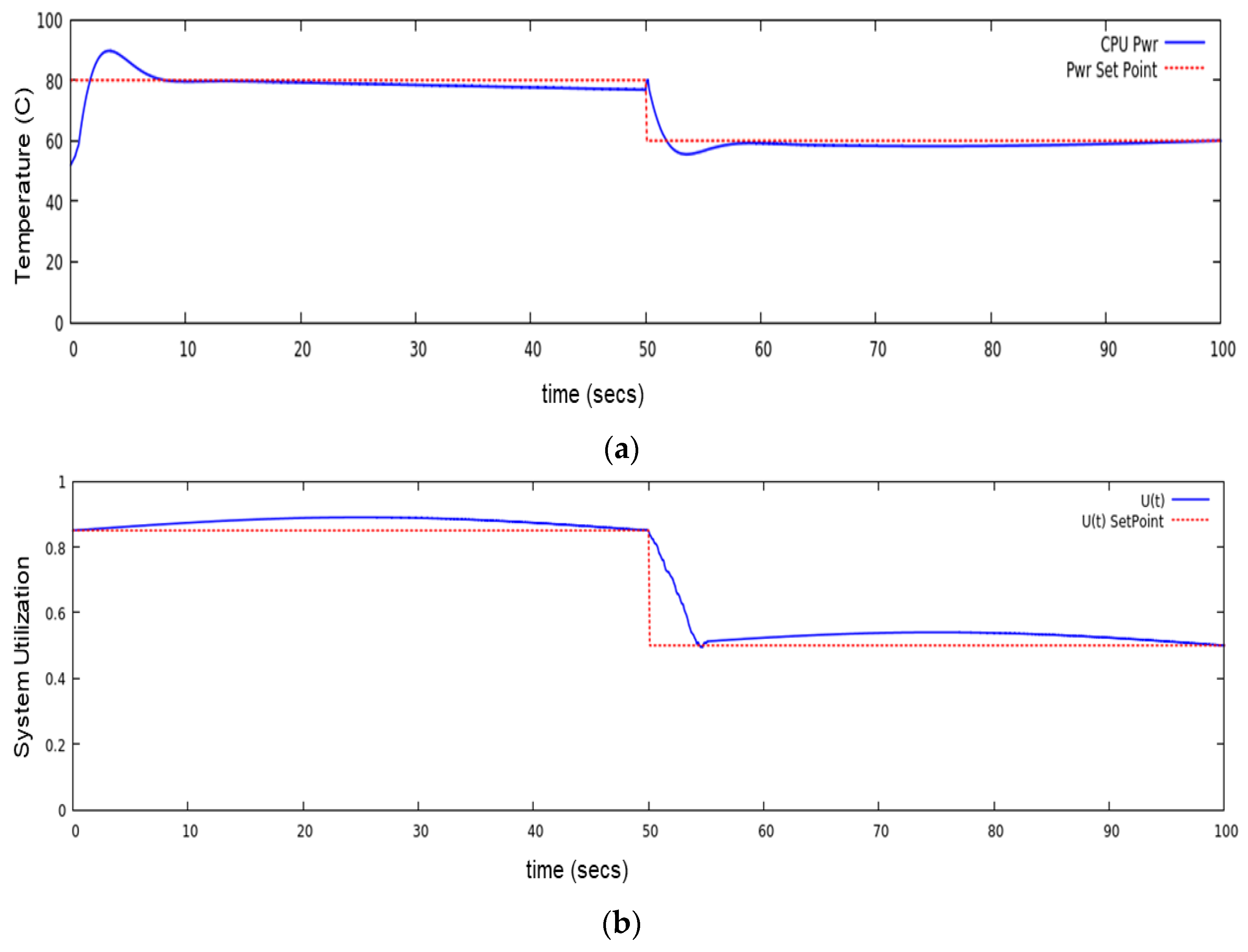
In order to verify the performance of QoS-EML we ran the two models shown above and then monitored their performance. We used
mpstat to monitor the overall system utilization and the
lm_sensors tool to monitor CPU frequency and power. As shown in
Figure 8a,b we started both the models at time 0, then at 50 s we stopped the second pose estimation model and let the object detection model run for the remaining 50 s. For the power performance, we choose a threshold of approximately 80 °C because the Raspberry Pi 4 would normally throttle back CPU performance to reduce power at that temperature (
Figure 8a). For utilization performance, we choose the set-point of 85% based on the controller performance analysis performed in the previous section. Notice how in
Figure 8b the recorded utilization stabilizes around the set-point as compared to the test run with standard Linux where the recorded utilization hovered around 95%. We did recognize that the overall utilization slightly exceeds the 85% set-point but we attribute that to other unrelated system tasks which are not currently controlled by QoS-EML.
6. Related Work
While there has been some recent research into the area of QoS for EML applications most of that work has focused on research management for network-based architectures as opposed to running on a specific target. For example, the authors in [
31] studied how the problem of resource management in a wireless network could be optimized to improve user experiences for wireless virtual reality applications. Other work [
32,
33] focused on developing a QoS model used to predict the resources that may be required for a cloud-based software service. Then, the authors incorporate a feedback loop to adjust allocated resources for the cloud software services using the QoS model to predict the necessary resources. The authors in [
34] took a slightly different approach where they applied the Genetic machine learning algorithm to optimize the resources needed by the application based upon pre-defined QoS requirements.
There is other research work related to resource allocation for embedded devices that are not necessarily focused on network-centric solutions. Researchers R. David et al. [
35] introduced a machine learning framework for running deep-learning models on resource-constrained devices. Their software framework utilized an interpreted alternative which authors claimed are more suited for embedded machine learning application as opposed to the traditional compiled approach. Named TensorFlow Lite Micro and based upon the TensorLite framework it was designed to run on embedded devices with only a few kilobytes of memory. To identify just some of the work [
36,
37,
38] there has also been a significant amount of research in designing custom hardware for machine learning applications. Known as machine learning accelerators these are customized hardware processing elements specifically designed to optimize machine learning applications. While highly effective, the problem with a customized hardware approach is that these processing elements are tightly coupled to a specific platform and cannot be applied to general-purpose embedded systems.
The general problem of allocating compute resources to embedded systems and not specifically for EML applications has been studied for years. The primary research path has been to apply QoS-based constraints to embedded real-time systems. Specifically, it’s an optimization problem in finding the allocation of tasks to resources that can satisfy some QoS requirements as well as maximize benefits. The problem is that most of this work is theoretical and only tested through simulation. Another issue is that this work is typically
a priori based resource allocation, so if any of the system parameters change then the resource allocation model has to be recalculated. However, there has been other work to apply a dynamic approach to real-time management [
39]. These dynamic approaches typically apply some type of feedback mechanism used to adapt to changes in the system. While these methods can effectively allocate tasks to resources there is no provision on how tasks are actually scheduled once they are assigned to the resource.
There has been some recent work that examines how machine learning models can be adapted to run on resource-constrained devices and the tradeoffs between hardware performance metrics, such as power, accuracy and speed. For example, authors in [
40] conducted a review of research work that focused on the use of machine learning models for Advanced Driver Assistance Systems (ADAS). Other work [
16] examined some of the design challenges involved in deploying a deep neural network onto mobile and embedded targets. Authors in this paper identified both design time and run time challenges. They concluded that custom designed DNNs could be deployed on a variety of hardware platforms to meet hardware performance constraints while runtime challenges would require an adaptive approach in order to optimize local computing resources. Our work in QoS-EML used this paper as a roadmap on how to address some of the challenges associated with running machine learning applications on embedded devices. We took both a design time and runtime approach. At design time a particular DNN model could have multiple implementations or instances where a less accurate model would use less memory and compute resources than a more accurate one. While this would require multiple instances of the same model, which would require extra storage space thus defeating the purpose of limited memory requirements, additional implementations of the same DNN model could be stored in permanent storage such as flash and only swapped in when needed. Other recent methods used to limit the memory footprint could be to employ dynamic DNNs [
18] where the model has only one implementation but multiple configurations. Depending upon the resources available applications could select a configuration that requires less or more resources depending upon the QoS requirements identified by the user. To address some of the runtime challenges we incorporated a QoS-based approach that utilized feedback to dynamically adjust to workload demands and currently available computing resources. This generic approach allowed for the same DNN model to run in a virtual machine with only minor changes to the OpenCV application as opposed to running on the actual hardware with functional accelerators (e.g., GPU). The idea is if you can tolerate the application to run slower and/or with less accuracy (e.g., QoS requirements) then the framework is generic enough to run on a wide range of embedded platforms.
7. Conclusions
In this paper, we presented a QoS-based framework that utilized feedback to solve allocation and scheduling problems with uncertainty in task workload and execution times in embedded platforms. We have shown that our proposed approach provides sufficient QoS guarantees even in the case of processor overloads as well as significant power savings as part of the DVFS algorithm in the QoS actuator. It also introduced very modest energy and latency overheads that have a limited impact on the operation and overall performance of the system. In addition to the experiments presented in this paper, the framework has also been used to explore the potential for variable rate execution of tasks where instead of having multiple instances of the same task we assign varying execution rates to the same instance based upon the user’s service level guarantees.
The work presented here can be extended in a number of ways. Currently, only aperiodic tasks are supported so periodic tasks could be incorporated. To investigate further energy savings, a dynamic power management scheme (DPM) could be examined to determine when and for how long the processor should be in an active or idle state, and could also be integrated into the scheme. The C-EDF real-time scheduler could be extended to support cooperating tasks which may need to share resources or communication. Other work could be done in determining the effectiveness of porting QoS-EML to other operating systems such as VxWorks.


