Article

Traffic Flow Prediction Based on Multi-Mode Spatial-Temporal Convolution of Mixed Hop Diffuse ODE

Department of Information Engineering, East China Jiaotong University, Nanchang 330013, China
*
Author to whom correspondence should be addressed.
Electronics 2022, 11(19), 3012; https://doi.org/10.3390/electronics11193012
Submission received: 21 July 2022 / Revised: 18 September 2022 / Accepted: 19 September 2022 / Published: 22 September 2022
(This article belongs to the Topic Intelligent Transportation Systems)

Abstract

:
In recent years, traffic flow forecasting has attracted the great attention of many researchers with increasing traffic congestion in metropolises. As a hot topic in the field of intelligent city computing, traffic flow forecasting plays a vital role, since predicting the changes in traffic flow can timely alleviate traffic congestion and reduce the occurrence of accidents by vehicle scheduling. The most difficult challenges of traffic flow prediction are the temporal feature extraction and the spatial correlation extraction of nodes. At the same time, graph neural networks (GNNs) show an excellent ability in dealing with spatial dependence. Existing works typically make use of graph neural networks (GNNs) and temporal convolutional networks (TCNs) to model spatial and temporal dependencies respectively. However, how to extract as much valid information as possible from nodes is a challenge for GNNs. Therefore, we propose a multi-mode spatial-temporal convolution of mixed hop diffuse ODE (MHODE) for modeling traffic flow prediction. First, we design an adaptive spatial-temporal convolution module that combines Gate TCN and graph convolution to capture more short-term spatial-temporal dependencies and features. Secondly, we design a mixed hop diffuse ordinary differential equation(ODE) spatial-temporal convolution module to capture long-term spatial-temporal dependencies using the receptive field of the mixed hop diffuse ODE. Finally, we design a multi spatial-temporal fusion module to integrate the different spatial-temporal dependencies extracted from two different spatial-temporal convolutions. To capture more spatial-temporal features of traffic flow, we use the multi-mode spatial-temporal fusion module to get more abundant traffic features by considering short-term and long-term two different features. The experimental results on two public traffic datasets (METR-LA and PEMS-BAY) demonstrate that our proposed algorithm performs better than the existing methods in most of cases.

1. Introduction

Spatial-temporal prediction has large-scale applications in our daily life, such as traffic flow prediction [1,2,3], climate prediction [4,5], earthquake prediction [6,7], etc. Accurate spatial-temporal prediction plays an important role in improving the quality of service for these applications. In this paper, we study one of the most representative spatial-temporal forecastings, traffic flow forecasting, which is a key part of Intelligent Transportation Systems (ITS). Traffic flow forecasting attempts to predict future traffic flow by given historical traffic conditions and the basic road network. As ITS continues to develop, the scale and dimensionality of spatial-temporal data collected by road sensors become larger and larger, serving as data support in the field of traffic flow forecasting. Traffic flow forecasting aims at modeling dynamic changes in traffic flow is a well-researched spatial-temporal forecasting problem, of which multi-step traffic flow forecasting is a key task. Traffic flow forecasting has a wide range of applications. Not only can it help travelers plan their routes, but it can also provide insightful information for active traffic management strategies to improve traffic efficiency and safety.
At present, deep learning models are widely used for traffic flow prediction and applied to intelligent transportation systems, and many deep learning models have been proposed for traffic speed prediction. According to the specific modeling strategy, the state-of-the-art deep learning models can be divided into three categories: grid-based, graph-based, and multivariate time-series models [8]. However, previous approaches using convolutional neural networks (CNNs) [9,10] and recurrent neural networks (RNNs) [11] only deal with grid structures (e.g., images and videos) and ignore non-Euclidean correlations determined by complex road networks. To address this problem, recent studies on spatial-temporal graph modeling have formulated traffic flow prediction as a graph modeling problem. Graph neural networks (GNNs) are used to capture the spatial correlations in traffic networks, while time series models capture temporal correlations. In particular, they have shown effectiveness in integrating graph convolution and temporal convolution into models to extract spatial-temporal features. Now the most popular graph convolution neural networks are graph convolution network(GCN) [12,13], graph attention networks (GAT) [13,14], and graph diffusion networks [15]. Compared to traditional time series and machine learning methods, deep learning models can flexibly handle relatively long time series and large traffic network structures. However, many existing methods encounter some major problems.
  • Neural networks typically perform better when stacking with more layers, while GNNs benefit little from depth. Ordinary GNNs have been shown to suffer from over-smoothing [16], with the increase in the number of layers of the graph convolution network, the features of all nodes tend to be more and more consistent.
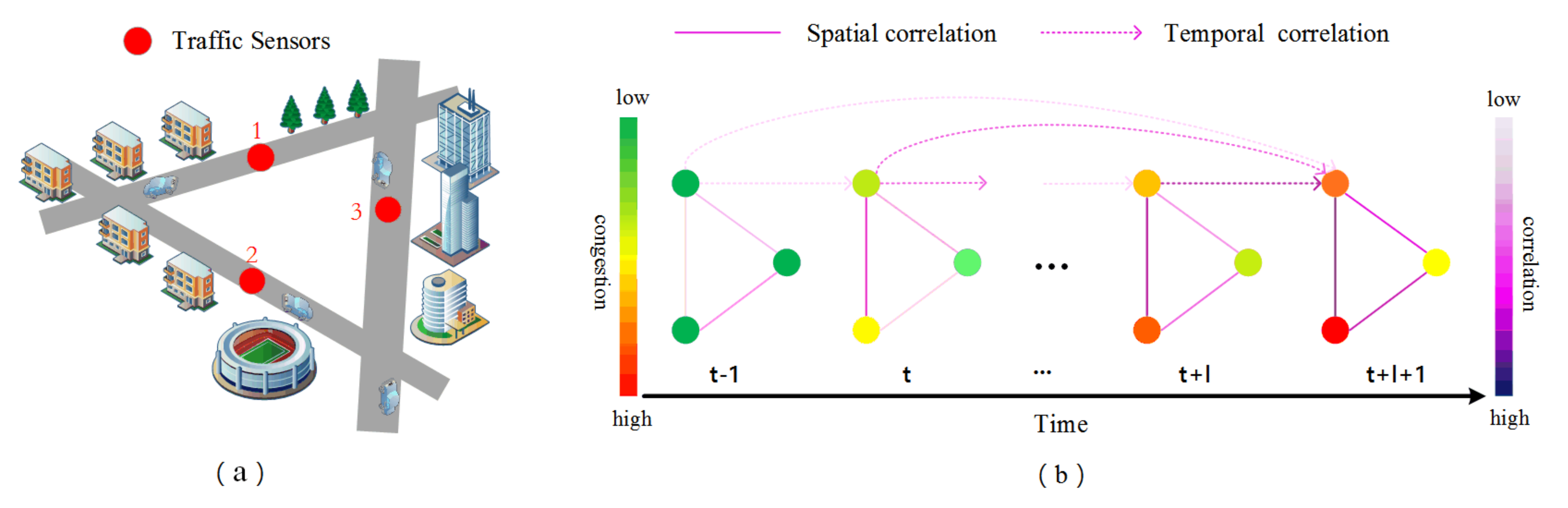
  • The traffic flow in a traffic network is dynamic over time. For most areas in the road network, the traffic flow in a given time slice may be affected by the traffic flow in different historical periods, which makes the long-term flow dependence more complex, resulting in low prediction accuracy for a long time. As shown in Figure 1b traffic map signal tensor, the different colors of the sensors represent the level of congestion on the road. The sensor lines represent the correlation of the roads, the solid lines represent the spatial correlation of the roads and the dashed lines represent the correlation of the traffic at different time moments. The different colors of the sensor lines represent the degree of correlation between the roads. The congestion states of Road 1, Road 2, and Road 3 vary over time at different moments, which are both cyclical and subject to uncertainty in the long and short term. The short-term is affected by the timing of emergencies (e.g., sudden car accidents) and the long-term is affected by the time cycle (e.g., commuting), and the simultaneous long and short term makes the final traffic flow prediction tricky.
  • In long-term forecasting, there is a lot of redundant information and hidden spatial dependencies in the traffic road network, which makes forecasting the future traffic flow very challenging. For example, in Figure 1a, the structure of the traffic road network, sensor 1 represents a road with residential areas and forested areas, sensor 2 represents a road with residential areas and stadiums, while sensor 3 represents a road with supermarkets and office buildings, while we cannot simply determine the relevance of roads by the difference in areas, and also the same road structure in different areas will show different spatial dependencies (the factors affecting these are economy, population, culture, etc.). This redundant information makes the spatial relevance of roads complex and varied.
To address the existing challenges, we propose a new deep learning framework called spatial-temporal convolution of mixed hop diffuse ODE. First, we use adaptive spatial-temporal convolution to extract the spatial-temporal dependence of traffic in short time steps. At the same time, the more extensive receptive fields in the ODE spatial-temporal convolution module enable to capture of the dependence features in longer time steps. Finally, fusing the features of two different spatial-temporal convolution modules enables the capture of more hidden spatial-temporal dependencies in the traffic. Graph Wavenet [17] uses a self-adaptive adjacency matrix to extract global features, but this method weakens the extraction of long-term features. Different from GraphWavenet, our proposed method use ODE to improve long-term feature extraction. Similar to STGODE [16], our proposed method uses ordinary differential equations. However, different from STGODE, MHODE improves the ODE with a mixed hop diffuse layer that can improve long-time feature extraction. In addition, MHODE is able to extract short-term and long-term features separately and uses a multi-mode fusion mechanism to obtain more abundant features to improve the prediction effect.
We evaluated MHODE on two public transport network datasets and MHODE can achieve satisfactory performance. The main contributions of this work are as follows:
  • We propose an adaptive spatial-temporal convolution module that can extract the spatial-temporal features of traffic flow in short time steps using Gate TCN and adaptive graph convolution;
  • We propose a spatial-temporal convolution module based on mixed hop diffuse ODE that uses the wider receptive field of the ODE graph convolution to extract new features while the mixed hop diffusion layer retains some of the original features and preventing transition smoothing, thereby extracting more spatial features over a longer time domain;
  • We propose a new multi-mode spatial-temporal fusion module to integrate the hidden relationships between traffic data. We fuse the extracted features from different graph convolutions and can extract more hidden spatial-temporal dependencies;
  • We evaluated our proposed model on two traffic datasets and conducted a large number of comparative experiments. The experimental results show that the MHODE performs better than other models in both datasets.

2. Related Work

In recent years, traffic flow prediction has become a hot topic in ITS and has received wide attention. In this section, we briefly review the traditional statistical-based and deep learning-based methods used for traffic flow prediction.

2.1. Traffic Flow Forecasting Based on Statistical Methods

Traffic flow forecasting plays a crucial role in ITS. Accurate traffic flow forecasting can assist in route planning, guide vehicle scheduling and alleviate traffic congestion by vehicle scheduling [18]. Statistical methods usually establish a series of stationary assumptions for traffic flow, and then establish mathematical equations to predict traffic flow. Such traffic flow forecasting methods commonly include moving average forecasting models (HA), and differentially integrated moving average autoregressive models (ARIMA). Williams et al. [19] used the average of all historical data to predict traffic values for future time intervals. Alghamdi et al. [20] proposed a differentially integrated moving average autoregressive model (ARIMA) and extended a series of linear models based on ARIMA, including autoregressive (AR), moving average (MA), and autoregressive moving average (ARMA), of which (ARIMA) [20] and Kalman filtering [21] are now widely used in traffic flow forecasting. The vector autoregressive model VAR [22] is a more advanced time series forecasting model that improves the accuracy of traffic forecasting by capturing the relationship between all traffic flows. However, traditional methods are often based on certain smoothing assumptions and are computationally intensive and difficult to achieve high forecasting accuracy. They also ignore spatial dependence and are based only on the assumption of time series smoothness, which makes it difficult to take into account the dynamic changes in traffic conditions.

2.2. Traffic Flow Forecasting Based on Deep Learning Methods

In recent years, with the rapid development of deep learning neural networks, more and more researchers are applying deep learning techniques to the field of traffic flow prediction. By building deep neural network structures, deep learning models can tap into more non-linear features in traffic flow. The common traffic flow prediction methods in the field of deep learning are currently Recurrent Neural Network (RNN) based methods and Graph Neural Network (GNN) based methods.
RNN-based approaches: Traffic flow data is a classical type of time-series data, and historical traffic flow often has an important impact on future traffic flow. As a favorable tool for processing time-series data, recurrent neural networks (RNNs) have been widely noted in the field of traffic flow forecasting, such as deeply stacked bidirectional and unidirectional LSTM recurrent neural networks [10] and gate recurrent units (GRUs) [23] has also been used to explore the temporal features of traffic data. The main drawback of RNN-based approaches is that it becomes inefficient for long sequences and their gradients are more likely to explode when they are combined with graph convolutional networks. However, based on recurrent neural network approaches tend to process traffic data in the form of grid pictures, which is only adapted to deal with non-Euclidean distance data, and it is difficult to capture the spatial dependence of traffic in non-Euclidean distance data like traffic road network traffic.
GNN-based approaches: Traffic data is a classical non-Euclidean structured graph data, which can be better represented as non-Euclidean distance data. Graph neural network approaches show great potential for capturing the spatial dependence of vertices in a graph. Traffic speed prediction is a well-defined and representative geometric spatial-temporal learning problem that encodes each road segment as a node in the graph, with the edges between the nodes corresponding to the spatial influence of the road segment. many methods have been proposed for traffic speed prediction. Yu et al. [24] proposed a spatial-temporal graph convolutional neural network (STGCN), which used a CNN-based approach that combines a GCN layer with a 1D convolutional layer. Li et al. [25] designed a diffusion convolutional recurrent neural network (DCRNN), which proposed an encoder-decoder architecture that treats traffic flow as a diffusion. Wu et al. [17] proposed deep spatial-temporal modeling (GraphWavenet), which used graph convolution to adjust the adaptive dependency matrix by learning node embeddings in the spatial domain and one-dimensional convolution in the temporal axis by a stacked expansion of 1D Convolution operations improve on STGCN [24]. They process graphical information and time series separately, building a model with a complete convolutional structure in both spatial and temporal views, resulting in faster training with fewer parameters. Multi-interval attention bi-component graph convolutional network (MRA-BGCN) [26] uses bi-component graph convolution to model node and edge correlations. GMAN [27] is a graph multi-attention network that uses a spatial-temporal attention mechanism and a gate mechanism to fuse complex spatial-temporal correlations. ST-GRAT [28] uses node attention operations to handle spatial dependencies between traffic sensors and temporal attention to consider temporal dependencies.
For previous graph spatial-temporal models, their GNNs are limited in capturing hidden spatial dependencies, making it difficult to capture both long-term and short-term traffic dependencies, which leads to poor prediction results. At the same time, previous methods tend to extract only one spatial dependency using a single graph convolution, failing to capture more hidden spatial dependencies, while often being less effective for feature extraction on long-time steps.

3. Preliminary

Referring to GraphWavenet [17] and STOGDE [16], we introduce the definitions of Traffic network, Graph signal tensor, and Traffic flow forecasting in this chapter.
Definition 1.
(Traffic network G) As shown in Figure 1a, we represent the road network as a graph. For the graph G = V , E , A , where V is the set of nodes representing the traffic sensors on the road network (e.g., the red dots labeled 1, 2, 3 in Figure 1a); E is a set of edges representing the connectivity between vertices; the adjacency matrix derived from the graph is denoted as A R N × N is the weighted adjacency matrix, where A v i , v j denotes the proximity (measured as road network distance) between the vertices v i and v j . We use a Gaussian threshold kernel function [25] to construct the adjacency matrix of the traffic road network graph, and the construction process can be expressed as
A v i , v j = exp d i s t v i , v j 2 σ 2 , d i s t v i , v j K 0 , o t h e r w i s e ,
where A v i , v j represents the edge weight between sensor v i and sensor v j , d i s t v i , v j represents the distance of the road network from sensor v i to sensor v j . σ is the standard deviation of the distance and κ is the threshold value.
Definition 2.
(Graph signal tensor χ) As shown in Figure 1b, we use x t i R F , i = 1 , 2 , , N to represent the data of node v i at time t. F is the dimension of the input feature (in our experiments, it consists of two features: outflow and inflow, i.e., d = 2 ). X t = x t 1 , x t 2 , , x t N R N × F denotes the observation of all nodes at time t. χ = x 1 , x 2 , , x t R N × F × T denotes the observations of all nodes at all times.
Definition 3.
(Traffic flow forecasting) The goal of traffic flow forecasting is to learn a mapping function from historical features to predict traffic values at future moments X = x T + t 1 , x T + t 2 , , x T + t p , given the tensor of observations at N vertices of the historical p time steps observed on the traffic network G, to predict traffic values at q future time steps, the mapping relationship is expressed as follows:
x T + t 1 , x T + t 2 , , x T + t p , G f x T + t p + 1 , x T + t p + 2 , , x T + t p + t q ,
where X T + t 1 : T + t p = x T + t 1 , x T + t 2 , , x T + t p R N × F × p , and X T + t p + 1 : T + t p + t q = x T + t p + 1 , x T + t p + 2 , , x T + t p + t q R N × F × q .

4. Model

In this section, we first outline the general architecture of the multi-mode spatial-temporal convolution of mixed hop diffuse ODE. Then, we introduce the structures of the adaptive spatial-temporal convolution module and the mixed hop diffuse ODE spatial-temporal convolution module. Finally, we present the multi-mode spatial-temporal fusion module.

4.1. General Framework

We show the general framework in Figure 2. It consists of stacked spatial-temporal layers and an output layer. The spatial-temporal layers consist of two paths processed in parallel, respectively. In Figure 2, module-A is the adaptive spatial-temporal convolution layer, consisting of the self-adaptive adjacency matrix graph convolution layer (Self-adaptive adjacency matrix GCN) and the gate temporal convolution layer in Figure 3 (Gate TCN), which consists of two parallel temporal convolution layers (TCN-a and TCN-b). In Figure 2, module-B is a mixed hop diffuse ODE spatial-temporal convolution module, consisting of a mixed hop diffuse ODE graph convolution network (ODEGCN) and a temporal convolution layer (TCN). After two different graph convolution spatial-temporal modules, the multi-mode spatial-temporal fusion module is used to fuse the spatial dependencies extracted from the different spatial-temporal modules to obtain more hidden spatial-temporal dependencies.

4.2. Adaptive Spatial-Temporal Convolution Module

As shown in module-A of Figure 2, the adaptive spatial-temporal convolution module consists of two parts: Gate TCN, and adaptive adjacency matrix graph convolution, aiming to learn global temporal features and global spatial features of the data respectively. Details are as follows.
Gate TCN: Temporal Convolutional Network (TCN) is a common model used in temporal data. We use dilation causal convolution [29] as our temporal convolution layer (TCN) to capture the temporal trends of nodes, which helps parallelize computation and alleviate the gradient explosion problem. The receptive field of the model grows exponentially by stacking dilation causal convolution layers with dilation factors in increasing order. It allows the expanded causal convolutional network to capture longer sequences with fewer layers, thus saving computational resources. As shown in Figure 3, we use a temporal convolutional layer (Gate TCN) combined with a gate mechanism to capture the temporal trend of the nodes. A simple Gate TCN contains only one output gate. Given an input X R N × T × F , it takes the form
H g t c n = tanh Θ 1 × X σ Θ 2 × X ,
where H g t c n R N × T × F is the output of the Gate TCN, Θ 1 and Θ 2 are the learnable parameters of the convolution filter, ⊙ is the element product, σ · is the sigmoid activation function, and × is the null convolution operation.
Adaptive adjacency matrix graph convolution: considering the structural information of the nodes and graph convolution is a necessary operation for extracting node features. The graph convolution module aims to fuse the information of nodes and their neighbors to deal with the spatial dependence in the graph. We use the ReLU activation function to eliminate weak connections. The SoftMax function is used to normalize the adaptive adjacency matrix. The normalized adaptive adjacency matrix can therefore be considered as a transfer matrix for the hidden diffusion process. By combining the predefined spatial dependencies with the self-learning hidden graph dependencies, we use the following graph convolution layers:
H s g c n = k = 0 K P f k H g t c n W k 1 + P b k H g t c n W k 2 + A a p t k H g t c n W k 3 ,
where H s g c n R N × T × F is the output of the convolution of a graph of ODE, P k represents the power of the transfer matrix, in the case of directed graphs the diffusion process has two directions, forward and backward, P f = A A r o w s u m A r o w s u m A represents the forward transfer matrix, P b = A A r o w s u m A T r o w s u m A T represents the backward transfer matrix, A is the weighted adjacency matrix, and H g t c n R N × T × F is the output of the Gate TCN, in this part is the input. A a p t k is the adaptive adjacency matrix, which does not require any prior knowledge and is learned end-to-end by stochastic gradient descent. In this process, the model is allowed to study hidden spatial dependencies. This is achieved by randomly initializing two dictionaries with learnable parameters E 1 , E 2 R N × c . The adaptive adjacency matrix is
A a p t k = S o f t M a x Re L U E 1 E 2 T ,
where E 1 is the source node embedding and E 2 is the target node embedding. By multiplying E 1 and E 2 , we derive the spatial dependency weights between the source and target nodes.

4.3. Mixed Hop Diffuse ODE Spatial-Temporal Convolution Module

As shown in module-B of Figure 2, the mixed hop diffuse ODE spatial-temporal convolution module consists of two parts: Residual TCN, and mixed hop diffuse ODE graph convolution, which aims to learn local temporal features, and local spatial features of regional data respectively. Details are as follows.
Residual TCN: In module-B of Figure 2, in order to improve the performance of extracting long-term temporal dependence, a one-dimensional dilated temporal convolutional network along the time axis is used here. The flow rate of a time slice is highly correlated with its historical state. As shown in module-B in Figure 2, we use temporal convolutional layers given the speed and simplicity of training. By adding dilation factors to stack the dilation convolutional layers, the receptive field of the model grows exponentially. Moreover, compared with recurrent neural networks, the dilation convolution layers can be computed in parallel, thus alleviating the gradient explosion problem and greatly reducing the time complexity. At the same time, a residual structure is added to enhance the convolutional performance, and the temporal convolutional layers take the form of
H r t c n l = σ Θ 3 * H r t c n l 1 ,
the input to the first layer is the raw traffic data, i.e., when l equals 1, H r t c n l = X , where X R N × T × F is the input to the Residual TCN, H r t c n l R N × T × F is the output of the l layer of the Residual TCN, σ · is the sigmoid function, and Θ 3 is the learnable parameters of the convolutional filter.
Mixed hop fusion ODE graph convolution: Conventional GCNs usually encounter the over-smoothing problem, so Fang et al. [16] proposed a STOGDE to improve the conventional GCN using an ordinary differential equation (ODE). The new GCN in this paper takes the form of
H o de l = i = 0 l H r t c n × 1 A i × 2 U i × 3 W i ,
where H o de l R N × T × F represents the output of the ordinary differential graph convolution at layer l, H r t c n R N × T × F represents the output of the residual time convolution, in this part the input to the ordinary differential equation graph convolution, A R N × N is the weighted adjacency matrix, the time dimensional fully connected parameter U R T × T , and the feature dimensional fully connected parameter W R F × F . It can be seen that the final output will have information from each layer of the GCN without losing much information. This is simplified by Fang et al. [16] due to the number of parameters, where Fang et al. [16] first used the continuous variable t to replace n in the Equation (6) and treated the equation as a Riemann sum from 0 to n, which denotes
H o d e = i = 0 n H r t c n × 1 A i × 2 U i × 3 W i .
The following equation is obtained after further derivation of the integral of Equation (7). We can see STOGDE [16] for details of the solution procedure,
d H o de t d t = H o de t × 1 ln A + H o de t × 2 ln U + H o de t × 3 ln W + c o n s t ,
substitute Equation (8) into the O D E S o l v e . A STGODE learning framework is then obtained as follows:
H o d e t = O D E S o l v e d H o d e t d t , H r t c n , t ,
the information propagation step recursively propagates the node information as well as the given graph structure. However, a serious limitation of graph convolutional networks is that as the number of graph convolutional layers tends to infinity, the node hidden states converge to a single point. This is because graph convolutional networks with multiple layers reach the limit of the random wandering distribution, regardless of the initial node state. To address the over-smooth, We use the theory proposed by Klicpera et al. [30], we retain a portion of the original states of the nodes during propagation so that the propagated node states can both remain local and explore deep neighborhoods. Therefore we propose a new ODE learning framework,
H m h o d e t = O D E S o l v e d H o d e t d t , H r t c n , t × α + 1 α × H r t c n ,
where α is the retention factor, which determines how much of the original state information is retained, and we will analyze this parameter specifically in the parametric analysis in Section 5.

4.4. Multi-Mode Spatial-Temporal Fusion Module

Deep learning methods have attracted a great deal of interest in recent years due to the highly non-linear and complex nature of traffic data. However, few methods can satisfy both long-term and short-term forecasting tasks. In contrast, the multi-mode spatial-temporal fusion module is a fusion of features extracted from the adaptive spatial-temporal map convolution module and the mixed hop diffuse ordinary differential equation spatial-temporal convolution module. The short-term spatial-temporal features are fused with the long-term spatial-temporal features to achieve simultaneous optimization of both long-term and short-term prediction tasks,
H o u t = H m h o d e + H s g c n + X ,
where H o u t R N × T × F is the output of the multi-mode spatial-temporal fusion module, H o d e R N × T × F is the output of the mixed hop ODE spatial-temporal convolution module, H s g c n R N × T × F is the output of the adaptive spatial-temporal map convolution module, and X R N × T × F is the original input. The residual joint is used in this module to enable better fusion of features from the upper module and avoid feature conflicts.

5. Experiments

In this section, we elaborate on the experimental details in terms of datasets, parameter settings, evaluation metrics, analysis of experimental results, and ablation experiments to validate the effectiveness of our proposed algorithm.

5.1. Datasets and Pre-Processing

We validated MHODE on two public transportation network datasets (METR-LA and PEMS-BAY), published by Li et al. [25] METR-LA records four months of traffic speed statistics from 207 sensors on Los Angeles County motorways, with details of the experimental data shown in Table 1. PEMS-BAY is the traffic data collected by the California Department of Transportation’s Performance Measurement System, which includes six months of traffic speed information from 325 sensors in the Bay Area were included. We used the same data pre-processing procedure as in Li et al. [25]. Observations in the sensors were used in 5-min time steps to construct the experimental input data. The raw input data were normalized using the Z-Score normalization method before model training. The datasets were divided chronologically, with 70% used for training, 10% for validation, and 20% for testing. Table 1 provides a detailed description of the experimental datasets.

5.2. Experimental Setup

To cover the length of the input sequence, we use 8 layers of spatial-temporal convolution, with a sequence of expansion factors for each layer (i.e., the expansion rate) of 1, 2, 1, 2, 1, 2, 1, 2. We use Equations (3) and (8) as the iterative update method for each graph convolution layer, with a diffusion step of K = 2. We randomly initialize the node embeddings by a uniform distribution of dimension 10. We train MHODE using the Adam optimizer with an initial learning rate of 0.001. A Dropout of p = 0.3 is applied to the output of the graph convolution layer. The metrics we chose to evaluate included mean absolute error (MAE), root mean square error (RMSE), and mean absolute percentage error (MAPE). Missing values were excluded from training and testing, and all tests used 60 min as the historical time window, i.e., 12 observed data points (t = 12) were used to predict traffic flow for the next 15, 30, 45, and 60 min (Tp = 3, 6, 9, 12).

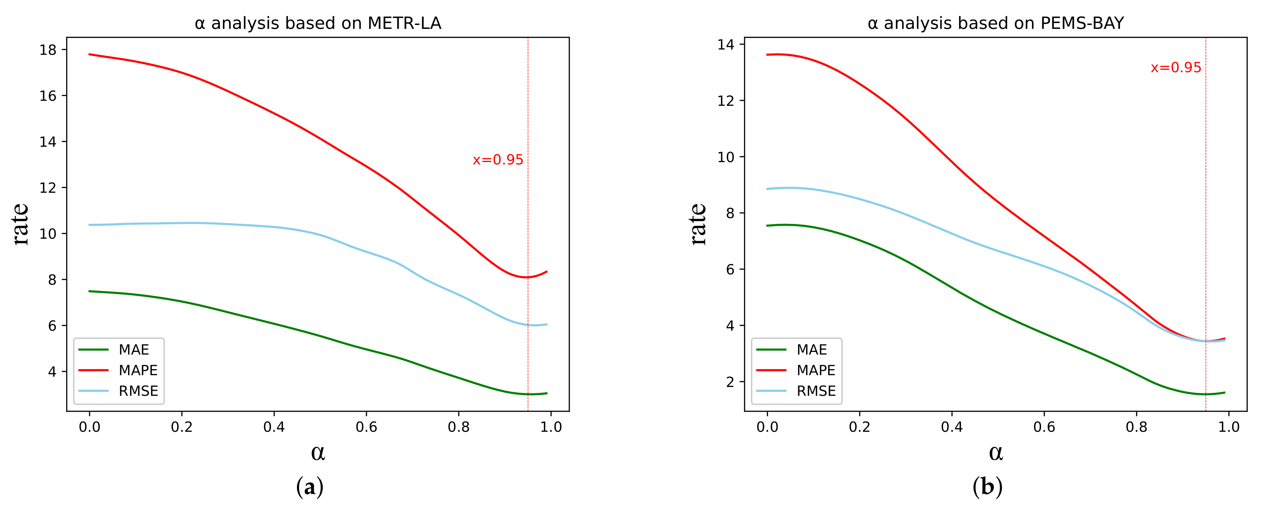
5.3. Hyperparametric Studies

To further study the effect of the retention coefficient on the experimental results in the spatial-temporal convolution module of the mixed hop diffuse ODE, we set different α values in the two datasets to achieve the best prediction accuracy of the model by selecting the optimal. The error of the model was observed in the experiment by incrementing 0.1 from 0 to 1. The experimental results are shown in Figure 4. Figure 4a,b show the experimental results on the METR-LA dataset and the PEMS-BAY dataset respectively. From the figures, we can see that on both datasets, optimal results are obtained for all three evaluation metrics when α is taken around 0.95. Combined with Table 2, we can see more clearly that the three evaluation metrics outperform the other values when α = 0.95 is taken. The possible reason for this result is that when α = 0.95 , the original state information of the root node has a negative impact on the long-range spatial information but can improve the near-range spatial information, while the inherent disadvantage of the ODE is that the extraction of short-range spatial information is not satisfactory. The model can be improved by retaining part of the original root node information. At the same time, the addition of the original root node information can contribute to the prevention of smoothing in the model. The results for both cases show that it is effective for us to add a mixed hop diffuse layer to the convolution of the ordinary differential equation map.

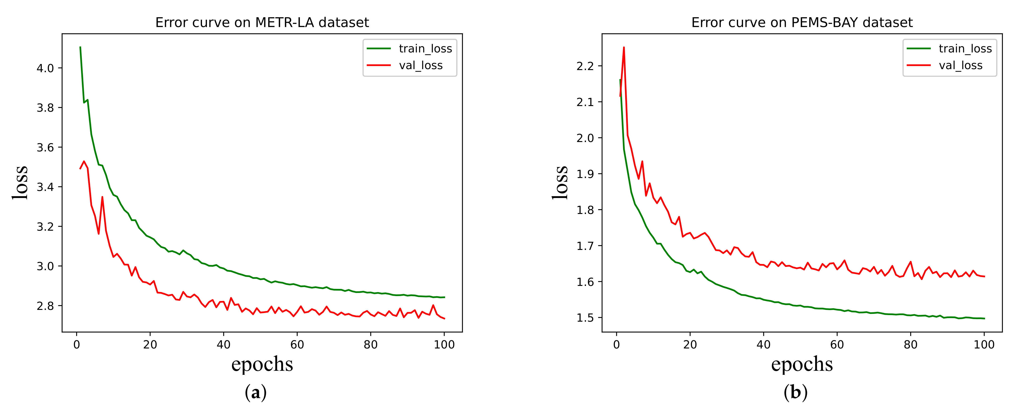
5.4. Convergence Analysis

To explore the final convergence of the model, we show the error of the model training process. Figure 5a,b show the error profiles of the model training and validation process on the METR-LA dataset and PEMS-BAY dataset respectively. The X-axis in the Figure 5 represents the number of training epochs and the Y-axis represents the model training loss and validation loss. After about 80 epochs, the error curve is stable and does not change drastically, indicating that the training has reached convergence. A similar trend occurs during the validation process. Until finally convergence is reached, it means that the model is not overfitted during the training process.

5.5. Performance Comparison

DCRNN [25]: A diffusion convolutional recurrent neural network which combines diffusion map convolution and recurrent neural networks.
STGCN [24]: A spatial-temporal graph convolution network that combines graph convolution and one-dimensional convolution.
Graph Wavenet [17]: A spatial-temporal graph convolutional network that integrates diffusion graph convolution and one-dimensional expansion convolution.
ST-MetaNet [31]: A sequence-to-sequence architecture that uses meta-networks to generate parameters.
MRA-BGCN [26]: A multi-range of attention two-component GCN.
FC-GAGA [32]: A hard graph gate mechanism for traffic flow prediction.
GMAN [27]: Graph multi-attention network with spatial and temporal attention.
MTGNN [12]: A spatial-temporal network for generating one-way adaptive graphs using external features.
ST-GRAT [28]: An attention-based traffic flow prediction framework. The framework mainly consists of spatial attention, temporal attention, and spatial forward vectors.
Notably, our model obtains satisfactory results for 60-min predictions on both datasets, a result that demonstrates the competitive advantage of MHODE for long-term predictions. Compared to other spatial-temporal models, MHODE outperforms the previous convolution-based approach STGCN and outperforms the loop-based approach DCRNN. This reason may be that convolution-based approaches are less able to capture more spatial dependencies, whereas our multigraph convolution can capture more hidden spatial dependencies and features, thus improving the prediction results. The second best model suggested in Table 3, GMAN, this model uses graph attention to make it very good at long time prediction, but performs poorly in short time prediction, whereas MHODE is essentially similar to GMAN in the 60-min range; however, we maintain better performance at short time prediction in the same situation, with 15-min prediction results for our model’s MAE, RMSE and MAPE are 4.3%, 6.8% and 7.4% lower respectively compared to GMAN. This may be because our ordinary differential equation spatial-temporal module can capture more of the long-term dependencies in the long sensory field of the middle graph convolution, while our adaptive spatial-temporal convolution module can capture the spatial-temporal dependencies in the short time step. This enables us to achieve satisfactory prediction results in short time steps while ensuring long time prediction.

5.6. Ablation Experiments

In our experiments, we conducted ablation experiments on our proposed model by removing or changing some modules. Specifically, MHODE has three variants: (1) No Ordinary Differential Equation GCN (NODEGCN): i.e., the Ordinary Differential Equation spatial-temporal Convolution module is removed and only the self-adaptive spatial-temporal Convolution module is used to extract the spatial-temporal features of the traffic. (2) No self-adaptive Adjacency Matrix GCN (NSGCN): i.e., the adaptive spatial-temporal convolution module is removed and only the ODE spatial-temporal convolution module is used to extract the spatial-temporal features. (3) No mixed hop diffuse Layer (NMHP): the mixed hop layer is removed in the ODE spatial-temporal convolution module. We conducted experiments on the above three variants at different prediction time steps and the results are shown in Figure 6 and Figure 7. Figure 6 shows the experiments for the variant on METR-LA and Figure 7 shows the experiments for the variant on PEMS-BAY. We show the results for three specific time steps: the third time step (15 min), the sixth time step (30 min), and the twelfth time step (60 min). As we can see from the figures, compared with NODEGCN, the MAE of our model on datasets METR-LA and PEMS-BAY are reduced by 0.86% and 1.05%, respectively. The possible reason is that ODE in our model can extract long-term spatial-temporal features. Compared with NSGCN, the MAE of MHODE on datasets METR-LA and PEMS-BAY are reduced by 34% and 46%, respectively. The possible reason is that ODEGCN has poor performance in short-term spatial-temporal feature extraction. Compared with NMHP, the MAE of our model decreases by 1.15% and 5.79% on the two datasets, respectively. The possible reason is that the NMHP does not retain some original features after extracting features, which may lead to excessive smoothing and deteriorating the model effect. MHODE outperforms the other variants of the method at each time step on the datasets PEMS-BAY and METR-LA, which demonstrates the superiority of the model in multi-step prediction. The bilayer graph convolution allows the effect of deep spatial relationships to be taken into account when graph structural information is integrated.

6. Case Study

We plotted the predictions of Graph Wavenet and MHODE 60 min ahead against the actual values on both datasets, and the final result is shown in Figure 8. It shows that the predictions generated by MHODE are more stable than Graph Wavenet and are also more similar to the real data. At some moments when the flow value changes sharply (as shown in the two red dashed boxes of Figure 8), it can be seen that the prediction curve of our model is more accurate to the curve of the real value than Graph Wavenet, indicating that our model can better capture the changing trend of the flow value at the sharp moment. The prediction curve of our model can match the true flow curve better than Graph Wavenet, which may be because we adapt the structure of multi-mode fusion, and fuse the extracted long-term features with short-term features to obtain richer features, thus improving the prediction accuracy. In contrast, the curve of MHODE is always in the middle of the true value and can follow the adjustment when the true data changes rapidly.

7. Conclusions

In this paper, we propose a new spatial-temporal convolution model, namely multi-mode spatial-temporal convolution of mixed hop diffuse ODE. Specifically, we design a mixed module that effectively captures spatial-temporal dependencies by combining ODE convolution with adaptive adjacency matrix convolution, while adding mixed hop diffuse layers to the ODE convolution layers to prevent smoothing. Then these layers are aggregated using a multi-level aggregation module to obtain the final output of the model. Experiments were carried out on the METR-LA and PEMS-BAY datasets and the results showed that the model outperformed multiple baseline approaches. In addition, the ablation experiments again validate the effectiveness of the ODE convolution module with the mixed hop diffuse layers. However, the MHODE involves more parameter updates and entails additional computational costs. In future work, we intend to redesign a new spatial-temporal convolution mixed construction method to reduce the computational overhead to obtain more traffic flow features and integrate these features using appropriate fusion methods to improve prediction accuracy.

Author Contributions

Conceptualization, X.H., Y.L. and Y.Y.; methodology, X.H., Y.L. and Y.Y.; software, J.W.; validation, X.H., Y.L. and Y.Y.; formal analysis, Y.Y. and Y.L.; investigation, Y.J.; resources, X.H.; data curation, Y.L.; writing—original draft preparation, X.H. and Y.L.; writing—review and editing, X.H., Y.Y. and Y.L.; visualization, Y.L.; supervision, X.H.; project administration, X.H.; funding acquisition, X.H. All authors have read and agreed to the published version of the manuscript.

Funding

This research was funded by the National Natural Science Foundation of China (No.62062033), the Natural Science Foundation of JiangXi Province (No.20212BAB202008).

Institutional Review Board Statement

Not applicable.

Informed Consent Statement

Not applicable.

Data Availability Statement

METR-LA dataset and PEMS-BAY dataset can be obtained at https://github.com/liyaguang/DCRNN.

Conflicts of Interest

The authors declare no conflict of interest.

References

  1. Tan, M.C.; Wong, S.C.; Xu, J.M.; Guan, Z.R.; Zhang, P. An aggregation approach to short-term traffic flow prediction. IEEE Trans. Intell. Transp. Syst. 2009, 10, 60–69. [Google Scholar]
  2. Lv, Y.; Duan, Y.; Kang, W.; Li, Z.; Wang, F.Y. Traffic flow prediction with big data: A deep learning approach. IEEE Trans. Intell. Transp. Syst. 2014, 16, 865–873. [Google Scholar] [CrossRef]
  3. Shu, W.; Cai, K.; Xiong, N.N. A Short-Term Traffic Flow Prediction Model Based on an Improved Gate Recurrent Unit Neural Network. IEEE Trans. Intell. Transp. Syst. 2022, 23, 16654–16665. [Google Scholar] [CrossRef]
  4. Shao, Y.; Wang, Q.J.; Schepen, A.; Ryu, D. Going with the trend: Forecasting seasonal climate conditions under climate change. Mon. Weather. Rev. 2021, 149, 2513–2522. [Google Scholar] [CrossRef]
  5. Tilman, D.; Fargione, J.; Wolff, B.; D’antonio, C.; Dobson, A.; Howarth, R.; Schindler, D.; Schlesinger, W.H.; Simberloff, D.; Swackhamer, D. Forecasting agriculturally driven global environmental change. Science 2001, 292, 281–284. [Google Scholar] [CrossRef] [PubMed]
  6. Crampin, S.; Evans, R.; Atkinson, B.K. Earthquake prediction: A new physical basis. Geophys. J. R. Astron. Soc. 2010, 76, 147–156. [Google Scholar] [CrossRef]
  7. Geller, R.J. Earthquake prediction: A critical review. Geophys. J. R. Astron. Soc. 2010, 131, 425–450. [Google Scholar] [CrossRef]
  8. Jiang, R.; Yin, D.; Wang, Z.; Wang, Y.; Deng, J.; Liu, H.; Cai, Z.; Deng, J.; Song, X.; Shibasaki, R. Dl-traff: Survey and benchmark of deep learning models for urban traffic prediction. In Proceedings of the 30th ACM International Conference on Information & Knowledge Management, Online, 1–5 November 2021; pp. 4515–4525. [Google Scholar]
  9. Wu, Y.; Tan, H. Short-term traffic flow forecasting with spatial-temporal correlation in a hybrid deep learning framework. arXiv 2016, arXiv:1612.01022. [Google Scholar]
  10. Zhou, X.; Shen, Y.; Zhu, Y.; Huang, L. Predicting multi-step citywide passenger demands using attention-based neural networks. In Proceedings of the Eleventh ACM International Conference on Web Search and Data Mining, Los Angeles, CA, USA, 5–9 February 2018; pp. 736–744. [Google Scholar]
  11. Song, X.; Kanasugi, H.; Shibasaki, R. Deeptransport: Prediction and simulation of human mobility and transportation mode at a citywide level. In Proceedings of the Twenty-Fifth International Joint Conference on Artificial Intelligence, New York, NY, USA, 9–15 July 2016; pp. 2618–2624. [Google Scholar]
  12. Wu, Z.; Pan, S.; Long, G.; Jiang, J.; Chang, X.; Zhang, C. Connecting the dots: Multivariate time series forecasting with graph neural networks. In Proceedings of the 26th ACM SIGKDD International Conference on Knowledge Discovery & Data Mining, Virtual, 6–10 July 2020; pp. 753–763. [Google Scholar]
  13. Huang, R.; Huang, C.; Liu, Y.; Dai, G.; Kong, W. LSGCN: Long Short-Term Traffic Prediction with Graph Convolutional Networks. In Proceedings of the Twenty-Ninth International Joint Conference on Artificial Intelligence, Yokohama, Japan, 7–15 January 2021; pp. 2355–2361. [Google Scholar]
  14. Fang, M.; Tang, L.; Yang, X.; Chen, Y.; Li, Q. FTPG: A Fine-Grained Traffic Prediction Method with Graph Attention Network Using Big Trace Data. IEEE Trans. Intell. Transp. Syst. 2022, 23, 5163–5175. [Google Scholar] [CrossRef]
  15. Zhang, X.; Huang, C.; Xu, Y.; Xia, L.; Dai, P.; Bo, L.; Zhang, J.; Zheng, Y. Traffic flow forecasting with spatial-temporal graph diffusion network. In Proceedings of the AAAI Conference on Artificial Intelligence, Virtual, 2–9 February 2021; Volume 35, pp. 15008–15015. [Google Scholar]
  16. Fang, Z.; Long, Q.; Song, G.; Xie, K. Spatial-temporal graph ode networks for traffic flow forecasting. In Proceedings of the 27th ACM SIGKDD Conference on Knowledge Discovery & Data Mining, Singapore, 14–18 August 2021; pp. 364–373. [Google Scholar]
  17. Wu, Z.; Pan, S.; Long, G.; Jiang, J.; Zhang, C. Graph WaveNet for Deep Spatial-Temporal Graph Modeling. In Proceedings of the Twenty-Eighth International Joint Conference on Artificial Intelligence, Macao, China, 10–16 August 2019; pp. 1–7. [Google Scholar]
  18. Yin, X.; Wu, G.; Wei, J.; Shen, Y.; Qi, H.; Yin, B. Deep learning on traffic prediction: Methods, analysis and future directions. IEEE Trans. Intell. Transp. Syst. 2022, 23, 4927–4943. [Google Scholar] [CrossRef]
  19. Williams, B.M.; Hoel, L.A. Modeling and Forecasting Vehicular Traffic Flow as a Seasonal ARIMA Process: Theoretical Basis and Empirical Results. J. Transp. Eng. 2003, 129, 664–672. [Google Scholar] [CrossRef]
  20. Alghamdi, T.; Elgazzar, K.; Bayoumi, M.; Sharaf, T.; Shah, S. Forecasting traffic congestion using ARIMA modeling. In Proceedings of the 2019 15th International Wireless Communications & Mobile Computing Conference (IWCMC), Tangier, Morocco, 24–28 June 2019; pp. 1227–1232. [Google Scholar]
  21. Cai, P.; Wang, Y.; Lu, G.; Chen, P.; Ding, C.; Sun, J. A spatiotemporal correlative k-nearest neighbor model for short-term traffic multistep forecasting. Transp. Res. Part C Emerg. Technol. 2016, 62, 21–34. [Google Scholar] [CrossRef]
  22. Kulshreshtha, M.; Nag, B.; Kulshrestha, M. A multivariate cointegrating vector auto regressive model of freight transport demand: Evidence from Indian railways. Transp. Res. Part A 2008, 35, 29–45. [Google Scholar] [CrossRef]
  23. Agarap, A.F.M. A neural network architecture combining gated recurrent unit (GRU) and support vector machine (SVM) for intrusion detection in network traffic data. In Proceedings of the 2018 10th International Conference on Machine Learning and Computing, Macao, China, 26–28 February 2018; pp. 26–30. [Google Scholar]
  24. Yu, B.; Yin, H.; Zhu, Z. Spatio-temporal graph convolutional networks: A deep learning framework for traffic forecasting. In Proceedings of the 27th International Joint Conference on Artificial Intelligence, Stockholm, Sweden, 13–19 July 2018; pp. 3634–3640. [Google Scholar]
  25. Li, Y.; Yu, R.; Shahabi, C.; Liu, Y. Diffusion Convolutional Recurrent Neural Network: Data-Driven Traffic Forecasting. arXiv 2018, arXiv:1707.01926. [Google Scholar]
  26. Chen, W.; Chen, L.; Xie, Y.; Cao, W.; Gao, Y.; Feng, X. Multi-range attentive bicomponent graph convolutional network for traffic forecasting. In Proceedings of the AAAI Conference on Artificial Intelligence, New York, NY, USA, 7–12 February 2020; Volume 34, pp. 3529–3536. [Google Scholar]
  27. Zheng, C.; Fan, X.; Wang, C.; Qi, J. Gman: A graph multi-attention network for traffic prediction. In Proceedings of the AAAI Conference on Artificial Intelligence, New York, NY, USA, 7–12 February 2020; Volume 34, pp. 1234–1241. [Google Scholar]
  28. Park, C.; Lee, C.; Bahng, H.; Tae, Y.; Jin, S.; Kim, K.; Ko, S.; Choo, J. ST-GRAT: A novel spatio-temporal graph attention networks for accurately forecasting dynamically changing road speed. In Proceedings of the 29th ACM International Conference on Information & Knowledge Management, Virtual, 19–23 October 2020; pp. 1215–1224. [Google Scholar]
  29. Yu, F.; Koltun, V. Multi-Scale Context Aggregation by Dilated Convolutions. arXiv 2016, arXiv:1511.07122. [Google Scholar]
  30. Gasteiger, J.; Bojchevski, A.; Günnemann, S. Predict then Propagate: Graph Neural Networks meet Personalized Page Rank. In Proceedings of the International Conference on Learning Representations, Vancouver, BC, Canada, 30 April–3 May 2018; pp. 1–15. [Google Scholar]
  31. Pan, Z.; Liang, Y.; Wang, W.; Yu, Y.; Zheng, Y.; Zhang, J. Urban traffic prediction from spatio-temporal data using deep meta learning. In Proceedings of the 25th ACM SIGKDD International Conference on Knowledge Discovery & Data Mining, Anchorage, AK, USA, 4–8 August 2019; pp. 1720–1730. [Google Scholar]
  32. Oreshkin, B.N.; Amini, A.; Coyle, L.; Coates, M. FC-GAGA: Fully connected gated graph architecture for spatio-temporal traffic forecasting. In Proceedings of the AAAI Conference on Artificial Intelligence, Virtual, 2–9 February 2021; Volume 35, pp. 9233–9241. [Google Scholar]
Figure 1. Spatial-temporal correlation is dominated by the road network structure. (a) a road network, where the red dots numbered 1 to 3 represent road network traffic sensors; (b) the traffic signal tensor map from time t − 1 to time t + l + 1.
Electronics 11 03012 g001
Figure 2. General framework. It consists of K spatial-temporal layers and the output layer on the right.
Electronics 11 03012 g002
Figure 3. The framework of Gate TCN.
Electronics 11 03012 g003
Figure 4. Variation of error for different α on two datasets: (a) the experimental errors corresponding to different α values on the METR-LA dataset; (b) the experimental errors corresponding to different α values on the PEMS-BAY dataset.
Electronics 11 03012 g004
Figure 5. Convergence curves of training and validation errors on the two datasets: (a) the convergence curves of training and validation errors on the METR-LA dataset; (b) the convergence curves of training and validation errors on the PEMS-BAY dataset.
Electronics 11 03012 g005
Figure 6. Experimental results for different variant models: (a) the MAE of the variant model on METR-LA; (b) the RMSE of the variant model on METR-LA; (c) the MAPE of the variant model on METR-LA.
Electronics 11 03012 g006
Figure 7. Experimental results for different variant models: (a) the MAE of the variant model on PEMS-BAY; (b) the RMSE of the variant model on PEMS-BAY; (c) the MAPE of the variant model on PEMS-BAY.
Electronics 11 03012 g007aElectronics 11 03012 g007b
Figure 8. Comparison of prediction curves for 60-min advance predictions on snapshots of test data: (a) the comparison of prediction curves for MHODE and Graph Wavenet on METR-LA; (b) the comparison of the prediction curves of MHODE and Graph Wavenet for PEMS-BAY.
Electronics 11 03012 g008
Table 1. Details of the datasets.
DatasetMETR-LAPEMS-BAY
Start time1 March 20121 January 2017
End time30 June 201231 May 2017
Time interval (min)55
Total time (5 min)34,27252,116
Training set (5 min)23,99036,481
Validating set (5 min)34275211
Testing set (5 min)685410,423
Number of sensors207325
Table 2. Experimental results of α on METR-LA and PEMS-BAY.
α METR-LA
15 min30 min60 min
MAERMSEMAPEMAERMSEMAPEMAERMSEMAPE
12.695.156.90%3.076.178.34%3.517.259.992%
0.952.695.176.88%3.046.158.23%3.477.219.77%
α PEMS-BAY
15 min30 min60 min
MAERMSEMAPEMAERMSEMAPEMAERMSEMAPE
11.2962.722.67%1.613.623.55 %1.904.494.34%
0.951.302.722.67%1.613.623.55%1.904.494.34%
Table 3. Performance of MHODE compared to other baseline models.
MethodMETR-LA
Horizon 3Horizon 6Horizon 12
MAERMSEMAPEMAERMSEMAPEMAERMSEMAPE
STGCN (2017)2.885.747.62%3.477.249.57%4.599.4012.70%
DCRNN (2017)2.775.387.30%3.156.458.80%3.607.6010.50%
Graph Wavenet (2019)2.695.156.90%3.076.228.37%3.537.3710.01%
ST-MetaNet (2019)2.695.176.91%3.106.288.57%3.597.5210.63%
MRA-BGCN (2019)2.675.126.80%3.066.178.30%3.497.3010.00%
FC-GAGA (2020)2.755.347.25%3.106.308.57%3.517.3110.14%
GMAN (2019)2.815.557.43%3.126.468.35%3.467.3710.06%
STGRAT (2020)2.605.076.61%3.016.218.15%3.497.4210.01%
MTGNN (2020)2.695.186.86%3.056.178.19%3.497.239.87%
MHODE2.695.176.88%3.046.158.23%3.477.219.77%
MethodPEMS-BAY
Horizon 3Horizon 6Horizon 12
MAERMSEMAPEMAERMSEMAPEMAERMSEMAPE
STGCN (2017)1.362.962.90%1.814.274.17%2.495.695.79%
DCRNN (2017)1.382.952.90%1.743.973.90%2.074.744.90%
Graph Wavenet (2019)1.302.742.73%1.633.703.67%1.954.524.63%
ST-MetaNet (2019)1.362.902.82%1.764.024.00%2.205.065.45%
MRA-BGCN (2019)1.292.722.90%1.613.673.80%1.914.464.60%
FC-GAGA (2020)1.362.862.87%1.683.803.80%1.974.524.67%
GMAN (2019)1.362.932.88%1.643.783.71%1.904.404.45%
STGRAT (2020)1.292.712.67%1.613.693.63%1.954.544.64%
MTGNN (2020)1.322.792.77%1.653.743.69%1.944.494.53%
MHODE1.302.722.67%1.613.623.55%1.904.494.34%
Publisher’s Note: MDPI stays neutral with regard to jurisdictional claims in published maps and institutional affiliations.

