Deterministic Brownian-like Motion: Electronic Approach

Abstract

Brownian motion is a dynamic behavior with random changes over time (stochastic) that occurs in many vital functions related to fluid environments, stock behavior, or even renewable energy generation. In this paper, we present a circuit implementation that reproduces Brownian motion based on a fully deterministic set of differential equations. The dynamics of the electronic circuit are characterized using four well-known metrics of Brownian motion, namely: (i) Detrended Fluctuation Analysis (DFA), (ii) power law in the power spectrum, (iii) normal probability distribution, and (iv) Mean Square Displacement (MSD); where traditional Brownian motion exhibits linear time growth of the MSD, a Gaussian distribution, a $-2$ power law of the frequency spectrum, and DFA values close to $1.5$. The obtained results show that for a certain combination of values in the deterministic model, the dynamics in the electronic circuit are consistent with the expectations for a stochastic Brownian behavior. The presented electronic circuit improves the study of Brownian behavior by eliminating the stochastic component, allowing reproducibility of the results through fully deterministic equations, and enabling the generation of physical signals (analog electronic signals) with Brownian-like properties with potential applications in fields such as medicine, economics, genetics, and communications, to name a few.

1. Introduction

Brownian Motion (BM) refers to stochastic or random dynamics followed by various systems, e.g., the erratic motion of dust particles “floating” in a room. The behavior of stocks in the stock market, where fluctuations in the price of a product are described by Brownian models [1,2], or even renewable energy generation are characterized by Brownian behaviors, such as solar and wind energy generation [3,4]. In turn, vital functions in aqueous environments are subject to thermal fluctuations that cause random collisions, and these can be described as Brownian behaviors [5].

This type of random behavior, Brownian motion, is named after the Scotsman Robert Brown, who in 1827 observed pollen particles moving irregularly under a microscope for no apparent reason. It was not until 1880 that the first formal approximation to what we now know as Brownian motion was given [6]. From that time on, the random behavior of particles was studied, highlighting Einstein’s contribution, which provided the first numerical approximation to describe Brownian motion [7] and introduced the equation of random behavior describing any kind of non-deterministic process. It was not until 1908 that Paul Langevin provided a macroscopic description of BM using Newton’s second law [8]. Despite numerous studies and different approaches to describe Brownian behavior [9,10,11,12,13,14], the Langevin model is still the most widely used.

The system of equations proposed by Paul Langevin in 1908 [8] has a stochastic character [15,16,17], although in recent years, the idea has emerged that Brownian behaviors can be approximated by deterministic systems, i.e., systems without random components [18,19,20]. This deterministic view of Brownian motion has permeated the phenomenological study of chemical reactions, where instead of a random temporal evolution of the system, a purely deterministic behavior is observed [20,21,22]. Other examples come from Trefàn et al. who described a discrete system exhibiting Brownian behavior [23]. In 2014, Huerta et al. proposed a continuous-time system inspired by the jerk equation [24] that exhibits behavior with statistical properties typical of Brownian motion; behavior that has been theoretically confirmed both in integer order and with fractional order derivatives [25,26,27,28,29,30,31]. Another interesting result is the one presented in [32], in which they analyzed chaotic dynamics using the Langevin equation, which describes the dynamics of the phase difference between identical coupled chaotic oscillators. The time evolution of this phase difference is described by Brownian behavior.

As mentioned earlier, numerous vital functions that develop in aqueous environments are described by Brownian behaviors. In these cases, the diffusion process is a consequence of the same “bombardment” of collisions between particles. Some examples are: the release of an orally administered drug in a tablet in the digestive tract [33], the penetration of an anticancer drug into tumor tissue [34], and the absorption of ions in the cell membrane by specific proteins [35], to name a few. In examples such as these, controlling diffusion based on a stochastic model is not possible. In this case, deterministic Brownian-like motion becomes relevant [36].

In view of the discussion raised, this paper focuses on the generation of deterministic Brownian-like motion through the electronic implementation of the model proposed in [24]. The dynamics of the electronic circuit are characterized by applying well-known statistical metrics for BM: (i) Detrended Fluctuation Analysis (DFA), (ii) Power Law in the power spectrum, (iii) Normal Distribution, and (iv) Mean Square Displacement (MSD). A total of 126 combinations of values for the system parameters were analyzed, with deterministic Brownian-like motion detected in $10\%$ of the cases. The presented electronic circuit eliminates the stochastic component in the study of Brownian behavior, enables reproducibility of results through fully deterministic equations, and provides physical signals (analog electronic signals) with Brownian-like properties with potential applications in fields such as medicine, economics, genetics, and communications, to name a few.

The rest of the paper is divided into the following sections: Section 2 describes the studied oscillator and its analogy to particle modeling. The methodology used and the electronic circuit studied are also described in the second section. The characterization of the dynamics of the circuit for a given combination of values using the above metrics is described in Section 3. The discussion of the obtained results is given in Section 4, and the last section of the paper is devoted to the conclusions.

2. Materials and Methods

2.1. Model

Paul Langevin postulated that a particle immersed in a liquid feels a frictional force just because it is inside the medium [8], and according to Stokes’ law [37], a particle of radius r and mass m located in a medium of viscosity $\eta$ undergoes a change in its acceleration with respect to time caused by the viscosity in the fluid, defined as:

$$\begin{array}{c}\ddot{x}=-\gamma \dot{x},\hfill \\ \mathrm{where}\gamma ={\displaystyle \frac{6\pi r\eta }{m}}.\hfill \end{array}$$

(1)

If Equation (1) is considered at the mesoscopic level, i.e., if the atomic interaction of the particles is not taken into account, but the properties of matter are, then a strongly fluctuating stochastic term describing the interaction of the immersed particle with the surrounding atoms should be added to this acceleration change, leading to the famous Langevin equation, Equation (2), which is still the most commonly used in modeling Brownian behavior [5].

$$\begin{array}{c}\ddot{x}=-\gamma \dot{x}+A_f\left(t\right),\hfill \end{array}$$

(2)

where $\dot{x}=\raisebox{1ex}{$dx$}\!\left/ \!\raisebox{-1ex}{$dt$}\right.$ and $\ddot{x}=\raisebox{1ex}{$d^{2}x$}\!\left/ \!\raisebox{-1ex}{$d{t}^2$}\right.$ denote the particle velocity and acceleration, respectively. The term $A_f\left(t\right)$ represents the fluctuating force, the main component of Brownian motion, with the following assumptions:

• $A_f\left(t\right)$ is independent to x.
• $A_f\left(t\right)$ fluctuates extremely fast compared to the fluctuations of the particle position.

Based on the model proposed by Langevin, a simple model emerges that approaches the generation of a Brownian-like motion in a deterministic manner and, from what has been reported, is theoretically capable of generating a response that contains features of the classical Brownian motion [24]. The proposed system is based on a multi-scroll generator system modified according to Stokes’ law for a particle immersed in a liquid, i.e., it considers a particle of radius r and mass m immersed in a liquid of viscosity $\eta$, which provides the physical parameters of the system under study. Moreover, the fluctuating acceleration of the stochastic type is replaced by a jerk-type function, which leads to a system of three coupled differential equations, as described below:

$$\begin{array}{c}\dot{x}=y,\hfill \\ \dot{y}=-\gamma y+z,\hfill \\ \dot{z}=-{\alpha }_{1}x-{\alpha }_{2}y-{\alpha }_{3}z+{\alpha }_4,\hfill \end{array}$$

(3)

where the nonlinear function is defined as follows:

$$\begin{array}{c}{\alpha }_4=C_1\left[g\left({\displaystyle \frac{x}{C_2}}\right)\right].\hfill \end{array}$$

(4)

The function $g\left(x\right)$ is equivalent to the function for rounding x to the nearest integer [38]. Since this definition is ambiguous for fractional values, the following rule is assumed:

$$\begin{array}{c}\hfill \begin{array}{c}g=\left\{\begin{array}{c}\mathrm{Up}\mathrm{round},\mathrm{by}\mathrm{taking}\lfloor x+0.5\rfloor ,\hfill \\ \mathrm{Down}\mathrm{round},\mathrm{by}\mathrm{taking}\lceil x-0.5\rceil .\hfill \end{array}\right.\hfill \end{array}\end{array}$$

(5)

The system described by Equation (3) consists of three state variables, $x,y,z$, representing respectively the position, velocity, and acceleration of the particle. Their derivatives respond to the velocity, acceleration, and jerk of the particle. The variable $\gamma$ takes into account the physical parameters of the system under study, i.e., the properties of both the particle and the medium in which it is immersed. The nonlinear function of this system represents a generalization of a piecewise linear function [39,40]. Its goal is to generate a certain number of plateaus on which the system exhibits a behavior similar to the multi-scroll system, with the particularity that the response as a function of the control parameters ${\alpha }_{1-3}$ qualitatively resembles a Brownian motion.

The generalization of the nonlinear function ($g\left(x\right)$) guarantees the generation of equidistant equilibrium points [41], by means of the space segmentation of the variable x in uniformly distributed intervals by means of the constant $C_2$, and guaranteeing the ideal height between each of the break points maintaining the relation $C_1={\alpha }_1{C}_2$.

The operation region where the system described by Equation (1) responds to the configuration of eigenvalues defined as an Unstable Dissipative System type 1 (UDS I), a kind of system required to generate as many scrolls as equilibrium points induced to the system, can be defined by means of mathematical analysis as described in [42]:

Proposition 1.

Consider the family of affine linear systems given by Equation (3), being A the systems’ Jacobian matrix with the parameters ${\alpha }_1$, ${\alpha }_2$, ${\alpha }_3\in {\mathbf{R}}^{+}$. If ${\alpha }_1>0$, $0<{\alpha }_2<{\displaystyle \frac{{\alpha }_1}{{\alpha }_3}}$, and ${\alpha }_3>0$, then the system Equation (3) is based on UDS I.

Proof. 

Suppose that ${\alpha }_1,{\alpha }_2>0$. Since ${\alpha }_3=Trace($A$)={\sum }_{i=1}^3{\lambda }_i<0$, where A denotes the system Jacobian, being ${\lambda }_i$, $i=1,2,3$, each of the eigenvalues of A, the system described by Equation (3) is dissipative. Additionally, with ${\alpha }_1=det($A), the system has saddle equilibrium points, which are determined by the characteristic polynomial of the linear operator, ${\lambda }^3+{\alpha }_3{\lambda }^2+{\alpha }_2\lambda +{\alpha }_1$, which for ${\alpha }_2<{\displaystyle \frac{{\alpha }_1}{{\alpha }_3}}$, according to the Hurwitz polynomial criterion, implies instability. Since ${\alpha }_1$, ${\alpha }_2$, and ${\alpha }_3$ are positive real constants, and according to Descartes’ rule of signs, the characteristic polynomial has no positive characteristic values, so it has only one negative eigenvalue due to which the equilibrium point is a saddle. Then, the eigenspectra are given by one negative real eigenvalue and a pair of complex conjugate eigenvalues with a positive real part. □

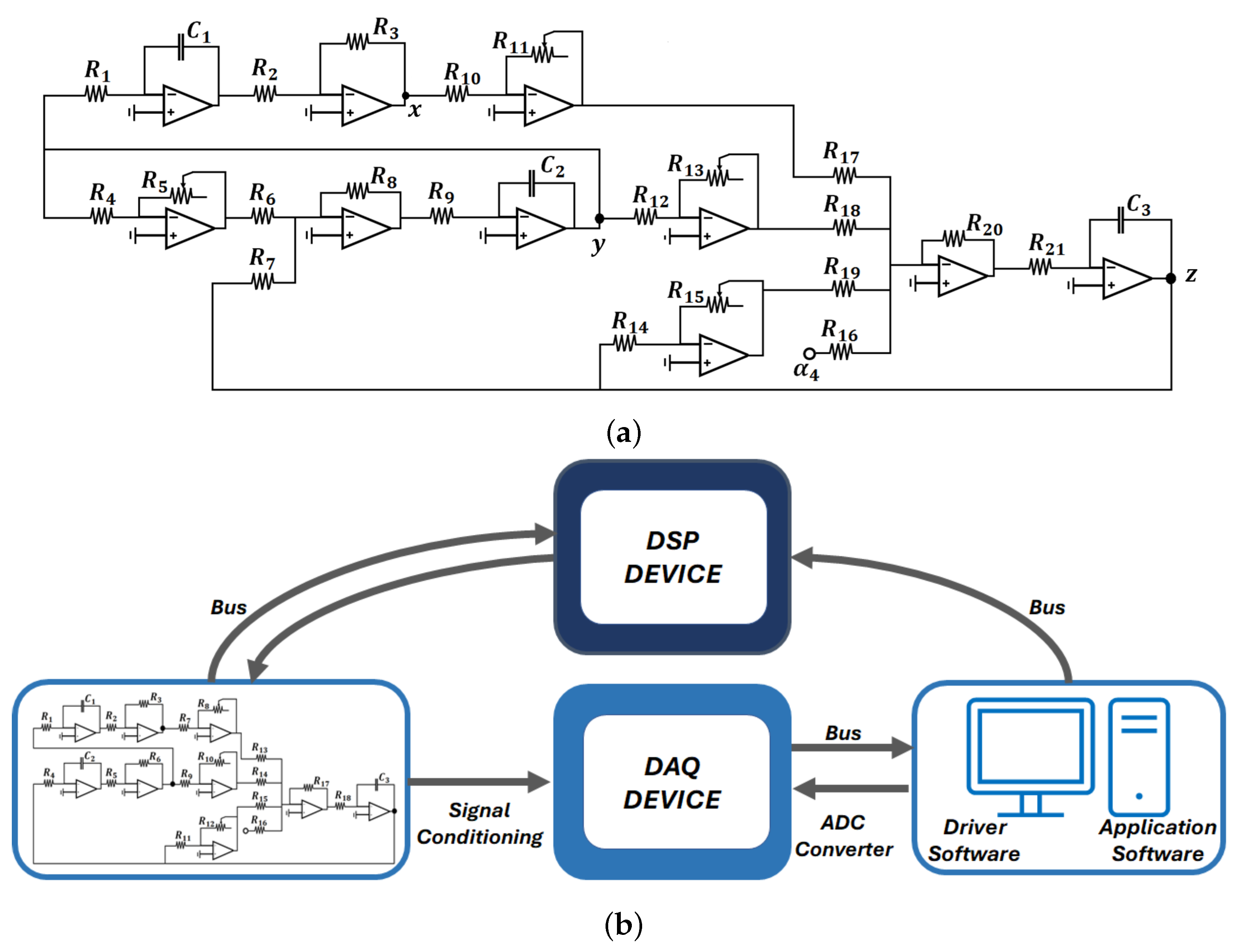
2.2. Electronic Implementation

In recent decades, the study of natural phenomena has intensified through the use of models based on both analog and discrete devices, such as the study of chemical reactions [43], biological systems [44], and neuronal models [45]. The implementation of systems by op-amps is able to remove the limitations of computational calculation and thus produce an analog system that represents the mathematical model under study.

The electronic implementation of the system described by Equations (3) and (4) is based on the properties of the analog computation achieved by using operational amplifiers (op-amps) [46]. The electronic diagram shown in Figure 1a corresponds to the implementation of the linear system, while the nonlinear function ${\alpha }_4$ is embedded in a DSP (Digital Signal Processor) [47]. The electronic circuit solves the system of differential equations, the state variable x is fed into the DSP so that it performs the commutations considering the first state of the system and returns the function ${\alpha }_4$ through one of its DA (Digital-Analogic) channels, which is fed back into the third state variable of the electronic circuit and completes the system.

Since we work with time series generated by the electronic circuit, we perform the storage of the time series through a DAQ (Data Acquisition) system [48]. Given the nonlinear nature of the oscillator, changes in the initial conditions of the analog implementation are accounted via a relay circuit. The initial conditions are randomly changed in the three state variables, enabling and disabling the polarization of the electronic circuit, taking into account the charging and discharging times of the used capacitors. Figure 1b outlines the experimental implementation, which includes the electronic circuit, the DSP to generate the switching function, the DAQ system for data acquisition, and the computer that controls the DAQ, the DSP, and the change in initial conditions.

Considering that the system of the deterministic Brownian-like motion generator has four parameters ($\gamma ,{\alpha }_1,{\alpha }_2,{\alpha }_3$), the possible combinations for the system that can be described by UDS I are almost infinite. Therefore, setting $\gamma =0.1$, a parameter related to a real fluid and particle dimensions, values close to those published in [24] are taken; ${\alpha }_1=1.5,{\alpha }_2=1.3,{\alpha }_3=0.1$. As described in the article proposing the studied system, the constant $C_2=0.6$ determines the size of the segmentations between the switching surfaces, while $C_1={\alpha }_1{C}_2$. The electronic components from Figure 1a are described in

Table 1. Values used in the electronic implementation of the deterministic Brownian-like motion generator.

$\mathbf{Component}$	$\mathbf{Value}$	$\mathbf{Component}$	$\mathbf{Value}$
$R_1,R_9,R_{21}$	1 M$\mathrm{\Omega }$	$R_4$	100 K$\mathrm{\Omega }$
$R_{10},R_{12},R_{14}$	10 K$\mathrm{\Omega }$	$R_5,R_{11}$	[1–100] K$\mathrm{\Omega }$
$R_2,R_3,R_6,R_7$	1 K$\mathrm{\Omega }$	$C_1,C_2,C_3$	100 pF
$R_5,R_{11},R_{13},R_{15}$	[1–100] K$\mathrm{\Omega }$	$R_8,R_{16},R_{17},R_{18},R_{19},R_{20}$	1 K$\mathrm{\Omega }$

, while the ratios describing the system parameters are as follows:

$$\begin{array}{c}{\displaystyle \frac{R_{11}}{R_{10}}}={\alpha }_1;{\displaystyle \frac{R_{13}}{R_{12}}}={\alpha }_2;{\displaystyle \frac{R_{15}}{R_{14}}}={\alpha }_3;{\displaystyle \frac{R_5}{R_4}}=\gamma .\hfill \end{array}$$

(6)

2.3. Statistical Metrics

The metrics used to characterize the dynamics of the electronic circuit are described below. It is important to emphasize that a Brownian-like motion is desired in the system variable x, which is associated with the position of the particle.

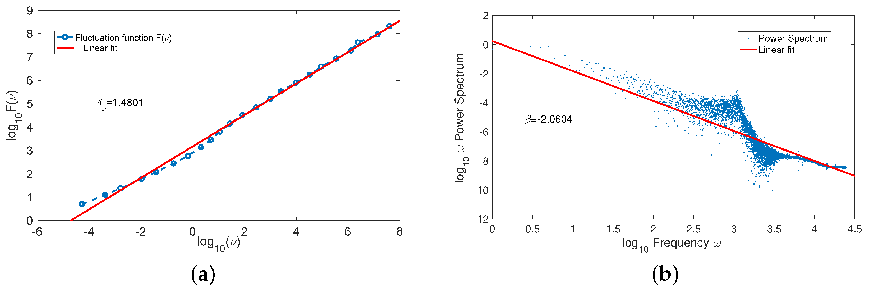
2.3.1. Detrendred Fluctuation Analysis

Detrended Fluctuation Analysis (DFA) is a scaling method used to estimate long-range temporal correlations in the form of a power law. The main advantage of DFA over many other methods is that it allows the detection of long-range correlations of the signal embedded in apparently non-stationary time series, and also avoids the spurious detection of apparent long-range correlations that are an artifact of non-stationarity. The fluctuation function $F(v;s)$ obeys the power law scaling relation described in Equation (7). The method was first proposed in 1994 by C.K. Peng [49], and better described in [24,25], who used this type of analysis to identify trends in DNA strands without knowing their shape or origin.

$$\begin{array}{c}F(v;s)\sim s^{{\delta }_v},\hfill \end{array}$$

(7)

where s are the segments from the time series with length $\nu$. The typical classes of correlations associated with the exponent ${\delta }_v$ are the following:

• When ${\delta }_v=0.5$, the time series is said to be uncorrelated, white noise.
• When $0<{\delta }_v<0.5$, the time series is anti-correlated.
• If $0.5<{\delta }_v<1$, there are extensive positive correlations in the series under study.
• If ${\delta }_v=1$, the signal corresponds to a $\raisebox{1ex}{$1$}\!\left/ \!\raisebox{-1ex}{$f$}\right.$-type process, pink noise.
• If ${\delta }_v\sim 1.5$, the signal shows a Brownian-like behavior, brown noise.

2.3.2. Power Law in the Power Spectrum

Another important feature of Brownian motion is its Lorentzian shape of the power spectrum with a $-2$ power law of the high-frequency slope, which obeys the scaling relation

$$\begin{array}{c}I\left(\omega \right)\sim {\omega }^{\beta },\hfill \end{array}$$

(8)

where $I\left(\omega \right)$ is the spectral intensity at frequency $\omega$. According to the observations on a colloidal particle in a liquid [50], Brownian motion has an exponent of $\beta \sim -2$.

After calculating the Fourier transform of the time series, it is plotted on a log-log scale to later calculate its slope using least squares. The slope value obtained is the one associated with the power law.

2.3.3. Mean Square Displacement

Let there be a particle with Brownian behavior, where any change in its position can be either forward or backward, which cannot be predicted and has the same probability of occurrence. If you want to know the distance traveled by the particle and take a known point as the starting point, it would be sufficient to add the distances traveled at each instant. However, since a forward motion increases the distance and a backward motion decreases it, and since both events have the same probability of occurrence, the distance obtained at the end would be zero. For this reason, Einstein defined the distance traveled by a particle with random behavior as the square of the distance traveled at each instant, generating a sum of positive elements that allow quantifying the distance traveled by the particle under study [7,51]. The formula describing this measure, the Mean Square Displacement (MSD), can be represented as in Equation (9), where $x\left(t\right)$ is each of the directional changes of the particle and $x\left(0\right)$ is the starting point taken as reference. Brownian motion is characterized by the fact that the Mean Square Displacement grows linearly with time.

$$\begin{array}{c}\mathrm{MSD}=\overline{∆x^2}=〈{(x\left(t\right)-x\left(0\right))}^2〉.\hfill \end{array}$$

(9)

2.3.4. Normal Probability Distribution

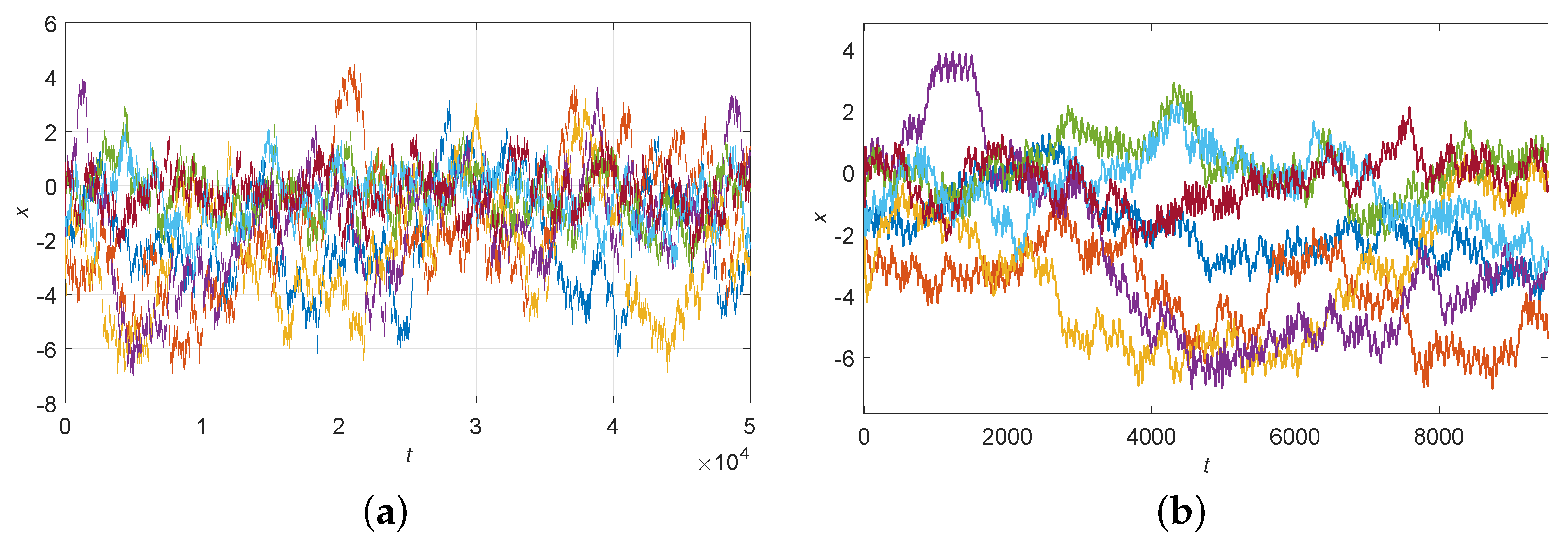
The normal distribution was first recognized by Abraham Moivre. Later, Carl Gauss deepened his study and established the equation of the normal curve, also known as the Gaussian curve [52,53]. The distribution of a normal variable is determined by two parameters, its mean (usually represented as $\mu$), and the standard deviation ($\sigma$). This gives the density of a normal curve as Equation (10), which can be used to generate the characteristics of the Gaussian bell curve. It is known that Brownian motion is characterized by Gaussian probability distributions of particle position.

$$\begin{array}{c}f\left(x\right)={\displaystyle \frac{1}{\sqrt{2\pi \sigma }}}e\left(-{\displaystyle \frac{{(x-\mu )}^2}{2{\sigma }^2}}\right);-\infty <x<+\infty \hfill \end{array}.$$

(10)

3. Results

The results obtained by applying the four statistical metrics we use to characterize deterministic Brownian-like motion are shown below. The time series shown in Figure 2 were obtained by randomly changing the initial conditions for the values $\gamma =0.1,$ ${\alpha }_1=1.5,{\alpha }_2=1.3,{\alpha }_3=0.1,C_1=0.9,C_2=0.6$ used in the electronic oscillator described by Equation (3) and shown in Figure 1a. As can be seen, the behavior is different for each initial condition, as expected for Brownian motion.

Let us first consider the DFA analysis applied to the time series, which gives us values in the range of $1.38<{\delta }_{\nu }<1.6$, expected values for stochastic Brownian behavior. Figure 3a shows the fluctuation function resulting from the analysis of the purple time series shown in Figure 2. It has an exponent of ${\delta }_{\nu }=1.4801$, which is consistent with what is expected for a Brownian-like behavior. A similar result can be obtained for a different initial condition with the same parameters, which confirms the DFA evaluation.

Once the time series is validated with DFA, its power spectrum is calculated by the Fourier transform and its power law is determined. Figure 3b shows the power spectrum of the same time series to which DFA was applied, yielding a power law $\beta =-2.012$. As described in Section 2, Brownian-like behaviors are characterized by power laws in the frequency spectrum close to $-2$.

After validating the dynamics of the system using DFA and the power law in the frequency spectrum, we analyze whether the probability distribution of the time series resembles a normal distribution. Figure 4a shows the histogram of the analyzed time series and the approximation to a normal distribution with mean and standard deviation that the time series has. This result is confirmed by a Normal-plot, Figure 4b. This type of graph is used to analyze whether the analyzed data correspond to what is expected from a normal distribution. The results show that the analyzed time series are normally distributed with certain tolerances.

Finally, the behavior of the mean square displacement of the time series is analyzed. Figure 5a shows the behavior of the MSD of a Brownian time series according to Einstein’s findings. Similarly, and using Equation (9) to calculate the MSD, Figure 5b shows the behavior of $\overline{∆x^2}$ for the same purple time series depicted in Figure 2, consistent with a linear increase over time.

4. Discussion

The results described in the previous section are restricted to the range of values where $C_1={\alpha }_1{C}_2$. However, when the parameter $C_1$ is considered variable, the system shows multiscroll dynamics with a variable number of scrolls, similar to that published in [46,54]. Considering this, the oscillator described by Equation (3) is able to exhibit many more behaviors than deterministic Brownian-like motion, such as white noise, pink noise, periodic behavior, and even coexistence of attractors. It is worth noting that both the scroll generation with the highest number and the regions where the system exhibits Brownian-like motion are described by $C_1={\alpha }_1{C}_2$.

Remark 1.

It is worth noting that the metrics used were exclusive, i.e., they were applied in the order described below and the combination of values was excluded if the tests were not passed:

1. 

DFA;

2. 

Power law in the frequency spectrum;

3. 

Normal probability distribution;

4. 

Mean Square Displacement.

As mentioned in the previous sections, in this work, the behavior of the electronic circuit shown in Figure 1 was analyzed for 126 combinations of values of the parameters ${\alpha }_i$. These combinations of values are described in

Table A1. Explored values in the electronic implementation of the deterministic Brownian-like motion generator.

${\mathit{\alpha }}_1$	${\mathit{\alpha }}_2$	${\mathit{\alpha }}_3$	$-{\mathit{\sigma }}_1$	${\mathit{\sigma }}_2$	${\mathit{\rho }}_2$	${\displaystyle \sum _{\mathit{i}=1}^3{\mathit{\lambda }}_{\mathit{i}}}$	${\mathit{\alpha }}_1$	${\mathit{\alpha }}_2$	${\mathit{\alpha }}_3$	$-{\mathit{\sigma }}_1$	${\mathit{\sigma }}_2$	${\mathit{\rho }}_2$	${\displaystyle \sum _{\mathit{i}=1}^3{\mathit{\lambda }}_{\mathit{i}}}$
$0.7$	$0.7$	$0.1$	$0.67$	$0.23$	$0.98i$	$-0.2$	$0.9$	$0.7$	$0.1$	$0.47$	$0.03$	$1.21i$	$-0.4$
$0.7$	$0.7$	$0.3$	$0.72$	$0.16$	$0.96i$	$-0.4$	$0.9$	$0.7$	$0.3$	$0.82$	$0.21$	$1.01i$	$-0.4$
$0.7$	$0.7$	$0.5$	$0.78$	$0.09$	$0.94i$	$-0.6$	$0.9$	$0.7$	$0.5$	$0.89$	$0.14$	$0.99i$	$-0.6$
$0.7$	$0.7$	$0.6$	$0.81$	$0.05$	$0.92i$	$-0.7$	$0.9$	$0.7$	$0.7$	$0.96$	$0.08$	$0.96i$	$-0.8$
$0.7$	$0.7$	$0.7$	$0.85$	$0.02$	$0.90i$	$-0.8$	$0.9$	$0.7$	$0.8$	$1.0$	$0.1$	$0.94i$	$-0.8$
$0.7$	$0.9$	$0.1$	$0.60$	$0.20$	$1.05i$	$-0.2$	$0.9$	$0.7$	$0.9$	$1.05$	$0.02$	$0.92i$	$-1$
$0.7$	$0.9$	$0.2$	$0.62$	$0.16$	$1.04i$	$-0.3$	$0.9$	$0.9$	$0.1$	$0.70$	$0.25$	$1.09i$	$-0.2$
$0.7$	$0.9$	$0.4$	$0.66$	$0.08$	$1.02i$	$-0.5$	$0.9$	$0.9$	$0.3$	$0.75$	$0.17$	$1.07i$	$-0.4$
$0.7$	$0.9$	$0.5$	$0.69$	$0.04$	$1.00i$	$-0.6$	$0.9$	$0.9$	$0.5$	$0.80$	$0.10$	$1.05i$	$-0.6$
$0.7$	$1.0$	$0.1$	$0.57$	$0.18$	$1.09i$	$-0.2$	$0.9$	$0.9$	$0.7$	$0.87$	$0.03$	$1.01i$	$-0.8$
$0.7$	$1.0$	$0.3$	$0.60$	$0.10$	$1.06i$	$-0.4$	$0.9$	$1.1$	$0.1$	$0.64$	$0.22$	$1.16i$	$-0.2$
$0.7$	$1.0$	$0.5$	$0.64$	$0.02$	$1.03i$	$-0.6$	$0.9$	$1.1$	$0.3$	$0.68$	$0.14$	$1.14i$	$-0.4$
$0.7$	$1.1$	$0.2$	$0.55$	$0.12$	$1.11i$	$-0.3$	$0.9$	$1.1$	$0.5$	$0.72$	$0.06$	$1.11i$	$-0.6$
$0.7$	$1.1$	$0.3$	$0.57$	$0.08$	$1.10i$	$-0.4$	$0.9$	$1.3$	$0.1$	$0.58$	$0.19$	$1.22i$	$-0.2$
$0.7$	$1.1$	$0.5$	$0.60$	$.003$	$1.07i$	$-0.6$	$0.9$	$1.3$	$0.3$	$0.61$	$0.10$	$1.20i$	$-0.4$
$0.7$	$1.2$	$0.1$	$0.51$	$0.15$	$1.15i$	$-0.2$	$0.9$	$1.3$	$0.5$	$0.65$	$0.02$	$1.17i$	$-0.6$
$0.7$	$1.2$	$0.2$	$0.52$	$0.11$	$1.15i$	$-0.3$	$0.9$	$1.5$	$0.1$	$0.53$	$0.16$	$1.28i$	$-0.2$
$0.7$	$1.2$	$0.4$	$0.55$	$0.02$	$1.12i$	$-0.5$	$0.9$	$1.5$	$0.2$	$0.54$	$0.12$	$1.27i$	$-0.3$
$0.7$	$1.3$	$0.1$	$0.48$	$0.14$	$1.19i$	$-0.2$	$0.9$	$1.5$	$0.3$	$0.55$	$0.07$	$1.26i$	$-0.4$
$0.7$	$1.3$	$0.2$	$0.49$	$0.09$	$1.18i$	$-0.3$	$0.9$	$1.5$	$0.4$	$0.56$	$0.03$	$1.25i$	$-0.5$
$0.7$	$1.3$	$0.4$	$0.51$	$.009$	$1.16i$	$-0.5$	$0.9$	$1.7$	$0.1$	$0.48$	$0.14$	$1.35i$	$-0.2$
$0.7$	$1.4$	$0.1$	$0.51$	$.009$	$1.16i$	$-0.5$	$0.9$	$1.7$	$0.2$	$0.49$	$0.09$	$1.34i$	$-0.3$
$0.7$	$1.4$	$0.3$	$0.47$	$0.03$	$1.21i$	$-0.4$	$0.9$	$1.7$	$0.3$	$0.50$	$0.05$	$1.33i$	$-0.4$
$0.9$	$1.7$	$0.4$	$0.51$	$.007$	$1.32i$	$-0.5$	$1.1$	$1.7$	$0.3$	$0.59$	$0.09$	$1.35i$	$-0.4$
$1.1$	$0.7$	$0.2$	$0.88$	$0.29$	$1.07i$	$-0.3$	$1.1$	$1.7$	$0.5$	$0.62$	$0.01$	$1.32i$	$-0.6$
$1.1$	$0.7$	$0.4$	$0.94$	$0.22$	$1.05i$	$-0.5$	$1.3$	$0.7$	$0.1$	$0.93$	$0.36$	$1.12i$	$-0.2$
$1.1$	$0.7$	$0.6$	$1.01$	$0.15$	$1.08i$	$-0.7$	$1.3$	$0.7$	$0.5$	$1.05$	$0.22$	$1.08i$	$-0.6$
$1.1$	$0.7$	$0.8$	$1.1$	$0.1$	$0.99i$	$-0.9$	$1.3$	$0.7$	$0.7$	$1.13$	$0.16$	$1.05i$	$-0.8$
$1.1$	$0.7$	$1.0$	$1.19$	$0.04$	$0.95i$	$-1.1$	$1.3$	$0.7$	$1.0$	$1.27$	$0.08$	$1.00i$	$-1.1$
$1.1$	$0.9$	$0.2$	$0.81$	$0.25$	$1.13i$	$-0.3$	$1.3$	$0.7$	$1.3$	$1.44$	$0.02$	$0.94i$	$-1.4$
$1.1$	$0.9$	$0.4$	$0.87$	$0.18$	$1.10i$	$-0.5$	$1.3$	$0.9$	$0.3$	$0.92$	$0.26$	$1.15i$	$-0.4$
$1.1$	$0.9$	$0.6$	$0.93$	$0.11$	$1.07i$	$-0.7$	$1.3$	$0.9$	$0.5$	$0.98$	$0.19$	$1.13i$	$-0.6$
$1.1$	$0.9$	$0.8$	$1.0$	$0.05$	$1.04i$	$-0.9$	$1.3$	$0.9$	$0.7$	$1.05$	$0.12$	$1.1i$	$-0.8$
$1.1$	$0.9$	$1.0$	$1.1$	$0.0$	$1.0i$	$-1.1$	$1.3$	$0.9$	$0.9$	$1.13$	$0.06$	$1.06i$	$-1.0$
$1.1$	$1.1$	$0.1$	$0.73$	$0.26$	$1.19i$	$-0.2$	$1.3$	$1.1$	$0.7$	$0.97$	$0.08$	$1.15i$	$-0.8$
$1.1$	$1.1$	$0.3$	$0.77$	$0.18$	$1.17i$	$-0.4$	$1.3$	$1.1$	$0.9$	$1.04$	$0.02$	$1.11i$	$-1.0$
$1.1$	$1.1$	$0.5$	$0.82$	$0.11$	$1.14i$	$-0.6$	$1.3$	$1.3$	$0.1$	$0.75$	$0.27$	$1.28i$	$-0.2$
$1.1$	$1.1$	$0.7$	$0.88$	$0.04$	$1.11i$	$-0.8$	$1.3$	$1.3$	$0.3$	$0.79$	$0.19$	$1.26i$	$-0.4$
$1.1$	$1.3$	$0.1$	$0.67$	$0.23$	$1.25i$	$-0.2$	$1.3$	$1.3$	$0.5$	$0.83$	$0.11$	$1.23i$	$-0.6$
$1.1$	$1.3$	$0.3$	$0.7$	$0.15$	$1.23i$	$-0.4$	$1.3$	$1.3$	$0.7$	$0.89$	$0.04$	$1.20i$	$-0.8$
$1.1$	$1.3$	$0.5$	$0.75$	$0.07$	$1.2i$	$-0.6$	$1.3$	$1.5$	$0.1$	$0.69$	$0.24$	$1.34i$	$-0.2$
$1.1$	$1.3$	$0.7$	$0.80$	$.001$	$1.17i$	$-0.8$	$1.3$	$1.5$	$0.3$	$0.73$	$0.16$	$1.32i$	$-0.4$
$1.1$	$1.5$	$0.1$	$0.62$	$0.21$	$1.31i$	$-0.2$	$1.3$	$1.5$	$0.5$	$0.77$	$0.08$	$1.29i$	$-0.6$
$1.1$	$1.5$	$0.3$	$0.64$	$0.12$	$1.29i$	$-0.4$	$1.3$	$1.5$	$0.7$	$0.81$	$0.009$	$1.25i$	$-0.8$
$1.1$	$1.5$	$0.5$	$0.68$	$0.04$	$1.26i$	$-0.6$	$1.3$	$1.7$	$0.1$	$0.64$	$0.22$	$1.39i$	$-0.2$
$1.1$	$1.7$	$0.1$	$0.57$	$0.18$	$1.37i$	$-0.2$	$1.3$	$1.7$	$0.3$	$0.67$	$0.13$	$1.37i$	$-0.4$
$1.3$	$1.7$	$0.5$	$0.71$	$0.05$	$1.35i$	$-0.6$	$1.5$	$1.1$	$0.3$	$0.92$	$0.26$	$1.24i$	$-0.4$
$1.5$	$0.7$	$0.1$	$0.99$	$0.39$	$1.16i$	$-0.2$	$1.5$	$1.1$	$0.5$	$0.98$	$0.19$	$1.22i$	$-0.6$
$1.5$	$0.7$	$0.3$	$1.05$	$0.32$	$1.14i$	$-0.4$	$1.5$	$1.1$	$0.7$	$1.04$	$0.12$	$1.18i$	$-0.8$
$1.5$	$0.7$	$0.5$	$1.12$	$0.26$	$1.12i$	$-0.6$	$1.5$	$1.1$	$0.9$	$1.12$	$0.06$	$1.15i$	$-1.0$
$1.5$	$0.7$	$0.7$	$1.2$	$0.2$	$1.1i$	$-0.8$	$1.5$	$1.1$	$1.1$	$1.21$	$.008$	$1.10i$	$-1.2$
$1.5$	$0.7$	$0.9$	$1.28$	$0.14$	$1.06i$	$-1.0$	$1.5$	$1.3$	$0.1$	$0.82$	$0.31$	$1.31i$	$-0.2$
$1.5$	$0.7$	$1.1$	$1.39$	$0.09$	$1.03i$	$-1.2$	$1.5$	$1.3$	$0.3$	$0.86$	$0.23$	$1.29i$	$-0.4$
$1.5$	$0.7$	$1.3$	$1.5$	$0.05$	$0.99i$	$-1.4$	$1.5$	$1.3$	$0.5$	$0.91$	$0.15$	$1.27i$	$-0.6$
$1.5$	$0.7$	$1.5$	$1.63$	$0.01$	$0.95i$	$-1.6$	$1.5$	$1.3$	$0.7$	$0.97$	$0.08$	$1.23i$	$-0.8$
$1.5$	$0.9$	$0.1$	$0.93$	$0.36$	$1.21i$	$-0.2$	$1.5$	$1.5$	$0.1$	$0.76$	$0.28$	$1.36i$	$-0.2$
$1.5$	$0.9$	$0.3$	$0.99$	$0.29$	$1.19i$	$-0.4$	$1.5$	$1.5$	$0.3$	$0.80$	$0.20$	$1.34i$	$-0.4$
$1.5$	$0.9$	$0.5$	$1.05$	$0.22$	$1.17i$	$-0.6$	$1.5$	$1.5$	$0.5$	$0.85$	$0.12$	$1.32i$	$-0.6$
$1.5$	$0.9$	$0.7$	$1.12$	$0.16$	$1.14i$	$-0.8$	$1.5$	$1.5$	$0.7$	$0.90$	$0.05$	$1.28i$	$-0.8$
$1.5$	$0.9$	$0.9$	$1.2$	$0.1$	$1.1i$	$-1.0$	$1.5$	$1.7$	$0.1$	$0.71$	$0.25$	$1.42i$	$-0.2$
$1.5$	$0.9$	$1.1$	$1.3$	$0.05$	$1.07i$	$-1.2$	$1.5$	$1.7$	$0.3$	$0.75$	$0.17$	$1.40i$	$-0.4$
$1.5$	$0.9$	$1.3$	$1.41$	$.009$	$1.02i$	$-1.4$	$1.5$	$1.7$	$0.5$	$0.78$	$0.09$	$1.37i$	$-0.6$
$1.5$	$1.1$	$0.1$	$0.87$	$0.33$	$1.26i$	$-0.2$	$1.5$	$1.7$	$0.7$	$0.83$	$0.01$	$1.34i$	$-0.8$

in Appendix A, and lie within the ranges described by (11). Examination and characterization of all of these value combinations, where the value $\gamma$ was held constant, have shown that the combinations shown in

Table 2. Combinations of examined values that have Brownian-like motion based on the analysis performed. For each combination of values, its eigenvalues and the sum of these values are shown to confirm the dissipative conditions of the system. Consider the eigenvalues ${\lambda }_i$, the real component ${\sigma }_i$, and the corresponding imaginary component ${\rho }_i$.

$\mathbf{Comb}.$	${\mathit{\alpha }}_1$	${\mathit{\alpha }}_2$	${\mathit{\alpha }}_3$	$-{\mathit{\sigma }}_1$	${\mathit{\sigma }}_2$	${\mathit{\rho }}_2$	$\mathbf{Comb}.$	${\mathit{\alpha }}_1$	${\mathit{\alpha }}_2$	${\mathit{\alpha }}_3$	$-{\mathit{\sigma }}_1$	${\mathit{\sigma }}_2$	${\mathit{\rho }}_2$
$C_1$	$0.7$	$0.7$	$0.1$	$0.67$	$0.23$	$0.98i$	$C_7$	$1.5$	$0.9$	$0.3$	$0.99$	$0.29$	$1.19i$
$C_2$	$0.9$	$0.7$	$0.5$	$0.89$	$0.14$	$0.99i$	$C_8$	$1.5$	$1.1$	$0.1$	$0.87$	$0.33$	$1.26i$
$C_3$	$1.1$	$1.1$	$0.7$	$0.88$	$0.04$	$1.11i$	$C_9$	$1.5$	$1.3$	$0.1$	$0.82$	$0.31$	$1.31i$
$C_4$	$1.3$	$0.7$	$0.7$	$1.13$	$0.16$	$1.05i$	$C_{10}$	$1.5$	$1.3$	$0.3$	$0.86$	$0.26$	$1.29i$
$C_5$	$1.5$	$0.7$	$0.7$	$1.20$	$0.20$	$1.10i$	$C_{11}$	$1.5$	$1.7$	$0.3$	$0.75$	$0.17$	$1.40i$
$C_6$	$1.5$	$0.7$	$1.3$	$1.5$	$0.05$	$0.99i$	$C_{12}$	$1.5$	$1.7$	$0.7$	$0.83$	$0.01$	$1.34i$

satisfy the metrics established for Brownian behavior.

$$\begin{array}{c}{\alpha }_1=[0.7,1.5],\hfill \\ {\alpha }_2=[0.7,1.7],\hfill \\ {\alpha }_3=[0.1,1.5].\hfill \end{array}$$

(11)

Remark 2.

Note that the random choice of ${\alpha }_i$ values within the ranges described by (11) does not guarantee the oscillation of the electronic circuit. This must always satisfy Proposition 1.

5. Conclusions

In the present work, the implementation and characterization of an oscillator defined by a system of deterministic differential equations was carried out. The dynamics of the oscillator has been studied in search of random-like dynamics similar to that of a Brownian behavior by examining the responses based on four studies whose values are defined for the desired dynamics: (i) the application of Detrended Fluctuation Analysis, (ii) the search for scaling laws in the power spectrum, (iii) the existence of Normal type components in the response of the system, and (iv) the behavior of the mean square displacement.

The results obtained with the circuit implementation show satisfactory agreement with the numerical model [24]. By characterizing the global dynamics of the system, combinations of values for the parameters ${\alpha }_i$ were found for which the dynamics of the oscillator corresponds to what would be expected for a system with Brownian dynamics. This result not only confirms what has been proposed theoretically [24,25], but also extends the possible combinations of values at which the system can exhibit Brownian-like motion.

Remark 3.

It is worth emphasizing that the main contribution of this work is summarized in the following points:

• It is the first electronic implementation that generates Brownian motion in a deterministic way, based on a set of differential equations based on the Langevin equation, i.e., the model takes into account the information of the particles and the surrounding medium.
• The elimination of the stochastic component enables the reproducibility of the results.
• The validation of Brownian-like motion in electronic circuits opens the possibility of using this circuit as seed for applications in the field of medicine, ecology, to name a few.

So far, the idea of generating deterministic Brownian-like motions has been explored only theoretically, without investigating its physical implementation. Our work fills this gap by electronically confirming the generation of said behavior by eliminating the stochastic component, thus enabling reproducibility of the results. Once we have implemented an electronic circuit capable of generating Brownian-like motion in a deterministic manner, it can be used as a noise source due to the properties that define Brownian motion and thus has potential applications in fields such as medicine, economics, genetics, and communications, to name a few. Comparing the results based on classical Brownian motion described by the Langevin equation with those described by the electronic circuit is part of the research group’s future work.

References

1. Osborne, M.F. Brownian motion in the stock market. Oper. Res. 1959, 7, 145–173. [Google Scholar] [CrossRef]
2. Ermogenous, A. Brownian Motion and Its Applications in the Stock Market; University of Dayton: Dayton, OH, USA, 2006. [Google Scholar]
3. Lima, M.A.F.; Fernández Ramírez, L.M.; Carvalho, P.; Batista, J.G.; Freitas, D.M. A comparison between deep learning and support vector regression techniques applied to solar forecast in Spain. J. Sol. Energy Eng. 2022, 144, 010802. [Google Scholar] [CrossRef]
4. Xiao, D.; Chen, H.; Wei, C.; Bai, X. Statistical Measure for Risk-Seeking Stochastic Wind Power Offering Strategies in Electricity Markets. J. Mod. Power Syst. Clean Energy 2021. to be published. [Google Scholar] [CrossRef]
5. Toral, R. Últimos Avances en el Movimiento Browniano: Orden a Partir del Desorden, Cien años de Herencia Einsteiniana; Instituto Mediterráneo de Estudios Avanzados (IMEDEA); CSIC-Universitat de les Illes Balears: Palma de Mallorca, Spain, 2008. [Google Scholar]
6. Brown, R. A Brief Account of Microscopical Observations Made... on the Particles Contained in the Pollen of Plants, and on the General Existence of Active Molecules in Organic and Inorganic Bodies; Cambridge University Press: Cambridge, UK, 1828. [Google Scholar]
7. Einstein, A. Investigations on the Theory of the Brownian Movement; Courier Corporation: Chelmsford, MA, USA, 1956. [Google Scholar]
8. Langevin, P. Sur la théorie du mouvement brownien. CR Acad. Sci. Paris 1908, 146, 530. [Google Scholar]
9. Perrin, J. Discontinuous Structure of Matter; Nobel Lecture Nobel.Price.org; 1926. Available online: https://www.nobelprize.org/prizes/physics/1926/perrin/lecture/ (accessed on 15 July 2017).
10. Smoluchowski, M. Investigation into a Mathematical Theory of the Kinetics of Coagulation of Colloidal Solutions; Army Biological Labs: Frederick, MD, USA, 1967. [Google Scholar]
11. Fokker, A.D. Over Browns’che Bewegingen in Het Stralingsveld. Ph.D. Thesis, Physics and Mathematics Faculty, University of Leiden, Leiden, The Netherlands, 1913. [Google Scholar]
12. Planck, M. Vorlesungen uber Thermodynamik; De Gruyter: Berlin, Germany, 1927. [Google Scholar]
13. Ornstein, L. On the Brownian motion. In Proceedings, 21 I; KNAW: Amsterdam, The Netherlands, 1919; Volume 21, pp. 96–108. [Google Scholar]
14. Burger, H. Over de theorie der Brown’sche beweging. Versl. Kon. Ak 1917, 25, 1482. [Google Scholar]
15. Ren, Y.; Yin, W.; Sakthivel, R. Stabilization of stochastic differential equations driven by G-Brownian motion with feedback control based on discrete-time state observation. Automatica 2018, 95, 146–151. [Google Scholar] [CrossRef]
16. Yang, H.; Ren, Y.; Lu, W. Stabilisation of stochastic differential equations driven by G-Brownian motion via aperiodically intermittent control. Int. J. Control 2020, 93, 565–574. [Google Scholar] [CrossRef]
17. Duan, P. Stabilization of stochastic differential equations driven by G-Brownian motion with aperiodically intermittent control. Mathematics 2021, 9, 988. [Google Scholar] [CrossRef]
18. Van Hove, L. Quantum-mechanical perturbations giving rise to a statistical transport equation. Physica 1954, 21, 517–540. [Google Scholar] [CrossRef]
19. Zwanzig, R. Lectures in Theoretical Physics; Brittin, W.E., Downs, B.W., Downs, J., Eds.; Interscience: New York, NY, USA, 1961; Volume 3, p. 106. [Google Scholar]
20. Grigolini, P.; Rocco, A.; West, B.J. Fractional calculus as a macroscopic manifestation of randomness. Phys. Rev. E 1999, 59, 2603. [Google Scholar] [CrossRef]
21. West, B.J.; Grigolini, P.; Metzler, R.; Nonnenmacher, T.F. Fractional diffusion and Lévy stable processes. Phys. Rev. E 1997, 55, 99. [Google Scholar] [CrossRef]
22. Dettmann, C.P.; Cohen, E.; Van Beijeren, H. Statistical mechanics: Microscopic chaos from brownian motion? Nature 1999, 401, 875. [Google Scholar] [CrossRef] [Green Version]
23. Trefán, G.; Grigolini, P.; West, B.J. Deterministic brownian motion. Phys. Rev. A 1992, 45, 1249. [Google Scholar] [CrossRef] [PubMed]
24. Huerta-Cuellar, G.; Jimenez-Lopez, E.; Campos-Cantón, E.; Pisarchik, A. An approach to generate deterministic Brownian motion. Commun. Nonlinear Sci. Numer. Simul. 2014, 19, 2740–2746. [Google Scholar] [CrossRef]
25. Gilardi-Velázquez, H.E.; Campos-Cantón, E. Nonclassical point of view of the Brownian motion generation via fractional deterministic model. Int. J. Mod. Phys. C 2018, 29, 1850020. [Google Scholar] [CrossRef]
26. Prada, D.; Herrera-Jaramillo, Y.; Ortega, J.; Gómez, J. Fractional Brownian motion and Hurst coefficient in drinking water turbidity analysis. J. Phys. Conf. Ser. 2020, 1645, 012004. [Google Scholar] [CrossRef]
27. Herrera, Y.; Prada, D.; Ortega, J.; Sierra, A.; Acevedo, A. Physical applications: Fractional Brownian movement applied to the particle dispersion. J. Phys. Conf. Ser. 2020, 1702, 012004. [Google Scholar] [CrossRef]
28. Prada, D.; Acevedo, A.; Fernandez, H.; Prada, S.; Gómez, J. Physical applications: Analysis of Colombian coffee prices using fractional Brownian motion. J. Phys. Conf. Ser. 2020, 1645, 012002. [Google Scholar] [CrossRef]
29. Rahman, Z.A.S.; Jasim, B.H.; Al-Yasir, Y.I.; Abd-Alhameed, R.A.; Alhasnawi, B.N. A new no equilibrium fractional order chaotic system, dynamical investigation, synchronization, and its digital implementation. Inventions 2021, 6, 49. [Google Scholar] [CrossRef]
30. Balcerek, M.; Burnecki, K. Testing of multifractional Brownian motion. Entropy 2020, 22, 1403. [Google Scholar] [CrossRef]
31. Yang, Y.; Zhu, H.; Lai, D. Estimating Conditional Power for Sequential Monitoring of Covariate Adaptive Randomized Designs: The Fractional Brownian Motion Approach. Fractal Fract. 2021, 5, 114. [Google Scholar] [CrossRef]
32. Martín-Pasquín, F.J.; Pisarchik, A.N. Brownian Behavior in Coupled Chaotic Oscillators. Mathematics 2021, 9, 2503. [Google Scholar] [CrossRef]
33. Armijo, J. Absorción, distribución y eliminación de los fármacos. In Farmacología Humana; Masson, SA: Barcelona, Spain, 1997; pp. 47–72. [Google Scholar]
34. del Carmen Avendaño-López, M. La paradoja farmacéutica: Anticancerosos basados en la hipoxia celular. Inhibidores PARP. In The Anales de la Real Sociedad Española de Química; Number 4; Real Sociedad Española de Química: Madrid, Spain, 2012; pp. 290–297. [Google Scholar]
35. Dagdug, L.; Berezhkovskii, A.M.; Shvartsman, S.Y.; Weiss, G.H. Equilibration in two chambers connected by a capillary. J. Chem. Phys. 2003, 119, 12473–12478. [Google Scholar] [CrossRef]
36. Gibaldi, M.; Lee, M.; Desai, A. Gibaldi’s Drug Delivery Systems in Pharmaceutical Care; ASHP: Bethesda, MD, USA, 2007. [Google Scholar]
37. Stokes, G.G. On the Effect of the Internal Friction of Fluids on the Motion of Pendulums; Pitt Press: Pittsburgh, PA, USA, 1851; Volume 9. [Google Scholar]
38. Štefan Porubský. Integer Rounding Functions. Available online: https://www.cs.cas.cz/portal/AlgoMath/NumberTheory/ArithmeticFunctions/IntegerRoundingFunctions.htm (accessed on 20 January 2016).
39. Lu, J.; Chen, G.; Yu, X.; Leung, H. Design and analysis of multiscroll chaotic attractors from saturated function series. IEEE Trans. Circuits Syst. I Regul. Pap. 2004, 51, 2476–2490. [Google Scholar] [CrossRef]
40. Gilardi-Velázquez, H.; Ontañón-García, L.; Hurtado-Rodriguez, D.; Campos-Cantón, E. Multistability in Piecewise Linear Systems by Means of the Eigenspectra Variation and the Round Function. arXiv 2016, arXiv:1611.03461. [Google Scholar]
41. Gilardi-Velázquez, H.; Ontañón-García, L.; Hurtado-Rodriguez, D.; Campos-Cantón, E. Multistability in piecewise linear systems versus eigenspectra variation and round function. Int. J. Bifurc. Chaos 2017, 27, 1730031. [Google Scholar] [CrossRef]
42. Anzo-Hernández, A.; Gilardi-Velázquez, H.E.; Campos-Cantón, E. On multistability behavior of unstable dissipative systems. Chaos Interdiscip. J. Nonlinear Sci. 2018, 28, 033613. [Google Scholar] [CrossRef] [PubMed]
43. Holden, A.V.; Fan, Y. From simple to complex oscillatory behaviour via intermittent chaos in the Rose-Hindmarsh model for neuronal activity. Chaos Solitons Fractals 1992, 2, 349–369. [Google Scholar] [CrossRef]
44. Carmona, V.; Freire, E.; Ponce, E.; Torres, F. On simplifying and classifying piecewise-linear systems. IEEE Trans. Circuits Syst. I Fundam. Theory Appl. 2002, 49, 609–620. [Google Scholar] [CrossRef]
45. Chua, L.O.; Yang, L. Cellular neural networks: Applications. IEEE Trans. Circuits Syst. 1988, 35, 1273–1290. [Google Scholar] [CrossRef]
46. Echenausía-Monroy, J.L.; García-López, J.H.; Jaimes-Reátegui, R.; Huerta-Cuéllar, G. Parametric control for multiscroll generation: Electronic implementation and equilibrium analysis. Nonlinear Anal. Hybrid Syst. 2020, 38, 100929. [Google Scholar] [CrossRef]
47. Instruments, N. dSPACE. Available online: https://www.dspace.com/en/pub/home.cfm (accessed on 15 July 2017).
48. Instruments, N. DAQ 6353. Available online: http://www.ni.com/es-mx/support/model.usb-6353.html (accessed on 15 July 2017).
49. Peng, C.K.; Buldyrev, S.V.; Havlin, S.; Simons, M.; Stanley, H.E.; Goldberger, A.L. Mosaic organization of DNA nucleotides. Phys. Rev. E 1994, 49, 1685. [Google Scholar] [CrossRef] [PubMed]
50. Gaspard, P.; Briggs, M.; Francis, M.; Sengers, J.; Gammon, R.; Dorfman, J.R.; Calabrese, R. Experimental evidence for microscopic chaos. Nature 1998, 394, 865–868. [Google Scholar] [CrossRef]
51. Einstein, A. Un the movement of small particles suspended in statiunary liquids required by the molecular-kinetic theory 0f heat. Ann. Phys. 1905, 17, 549–560. [Google Scholar] [CrossRef]
52. Dixon, W.J.; Massey, F.J. Introduction to Statistical Analysis; McGraw-Hill: New York, NY, USA, 1969; Volume 344. [Google Scholar]
53. Triola, M.F. Essentials of Statistics; Pearson/Addison Wesley: Boston, MA, USA, 2005. [Google Scholar]
54. Echenausía-Monroy, J.L.; García-López, J.H.; Jaimes-Reátegui, R.; Huerta-Cuellar, G. Electronic implementation dataset to monoparametric control the number of scrolls generated. Data Brief 2020, 31, 105992. [Google Scholar] [CrossRef]
Figure 1. (a) Circuit diagram of the generator for Brownian-like motion described by Equation (3). (b) Experimental setup for data acquisition from electronic implementation.
Electronics 11 02949 g001
Figure 2. (a) Time series generated by the electronic circuit shown in Figure 1 for parameters γ = 0.1 , α 1 = 1.5 , α 2 = 1.3 , α 3 = 0.1 , C 1 = 0.9 , C 2 = 0.6 . (b) Zoom-in on the time series shown in (a).
Electronics 11 02949 g002
Figure 3. (a) DFA for the time series obtained from the electronic circuit. (b) Power law analysis of the frequency spectrum.
Electronics 11 02949 g003
Figure 4. (a) (Doted line) The probability density resulting from the variable x generated by the electronic circuit is represented by the normalized histogram, compared with the approximation resulting from the evaluation of the time series by the Gaussian function (solid line). (b) Normal plot of the analyzed time series (blue line) against the estimated approximation (red line).
Electronics 11 02949 g004
Figure 5. (a) Mean Square Displacement (MSD) of a Brownian particle. (b) MSD for the time series generated by the electronic circuit.
Electronics 11 02949 g005