Non-Linear Inductor Models Comparison for Switched-Mode Power Supplies Applications

Highlights

• Purpose of the paper: to compare two analytical models of non-linear power inductor to be employed in an SMPS in the same test conditions.
• Methodology: the models are identified by an experimental setup. It exploits the same DC/DC converter board used for simulations. The computation time and accuracy are compared, on the same computer, retrieving the characteristic curve, calculating a current profile and performing a simulation of a boost converter employing the identified models.
• Research limits: (a) the absolute computation time evaluation could be performed by the algorithmic complexity function; in this paper we provided a the relative comparison between the two algorithms; (b) most manufacturers do not give enough information to identify the model valid up to the saturation region; as a consequence, a dedicated measurement system is required.
• Practical implications: the user can choose the model according to a trade-off between computation time and operation outside the rated current interval.
• Originality of the paper: it is the first time that the two models are compared in the same test conditions showing the pros and cons of each.

Abstract

The use of non-linear power inductors, intended as devices exploited up to a current at which the inductance is halved, is of great interest in switched-mode power supplies (SMPSs). Indeed, it allows the use of lighter and cheaper inductors improving the power density. On the other hand, the analysis of SMPSs equipped with non-linear inductors requires appropriate modeling of the inductor reproducing the inductance versus current. This paper compares two main analytical models proposed in the literature: the former is based on a polynomial, and the latter exploits the arctangent function to reproduce the non-linearity of the inductance. Performance is compared by considering the effort of retrieving the model’s parameters, evaluating a current profile by the characteristic equation of the inductor, and exploiting the two models to simulate a switched-mode power supply. Results are given both in terms of computation time and accuracy with reference to experimental values, highlighting the pros and cons of each model.

1. Introduction

In most power electronic circuits, the requirements to limit space and weight are essential. Among the adopted solutions for striving the highest possible power density, there are, for example, the use of wide bandgap power switches, adoption of resonant circuits, increasing the switching frequency to minimize reactive components, achieving a low DC-resistance in PCB and the optimization of the unused space; this constraint holds both for low and high power levels [1,2,3,4,5,6].

Power density in a switched-mode power supply (SMPS) can also be improved by widening the current range in which the power inductor is operated until its inductance is halved, thus pushing the inductor into the non-linear zone [7]. This choice makes it possible to adopt lighter and cheaper inductors [7,8,9]. On the other hand, some issues must be addressed, including current profile calculation, thermal stability, and input EMI filter design. As it concerns the current analysis, an inductor, exploited until its inductance is halved, shows a non-linear characteristic (for this reason, it is also named non-linear inductor); the inductance decreases as the current increases. Strictly speaking, all inductors wound on a magnetic core show a non-linear behavior; however, the traditional approach exploits a range of the current in which the inductance remains constant; for this reason, the inductor is also named linear inductor. Extending this interval to higher currents, the decreasing of the inductance is appreciable; it implies that the current shape differs from the triangular one given by a traditional linear inductor. In addition, the minimum value is lower, and the maximum value is much higher for the non-linear inductor. Since the current peak also stresses the power switch and affects its reliability, there is a need to calculate the current shape; for this reason, a proper model is required to perform the analysis. Usually, manufacturers do not provide sufficient data to identify the non-linear model completely; therefore, laboratory measurements should be performed [10,11,12].

The thermal stability requires attention as well. Indeed, the change in temperature of the core can significantly modify the properties of the inductor [13]; moreover, the high current peak rises Joule losses and temperature, causing a further lowering of the inductance [7,14], and this effect is more prominent when using the non-linear zone; as a consequence, an instability effect may occur [15]. The thermal design needs a model of the inductor reproducing the inductance versus temperature, the losses calculation, and the knowledge of the thermal constant of the inductor [14,16].

Finally, the modified shape of the current due to the non-linearity of the inductor increases the amplitude of harmonics. In general, even harmonics can be appreciated requiring an appropriate design of the input differential mode (DM) filter [17,18].

There is a keen interest in the literature regarding the simulation and analysis of DC/DC converters, particularly on the trade-off between accuracy and fast computation time [19]. In this context, a proper inductor model must face all the abovementioned issues, and various models have been proposed. A survey on models for non-linear inductors modelling has been recently published [14]. It is noteworthy that [14] addresses power electronics applications and considers analytical models in which a representation of the inductor by a relationship giving the inductance versus current (eventually parametrized by temperature) is obtained. In this field, the so-called “external” representation is often preferred to a “physical” model in which each component of the model has correspondence with a physical phenomenon. Following the approach of [14], we focused our study on analytical models. Among these, it can be recognized that some approaches adopt general modeling techniques; others are based on the profile of the inductance variation and use a mathematical function approximating it. This paper considers in detail two models belonging to this last category, due to their wide use in the literature.

Among the general modelling techniques, neural models, Hammerstein models, and PWA models are noteworthy. Neural techniques are adopted thanks to the general feature of reproducing any function starting from a suitable dataset. For example, paper [20] uses a multilayer perceptron (MLP) with a unique input node, a hidden layer with M neurons, and a single output neuron; the inductance is then retrieved as a sum of weighted sigmoid functions. Once the neural network (NN) is trained, the calculation of the inductor requires the evaluation of the sigmoid functions multiplied for a coefficient and summed. However, the training dataset may be arduous to obtain since a relatively high number of samples are required. The Hammerstein approach helps identify non-linear functions and can be applied in different fields, including power converters control [21]. The approach of [22,23] approximates the non-linear behavior by the sum of linear dynamical systems multiplied for a different power of the input signal. The model parameters are retrieved by a pulse compression identification technique based on an input chirp signal that usually results difficult to be applied to a real inductor installed in the converter. In the piecewise-affine (PWA) model proposed in [24,25], the inductance is parameterized to the instantaneous inductor current and average power loss; however, the parameters identification requires solving a non-linear programming (NLP) problem. Once parameters are calculated, a lower computational time is exhibited compared to the model [9]; as a further advantage, it allows evaluating analytically the inductor current based on its voltage.

There are two main analytical models based on mathematical functions with a shape similar to the inductance; the former exploits the arctangent curve [7,26,27] (named arctan model for the sake of synthesis) and the latter is a third-order polynomial [12] (named polynomial model). Both models are described and compared in this paper; in addition, they can also consider the temperature [15,16,28]. The analysis of the influence of temperature is crucial; indeed, exploiting the non-linear zone of the inductor, the dependence of temperature is more severe [29,30]; it has been shown that the operation near the saturation increases the inductor’s temperature, it modifies the shape of its current further increasing its peak and also potentially leads to thermal runaway [15].

Both models have been employed in different case studies and are cited in the literature. As for the authors’ knowledge, a systematic comparison adopting the same test conditions is still lacking. This paper covers the basic steps for characterizing both models on the same test system encompassing the inductor used for the test and aims to compare, at each step, the calculation time and the accuracy, and discuss the implementation on a circuit simulator.

This study is verified both in simulation and experimentally by boost converter; however, it can be generalized to all basic DC/DC converters and to all situations in which an inductor is subjected to a constant voltage, and the current has to be calculated, taking into account the saturation.

The paper is organized as follows: Section 2 discusses the main issues on non-linear inductor modeling and explains in detail the arctan and the polynomial model, Section 3 describes the test rig used to retrieve experimental data to be used to determine the models, Section 4 compares the models considering the identification, the use of the model to retrieve the current through the inductor, and its implementation on a circuit simulator; finally, Section 5 is devoted to a discussion showing pros and cons of each model; Section 6 gives the conclusions.

2. Modelling a Non-Linear Power Inductor

The magnetic properties of the inductor are strictly dependent on the core material. Ferrite is widely used in power electronics applications thanks to its low losses and high resistivity in a broad frequency spectrum. In this case, the so-called “non-microwave ferrites” are considered since they can operate up to a few hundred MHz. In addition, the Curie temperature is about 700 °C, and the magnetic properties are isotropic. The saturation induction covers the range 0.25–0.45 T while the relative permeability ranges from 1 × 10³ to 20 × 10³; such a high value is obtained thanks to some innovative materials [31]. Different shapes for the core can be easily obtained depending on the applications. The high bulk resistivity of ferrites is advantageous, since it limits the losses at high frequency due to the eddy currents. It should be noted that the losses are reduced as the resistivity of the core rises while the frequency rises.

The ferrite magnetization depends on the manufacturing process and the employed material’s physical properties. Therefore, the B-H loop needs to be measured directly on samples.

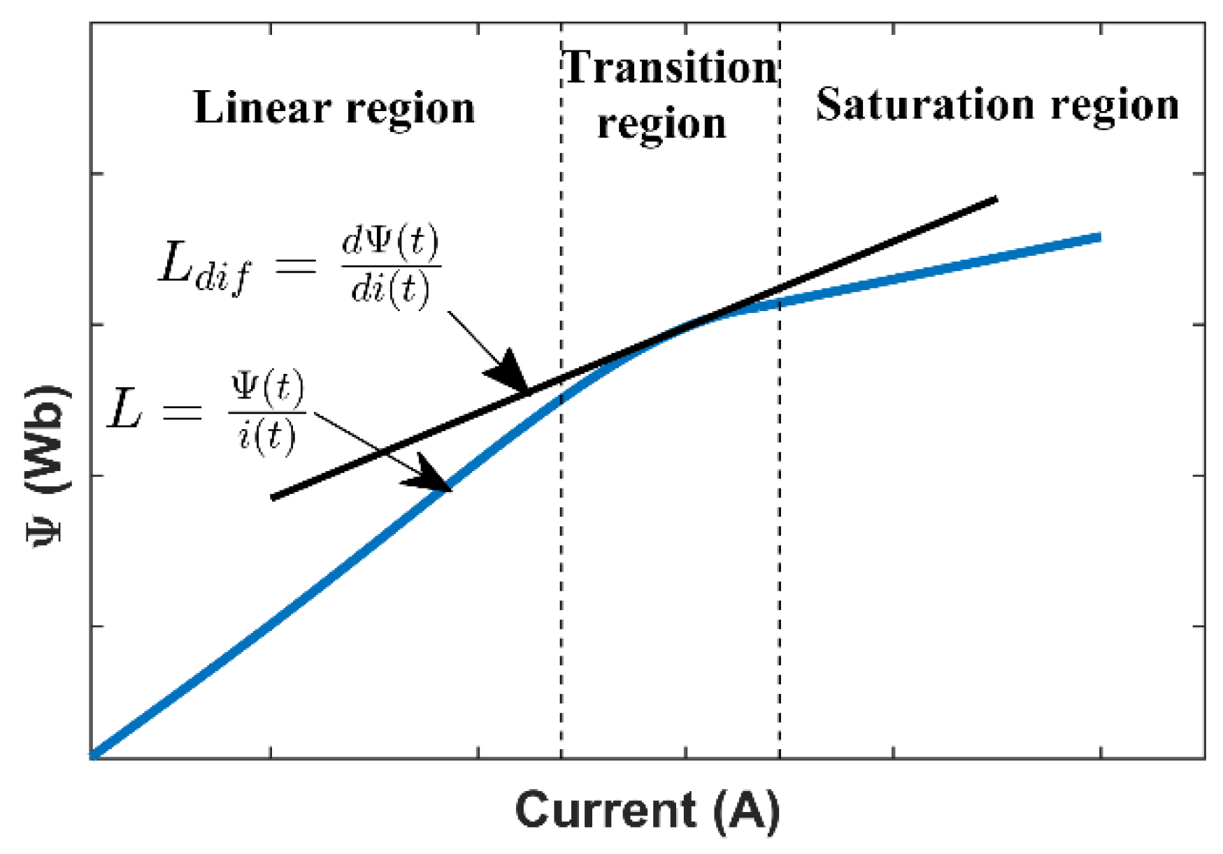
As it concerns the characterization of the inductor, the differential inductance, 𝐿_𝑑𝑖𝑓, is considered (Figure 1). It should be noted that the differential inductance is the slope of the total flux linkage ψ as a function of the magnetizing current [7].

$${\mathit{L}}_{\mathit{dif}}=\frac{\mathit{d} {\displaystyle \mathsf{\psi }}}{\mathit{di}}=\mathit{N}\frac{\mathit{d}\Phi }{\mathit{di}}$$

(1)

where N is the number of turns.

The saturation point represents a practical limit for the power electronic applications: it is defined as the current where 𝐿_𝑑𝑖𝑓 is halved to its rated value [7]. This definition is different from what manufacturers usually consider as the current limit operating point; indeed, in many cases, a drop of 10% of the inductance due to the current is considered. Recently, some manufacturers described the behavior up to a 30% inductance drop.

It is worth noting that 𝐿_𝑑𝑖𝑓 overlaps the inductance definition (meaning the ratio between flux and current) inside the unsaturated region. Unlike the linear zone, the inductance drop implies a higher current variation to obtain the same flux variation as when the inductor was operated in the linear region. The higher the current, the higher the losses will be, causing an effect of heating [32]. The increasing temperature generally reduces the current at which saturation arises [33]. The inductance (and permeability) drop is avoided by adding a small air-gap in the magnetic path [33]. Therefore, the permeability is kept fixed for a broad range, leading to a coil that has a lower dependence on the core rated permeability. A strategy to prevent deep saturation is increasing the cross-sectional area; however, it increases the weight and the cost, since a lower inductance requires more turns, increasing copper losses; hence, a trade-off is necessary [33]. In general, soft saturation ferrites are an alternative to materials with an air-gap core; for this reason, the models presented in this paper are discussed regarding this material.

Figure 1 shows a typical trend of the magnetization for increasing current. Based on this, three regions are identified. The linear region is characterized by constant inductance; this interval is commonly exploited for a maximum drop of about 10%. The transition region shows a monotonic decrease in the inductance, increasing the current; it is the region in which the operating range can be extended up to the point in which it is halved (or saturation point). Finally, the deep saturation is characterized by an almost constant flux implying a very low inductance value. The deep saturation zone is not of interest for power electronics applications, since the low flux variation corresponds to a low voltage at the inductor’s terminals, making it similar to a short circuit.

From the shape of the magnetization curve, it can be deduced that the characteristic curve of the inductor is expected to start with a constant line, then it decreases up to the deep saturation in which it is again constant, exhibiting a lower value compared to the rated one [7,10,11]. The two main analytical models considered in this paper are based on mathematical functions with a shape similar to the expected inductance value versus the current. It should be remarked that the inductance often shows a slight increase in the linear zone after the current increase from the null value. This part is exploited for operation near the discontinuous conduction mode (DCM).

The expected model is required to give the inductance value as a function of the instantaneous current flowing through the inductor; besides, other parameters, e.g., the temperature, can be taken into account.

$$L=L\left[I_L\left(t\right), T, \dots \right]$$

(2)

In the following, the arctan and polynomial models are analyzed in detail.

2.1. The Arctan Model

The arctan model has been proposed by [9]; it exploits the shape of the arctan function suitably adapted to the inductance curve. As a matter of fact, the arctan curve, increasing the independent variable, starts from a quasi-constant value, then it decreases until a lower constant value is reached. This curve also shows a continuous derivative. The identification of this model is based on the knowledge of four coefficients: L_nom, L_30%, L_70%, L_deepsat. L_nom is the nominal inductance of the inductor, L_30% and L_70% correspond to the drop of the nominal inductance of 30% and 70% caused by two currents labeled I_30% and I_70%, respectively. L_deepsat is the inductance value in deep saturation.

Based on these four parameters, the following coefficients have to be calculated:

$$\begin{array}{c}{\Gamma }_{30\%}=\frac{L_{30\%}-L_{deepsat}}{L_{nom}-L_{deepsat}}\\ {\Gamma }_{70\%}=\frac{L_{70\%}-L_{deepsat}}{L_{nom}-L_{deepsat}}\\ \sigma =\frac{cot\left(\pi {\Gamma }_{30\%}\right)-cot\left(\pi {\Gamma }_{70\%}\right)}{I_{30\%}-I_{70\%}}\\ I_L^{*}=\frac{ I_{70\%}·cot\left(\pi {\Gamma }_{30\%}\right)- I_{30\%}·cot\left(\pi {\Gamma }_{70\%}\right)}{cot\left(\pi {\Gamma }_{30\%}\right)-cot\left(\pi {\Gamma }_{70\%}\right)}\end{array}$$

(3)

The inductance is represented by the function:

$$L\left[I_L\left(t\right)\right]=L_{deepsat}+\frac{L_{nom}-L_{deepsat}}{2} \left\{1-\frac{2}{\pi } arctan\left\{\sigma · \left[i_L\left(t\right)-I_L^{*}\right]\right\} \right\}$$

(4)

The values of L_nom, and L_deepsat can be given from the manufacturer (datasheet and/or inductance curves); however, L_30% and L_70% have to be measured together with the corresponding current. Alternatively, two couples of values obtained for different currents, I_α% and I_β%, can be adopted, where α% and β% are the percentage reduction in the inductance from L_nom and range in the 10–90% range [9]. This model is an asymptotic model: L_nom is the asymptote of $L\left[I_L\left(t\right)\right]$ when $I_L\to -\infty$; that is approximated with the closest value of the inductance measurable at $I_L≌0$, and L_deepsat is reached for $I_L\to \infty .$

2.2. The Polynomial Model

The polynomial model has been proposed in [16,28]. It exploits the properties of a third-order polynomial function that, by suitable coefficients, shows a maximum and a minimum with an intermediate decreasing curve and can be used to reproduce the inductance versus current.

$$L\left[i_L\left(t\right)\right]={\displaystyle \sum }_{m=0}^3{L}_m ·i_L^m$$

(5)

The polynomial model can be identified based on the same parameters: L_nom, L_30%, L_70%, L_deepsat; however, better results can be retrieved by an augmented data set obtained by a measurement system. The coefficients of (5) are calculated by a least-squares regression (LSR). It should be remarked that not all the third-order curves can be used to represent the inductance, because it is expected that approaching the deep saturation value, the curve rises contrarily to the real inductance that must slightly decrease and then remains constant. On the other hand, the deep saturation is not interesting for power electronics applications.

2.3. Temperature Dependence

Both arctan and polynomial models allow encompassing temperature dependence. In this case, the expected behavior of the inductance is described by a family of curves parametrized with the temperature. These curves start from the same point at a small current and tend asymptotically to the same deep saturation value corresponding to the saturation. The higher the temperature, the lower the inductance will be in the intermediate part that must be suitably reproduced by the model.

The steps listed in the last sections have to be repeated for different temperatures of the inductor to be characterized, and thus, a family of curves is obtained.

In the arctan model, the temperature dependence can be considered by the coefficients σ and I_L*.

In the polynomial model, the dependence on the temperature can be described by modifying the polynomial coefficient

$$L\left(i_L,T_{core}\right)={\displaystyle \sum }_{m=0}^3{L}_m\left(1+{\mathsf{\beta }}_m{T}_{core}\right)i_L^m$$

(6)

Since the computational effort is proportional to the number of curves identified for each model, the comparison is performed for a unique temperature in this paper.

During the SMPS operation, evaluating the current profile within a switching period is of interest. Since the thermal constant of the inductor is much higher than this time interval, the inductor temperature can be assumed as constant. It should be remarked that the knowledge of the inductor temperature requires a thermal analysis since it depends on the power losses inside the inductor [15,16].

3. Inductor Characterization

3.1. The Test Rig

Since the two studied models need experimental values, a suitable DC/DC converter has been used to retrieve data from a non-linear inductor. Particularly, the LM5122EVM-1PH Evaluation Module (EVM) has been adopted (Figure 2). It is a synchronous boost converter adopting the Texas Instruments LM5122 synchronous boost controller IC. The circuit provides 24 V output at up to 4.5 A current with input voltage ranging from 9 V to 20 V. The switching frequency is set to 260 kHz as the default value. The board is equipped with a 10 µH SMD Flat Wire Inductor delivered by Wurth, code 74435561100, remaining linear up to about 9 A. The power MOSFETs are N-CH 40 V 100 A by NXP semiconductor PSMN4R0-40YS. The operation mode is set to “forced PWM”; other operations can be set to improve efficiency at light load [34]. For the purposes of this paper, the EVM has been equipped with the inductor MSS7341-103MLD by Coilcraft [35] as non-linear inductor. It has the same rated value of 10 µH of the original linear inductor, but its inductance is halved at a lower current, as can be deduced by the manufacturer’s data sheet. Additionally, the manufacturer gives the current values measured with a drop of 10%, 20% and 30% of the rated inductance. The two inductors are shown in Figure 3. The Wurth inductor has a volume of 3031 mm³ [36]; in this test, it has been replaced with the Coilcraft inductor chosen so that the maximum current imposed by the load causes a drop of 50% of the rated inductance. As a consequence, the core is smaller, corresponding to a volume of 206 mm³, meaning a reduction of about 93% [35]. From this, it can be noted that the exploitation of the inductor with a lower saturation current allows for a size reduction in the component and, therefore, a power density improvement of the converter. Finally, the performance of the converter in terms of the output voltage remains the same; as a second-order effect, a slight increase in the voltage ripple superimposed to the DC value could be appreciated.

3.2. The Inductor under Test

The MSS7341-103MLD inductor belongs to “shielded mount power inductor” series. It is a general-purpose ferrite inductor characterized by a low DC resistance and excellent current handling. Its rated value is 10 µH with 20% tolerance. The manufacturer provides the DCR resistance value (max 0.038 Ω) and the current, causing 10%, 20% and 30% drop of the inductance (Figure 4). These values allow a rough estimation of the value at which the inductance is halved, meaning the saturation. Considering the rated value of 10 µH, it is halved at about 2.35 A. It should be remarked that the DC current causing the inductance drop is given at 25 °C and that the fitted curve loses its accuracy increasing current after the saturation value. A dedicated experimental characterization will allow identifying more precisely the inductor behavior, as explained in the following.

3.3. Inductance Measurements and Characterization

The inductor MSS7341-103MLD has been characterized by using the same EVM-1PH board. It has been mounted replacing the linear inductor. In order to obtain the points corresponding to the inductance for a given current, a load allowing a large current ripple to span all the operating range up to deep saturation has been connected. In particular, a load of 28 Ω allows, in a time interval defined by the conduction time of the power switch, a current variation starting from a very low value (near the discontinuous limit) up to about 4.5 A, corresponding to deep saturation. The EVM board has been suitably modified to connect a different inductor and the current probe; it is provided by Tektronics, model TCP0020. The current profile has been sampled, and the differential inductance has been calculated following the approach described in [10].

The differential inductance is calculated as:

$${\mathit{L}}_{\mathit{dif}}=\frac{{\mathit{V}}_{\mathit{L}}}{\mathit{di}/\mathit{dt}}$$

(7)

where V_L is the voltage applied to the inductor that, for a boost converter, coincides with the supply voltage V_s, and is constant during T_ON. The current slope is calculated based on an LSR performed on a set of 50 samples at a time, and this differential inductance value is associated with the current mean value calculated on the same samples. Repeating the calculation on the whole set of samples, the characteristic curve of the inductor is obtained. A picture of the test rig for measurement is shown in Figure 5. The current acquired by the oscilloscope flowing through the inductor is shown in Figure 6; it can be noted that the slope of the current starts with a constant value, then it increases (corresponding to a lessening of the inductance) until it reaches the deep saturation where the slope remains constant despite the further increase in the current, as expected. The top trace, labelled CLOCK, is the internal clock reference signal accessed by the pin “SYNC” of the EVM, it has the frequency of the PWM carrier but out of phase with respect to the state of the switch. The current has been sampled with a sampling time of 1 ns obtaining a vector of 1920 samples and a vector of 38 points representing the inductance has been obtained (the time interval in which the current is sampled is one-half of the period corresponding to a frequency of 260 kHz, meaning 1.92 µs). From this dataset, both the arctan model and the polynomial model can be identified.

The inductor characterization has been performed at the environmental temperature (that coincides to the one specified by manufacturers) and the two models have been calculated with these data. Since the data are acquired based on a few switching periods (in our case, about 40 µs are sufficient to sample ten periods of the current waveform), no appreciable rise in the temperature is noticed. As a matter of fact, the thermal constant is much higher than the electric constants of the circuit, and the effect of the temperature requires some seconds to be appreciated.

4. Analysis and Comparison

Three different tests have been conceived to compare the performance of the two studied models: firstly, based on the data coming from the test rig, the model is identified by retrieving the inductance versus the current curve; then, a current profile is evaluated by using the identified models, and finally, the two models are implemented by Micro-cap Spice software to simulate a boost converter. The proposed analysis encompasses the simulation time. While both measurements and model identification are performed once for given temperature, the current profile calculation, aimed to estimate the maximum value, in some applications must be performed in real time during the switching time. With the use of modern fast switching devices such as those based on SiC or GaN, the switching time is progressively reduced; it represents a constraint on the choice of the microcontroller.

4.1. Identification of the Characteristic Curve

The characteristic curve is identified using both approaches based on the arctan and polynomial models.

As it concerns the arctan model, firstly, the L_nom, L_30%, L_70%, and L_deepsat are extracted. The following values are obtained: L_nom = 11.3 µH; L_30% = 7.91 µH; L_70% = 3.39 µH; L_deepsat = 1 µH; L_30% and L_70% correspond to a current of 2.24 A and 3.07 A, respectively. Then, the characteristic parameters (3) are calculated; finally, by Equation (4) the characteristic curve can be plotted. The time required to retrieve the parameters (3) has been calculated by the function “tic” and “toc” by MATLAB^® (version R2014b has been used in this paper). A time of 0.142 µs has been required (for the sake of precision, each calculation is repeated 1000 times, and the result is divided by 1000, the final results is calculated as a mean value of several tests; in the computer, only MATLAB software is running during calculation). A vector containing the current is built to obtain the characteristic curve L(i). It contains 6001 samples from 0 to 6 A with a step of 1 mA. The inductance is evaluated by (6) for each current point and then it can be plotted. The time required to calculate the inductance was 474 µs.

The polynomial model directly uses the sampled values of the current to perform an LSR with a third-order curve. The function “polyfit” is used to calculate the polynomial coefficients. This calculation required 19.425 ms. The polynomial coefficients are: L₃ = 0.0069 × 10⁻⁴, L₂ = −0.0495 × 10⁻⁴, L₁ = 0.0564 × 10⁻⁴, and L₀ = 0.1253 × 10⁻⁴. It can be noted that the rated value of the inductance measured at low current and corresponding to the coefficient L₀ gives a higher value compared to the rated one.

Finally, the inductance is calculated using the same vector of current data values used for the arctan model; this calculation needed 50 µs.

The curves corresponding to the two models are shown in Figure 7.

The obtained curves show that the polynomial curve can model the initial part in which a slight increase is present; however, it cannot be used approaching deep saturation since it shows an increase in the inductance. The arctan model approximates the values corresponding to deep saturation for higher current; however, the decreasing value asymptotically follows the deep saturation value. Both models can cover the whole range of operation, meaning from a small current up to saturation. This last consideration improves what was stated by [26], which showed the polynomial approximation validity for a reduced range of currents.

4.2. Current Profile Evaluation

The current flowing through the inductor impacts the electromagnetic interference generated by the converter. To be commercialized, an SMPS must comply with standards; for this reason, the design of a suitable filter is mandatory, and it influences the power density of the whole converter [37,38,39,40].

The inductor model is useful for the calculation of the current profile when employed in a DC/DC converter. In particular, in a boost converter, during T_ON, the voltage applied to the inductor is constant, and the current is given by the constitutive equation in which the inductance depends on the current:

$$v_L\left(t\right)=\frac{d\mathsf{\Phi }\left(i_L \right)}{d{i}_L}·\frac{d{i}_L\left(t\right)}{dt}=L\left(i_L\right)\frac{d{i}_L\left(t\right)}{dt}$$

(8)

It is convenient to discretize (8) to calculate the current samples. In this case, the current is retrieved using the arctan and the polynomial models starting from the same maximum value and proceeding backward until finding the minimum. Obviously, it is also possible to start from the minimum value; however, due to the non-linearity of the inductor, it is unknown a priori. In addition, the maximum value is a design constraint since it is imposed by the inductor.

$$i_L\left(k+1\right)=i_L\left(k\right)+\frac{v_L\Delta t}{L\left(i_L\left(k\right)\right)}$$

(9)

It should be remarked that a different method to retrieve the current is proposed by [9]; we solved Equation (9) using the two models, since its implementation is straightforward.

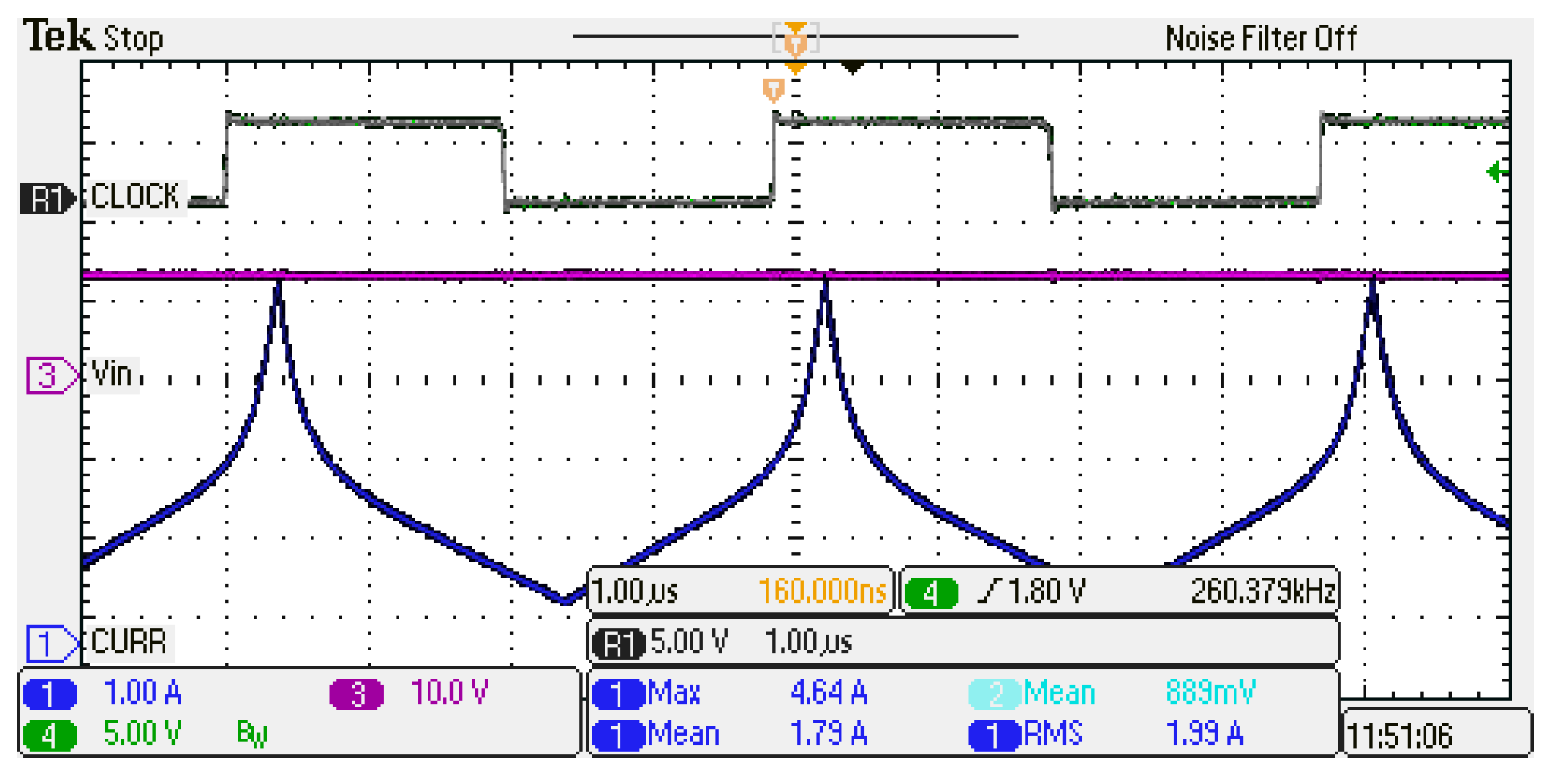
As a reference for the simulations, we consider a real situation: a screenshot of the oscilloscope is given in Figure 8, where it can be noted that the maximum value of the current assumed as the starting point is equal to 2.68 A; it corresponds to the saturation point. The top trace, labelled as CLOCK, is the internal reference signal accessed by the pin “SYNC” of the EVM, it is out of phase with respect to the switch state.

The current profile calculated by (9) adopting the two models is shown in Figure 9; it encompasses the measured values as well. It can be noted that the two curves give similar results, as it is demonstrated by the absolute error curves given in Figure 10. The time required to solve (9) by the arctan model was 131 µs, whereas the polynomial model required 121 µs.

The knowledge of the current profile is useful for calculating its root mean square that can be employed for the input differential mode filter design [37]. The use of this devices allows the standards compliance, and usually, its sizing is influenced by the non-linear behavior of the power inductor [17]. Besides aiming to optimize the power density of the converter, the input filter must be taken into account [38,39]. It should be remarked that, differently from an SMPS employing a linear inductor in which the RMS value of the current can be easily calculated, to evaluate the RMS value with a non-linear inductor, the inductor differential equation needs to be solved or simulated using the inductor model. From the obtained values of the AC RMS current (

Table 1. Comparison of characteristics parameters of the current.

	Model
	Arctan	Poly	Experimental
DC RMS [A]	1.6388	1.6276	1.7
AC RMS [A]	0.6435	0.6019	0.574
MEAN [A]	1.5071	1.5122	1.6
RMSE	2.0042	1.7525	-

), it can be noted that there is a slight overestimation for both models; it does not represent a problem in filter design where a safety limit is taken into account [41]. The root-mean-square error (RMSE) is slightly higher for the arctan model.

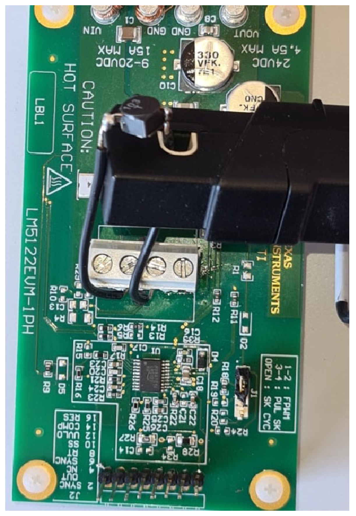
4.3. Simulation of a DC/DC Converter with Non-Linear Inductor

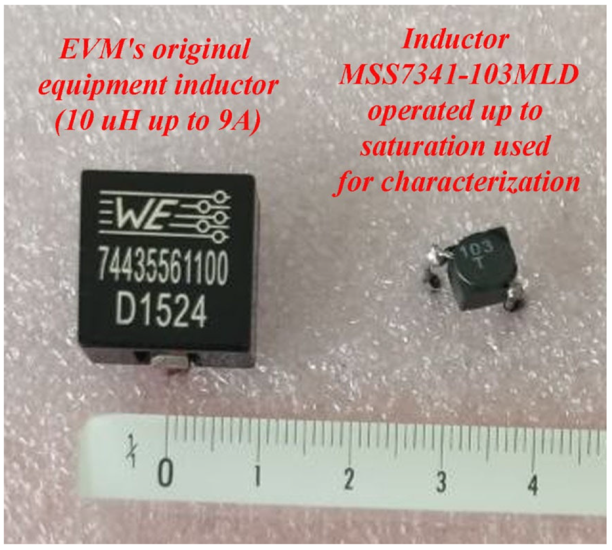
The DC/DC boost converter implemented in the LM5122EVM-1PH Evaluation Module (EVM) is analyzed by SPICE simulation in a Micro-Cap simulator. There are two implementations of the non-linear inductors in the Micro-Cap simulator. The first involves a behavioral model in which the inductance is implemented, specifying an expression involving time-varying variables for the inductance (or flux). The other one is a hysteretic core model based on the Jiles–Atherton model. 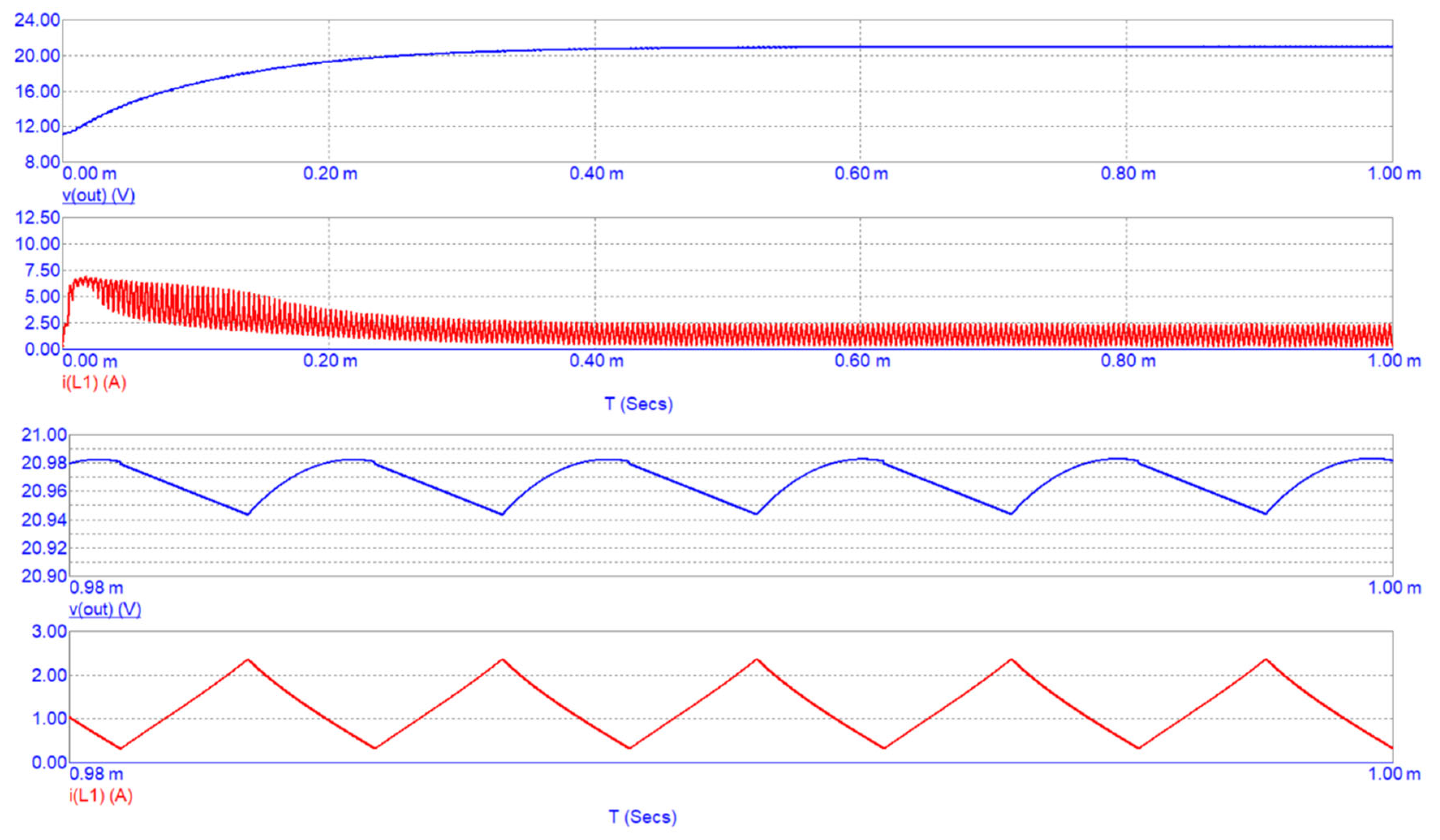For this paper, the first built-in non-linear inductor model is exploited, by implementing Equations (5) or (6) for the arctan and polynomial characteristics, respectively, as shown in Figure 11 and Figure 12. The simulation of a 1 ms transients resulted in similar current profiles with a good correspondence for both simulations and experimental measurements (gate voltage at 260 kHz with a duty cycle of 50%). The simulated current profiles through the non-linear inductor are reported in Figure 13 and Figure 14. Regarding the simulation performance, both simulations were carried out with a maximum time step of 2 ns and a run time of 1 ms; the polynomial model allows for a 15% faster simulation resulting in a simulation time of 5.10 s against the 5.88 s of the arctan, due to lower number of sums and multiplications required for the arctan model.

5. Discussion

The model identification of power inductors operated in the non-linear zone needs a dedicated measurement setup since, usually, manufacturers do not give the necessary information. By the test rig, the differential inductance has to be measured in different operating points characterized by a DC current and AC variation superimposed. Each characterization has to be performed at the same temperature. The arctan model requires four parameters; the rated inductance and the deep saturation value can be deduced by the manufacturer’s data sheet or by inductance curves; differently, the inductance corresponding to a drop of 30% and 70% have to be measured. The percentage values are not critical, and a different couple of values can be used; however, since the current at which the inductance is obtained is not known a priori, it has to be searched for among the interval of the allowed current. Four measurements can also identify the polynomial model; however, increasing the number of samples can improve its accuracy. Based on this, the measurement effort for both models is similar. After data acquisition, both models require parameter calculation. The calculation is significantly faster for the arctan model. Indeed, the polynomial model requires the use of “polyfit” MATLAB^® function or a similar tool that is more time-consuming; nevertheless, this calculation is performed only once for a given temperature.

The inductance curves obtained by the models show that the polynomial curve can model the initial part in which a slight increase is present; however, it cannot be used in proximity of deep saturation, since it shows an increase in the inductance. The arctan model also approximates the values corresponding to deep saturation for higher currents; however, the decreasing value asymptotically follows the deep saturation value. Both models can describe the inductor behavior in the whole range of operation, meaning from a small current up to saturation.

Regarding the inductance curve calculation based on a current vector, the polynomial model was notably faster (50 µs against 474 µs); it is due to the simpler polynomial model requiring only a limited number of sums and multiplications compared with the arctan model. The polynomial model allowed us to avoid implementing power elevation since each power can be considered as multiple product; differently for the arctan calculation, the MATLAB^® library has been used. As a consequence, this calculation time could be reduced for both models by optimizing the algorithm directly into the microprocessor or DSP.

As concerns the current profile calculation, obtained by the resolution of (8), a similar computation time has been noticed.

Finally, performing a SPICE simulation of the whole DC/DC boost converter employing the non-linear power inductor, the polynomial model allows for a 15% faster simulation resulting in a simulation time of 5.10 s against the 5.88 s of the arctan model.

A summary of the computation time results are given in

Table 2. Computation time comparison.

	Arctan	Poly	Note
(1)  Identification of the characteristic curve
Measurements			Both methods need a measurement setup.
Model Parameter calculation	0.142 µs	19.42 ms	Required only once.
Inductance vs. current calculation	474 µs	50 µs	The inductance is evaluated based on a current vector of 6000 points.
(2)  Current profile evaluation	131 µs	121 µs	Obtained by solving differential equation in discrete form.
(3)  Micro-Cap Spice simulation	5.88 s	5.10 s	Simulation of a Boost DC/DC converter implementing the non-linear model of the inductor with a simulation time of 1 ms.

.

6. Conclusions

Two analytical models for power inductors operated up to saturation have been compared. Both models are based on functions that reproduce the shape of the inductance versus the current, meaning the arctangent and a third-order polynomial curve.

The comparison has been based on the same inductor and experimental setup. Performance is compared from different points of view, considering the characteristic curve identification, a current profile calculation, and a simulation of a DC/DC converter employing the non-linear inductor.

Both models are able to reproduce the inductance curve in the main operating region, i.e., when the current approaches saturation. The polynomial model can reproduce an increase in the inductance when the current increases from a small value, but it is unable to reproduce the behavior after the deep saturation point. The arctan model shows a slightly decreasing trend when the current increases from a small value, but the deep saturation behavior is also well reproduced for higher currents. This last feature is helpful in the simulation when high current peaks can be reached during the start-up phase. In fact, the deep saturation value of the inductance is reached asymptotically; however, it does not represent a problem in practice. From the point of view of the computation time, the inductance calculation employing the polynomial model is faster.

The current profile evaluation showed similar computation time and accuracy results. The AC RMS value is significantly well calculated since it is helpful for EMI filter design.

Finally, the simulation of a DC/DC converter adopting the described models showed satisfactory results in reproducing voltages and current for the two models, confirming the goodness of both. The simulation time was 15% faster employing the polynomial model.

In conclusion, both models performed well in reproducing the electrical parameters in a circuit; the polynomial model exhibits shorter computation times, whereas the arctan model guarantees the correct operation outside the current operating range.