1. Introduction
The ORGAD is a Hybrid S-Band (2856 MHz) RF-Photo injector operating at the Schlesinger Compact Accelerator Center in Ariel University, providing a relativistic electron beam with beam parameters of 6.5 MeV kinetic energy, 300 pC of pulse charge and 150 fs electrons pulse duration [
1,
2]. The Hybrid RF-Photo injector has a novel structure of 3.5 standing wave (SW) cells and nine traveling wave (TW) cells in a single RF cavity. The SW section accelerates the electrons while the TW cells bunch the electron beam via a negative chirp applied. The electron beam is used to drive a super-radiant THz FEL, using a 90 cm undulator emitting coherent THz radiation at 1–3 THz [
3,
4], as well as other beam driven applications [
5,
6,
7]. Super-radiant FEL emission requires high quality beam [
8,
9,
10].
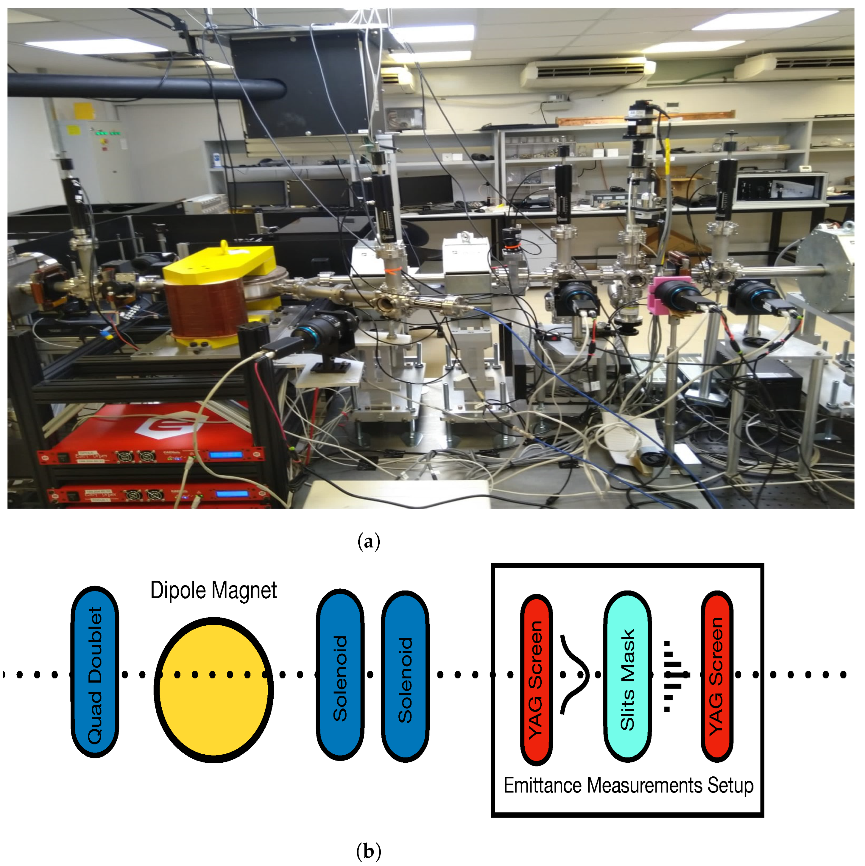
An important beam property is the beam normalized emittance that provides insight of the beam divergence rate and the angular distribution of the charged particles. The experimental emittance measurements will be conducted using a multi-slit mask, consisting of an 11 slit tungsten mask with a slit width of 0.04 mm, slit separation of 0.65 mm and thickness of 2.2 mm. The mask will divide the electron beam into several beamlets, each with a significantly lower charge than the original beam, and therefore their divergence will be dominated by the emittance property while the space-charge effects will be diminished to a negligible level. In order to measure the beamlets after the mask, we will use a YAG (Yttrium Aluminium garnet) crystal and Images will be taken using a Basler camera equipped with a 100 mm NIKKOR macro lens directed to a rear mirror, reflecting the luminous YAG crystal towards the camera. The image processing and analysis is performed using a dedicated Matlab script, which interfaces with a LabVIEW program. A user interface was rigorously designed and built to mitigate the complex process of emittance computation. The entire process is fully automated and user-friendly.
Prior to the experimental measurement, a simulation is performed using the LabVIEW script with a built-in Matlab emittance calculation code. To test the algorithm, we use a GPT exported mock beam image, which is then converted to a matrix and sent to the algorithm as an input beam, where its emittance is calculated and compared with the value obtained from GPT.
2. Multi-Slit Based Emittance Measurement Simulation
Emittance is a particle beam property that describes the mean divergence of a beam with respect to its propagation in phase space, where momentum and position are its coordinates. Transverse emittance defines the divergence of a particle beam compared with propagation on the optical axis. There are several methods to measure particle beam’s emittance [
10]. Most familiar methods are the quadruple scanning [
11] and pepper-pot techniques [
12].
Executing a single shot transverse emittance measurement using the quadruple scan technique is not feasible since the process combines a large number of pulses, each with a different magnetic field. Therefore, the quadruple scan does not comply with the demand of measuring the transverse emittance using a single shot. The pepper-pot technique can be used to obtain the transverse emittance with the same measurement process as the multi-slit technique only for a large amount of charge, since the beamlets passing via the holes has a very small charge in each, due to the small holes cut in the mask. The pepper-pot technique’s advantage is that one obtains dual-axis emittance in a single shot, but a low image resolution makes it much harder to optimize and calibrate [
13].
The method described in this publication is the multi-slit technique in which an electron beam passes through a Tungsten slit-mask and gets divided into beamlets. The beamlets, unlike the main electron beam before passing through the slit-mask, are emittance dominated due to significantly reduced charge, and when they hit the YAG crystal, a luminous multi-Gaussian pattern will emerge [
14]. Since the slit separation is larger than the slit widths, there is no constructive nor destructive interference. This fact allows us to measure each beamlet separately, calculate its size and divergence, and finally calculate the normalized emittance value.
The multi-slit technique takes into account the change in transverse position of each electron upon passing from the slit-mask to the YAG crystal. This divergence is calculated by dividing the beamlet’s transverse position difference in the initial (mask) and final (YAG) states by their distance from each other.
where
is an integer corresponds to the beamlets order and
w is the spacing constant between the slits. Therefore,
is a transverse position in the mask,
is the YAG crystal’s beamlet position on the YAG screen,
L is the distance between the two and
is the beamlet divergence. Since we use image analysis, we translate the number of particles (electrons) into intensity. Since each beamlet has a transverse Gaussian density pattern, a Gaussian fit is applied on each beamlet to extract the RMS beam spot size. Similarly to Equation (
1), the RMS divergence
can be calculated using the obtained RMS spot size.
where
is the RMS spot size and
is the RMS divergence of the beamlet. The experimental transverse emittance measurement system is located approximately 83 cm from a dipole spectrometer (see
Figure 1), where two steering coils and two focusing coils installed at this part are used to collimate the beam and control its transverse size and position.
3. Simulations Based Analysis
Initial analysis is performed using GPT (General Particle Tracer). A 3D charged-particle beams simulations which provides information about the particle beam characteristics (including emittance and space-charge effects), and external fields dynamics. In this research GPT simulates the propagation of a Gaussian electron beam throughout the hybrid accelerator. This start-to-end simulation (starting from the cathode) includes all of the electron-optics elements such as solenoid coils and a dipole spectrometer. GPT provides the beam parameters and is also used to export a mock image, which is used to verify the obtained analysis results. This is similar to an experiment, where a LabVIEW script imports an image from the camera and converts it into a matrix, in order to process the image. The data obtained from GPT is then sent to the LabVIEW code as an image produced by a camera (later this will be an actual image from the diagnostics cameras in the beam-line), a Matlab script analyses the image and identifies the results pattern, calculates the normalized emittance, and sends it back. We have added a LabVIEW-based GUI which is controlling and providing the user with the necessary results in a clear manner.
Figure 2a shows the transverse beam distribution obtained using the mock beam from GPT. To demonstrate the Gaussian form of the beam, we plotted a profile of the transverse beam distribution compared with a standard Gaussian fit (
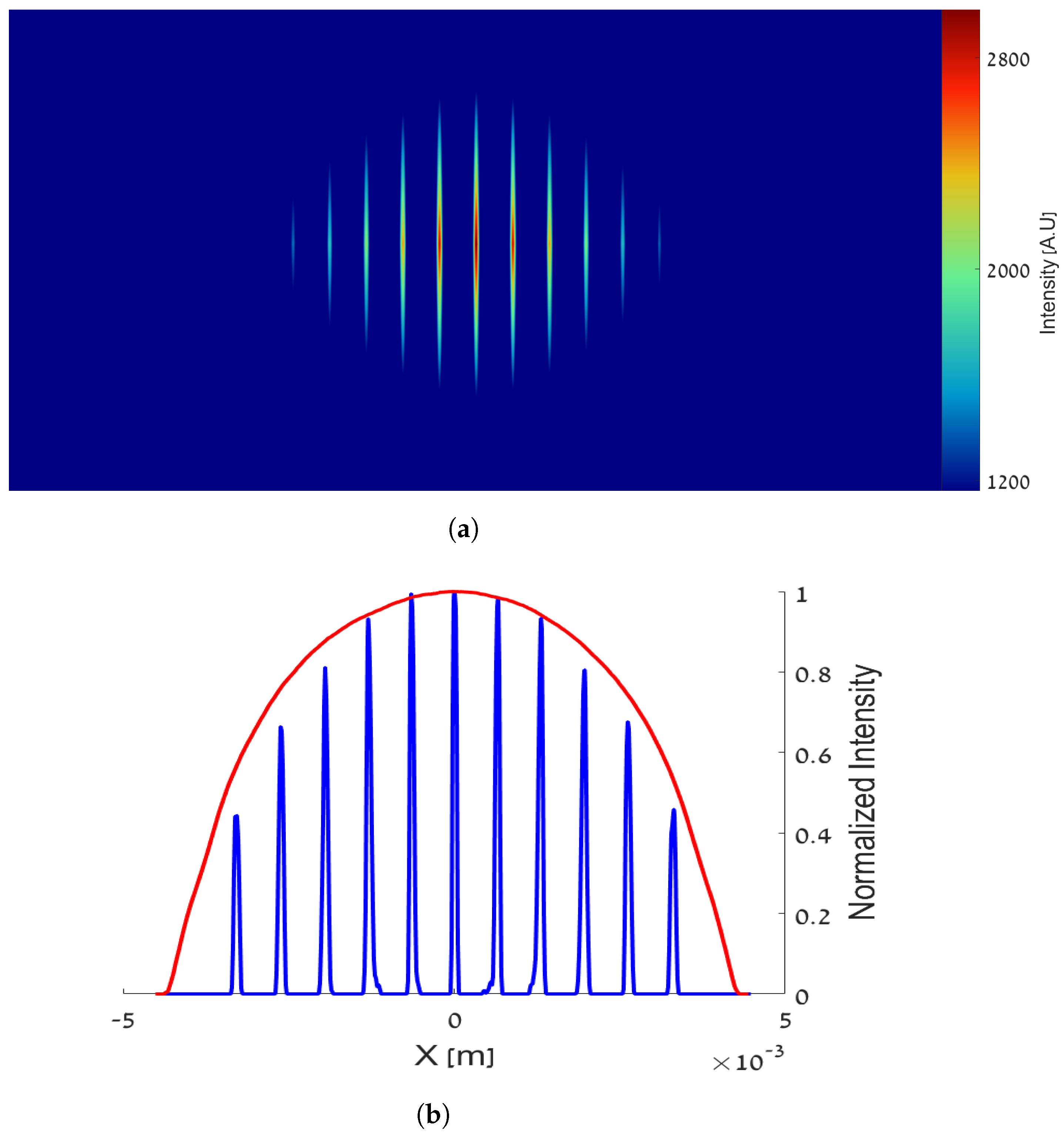
Figure 2b). This beam then passing through the slit-mask and get separated into beamlets as shown in
Figure 3a. When obtaining a mock image from GPT, the first step is converting the image into a processable graph. This step is demonstrated in
Figure 3, where at the right side is the initial plot obtained using the conversion from a particles density plot into a continues one. Note that the envelope of these sharp Gaussian peaks has a Gaussian form as well, since the main beam is a Gaussian one.
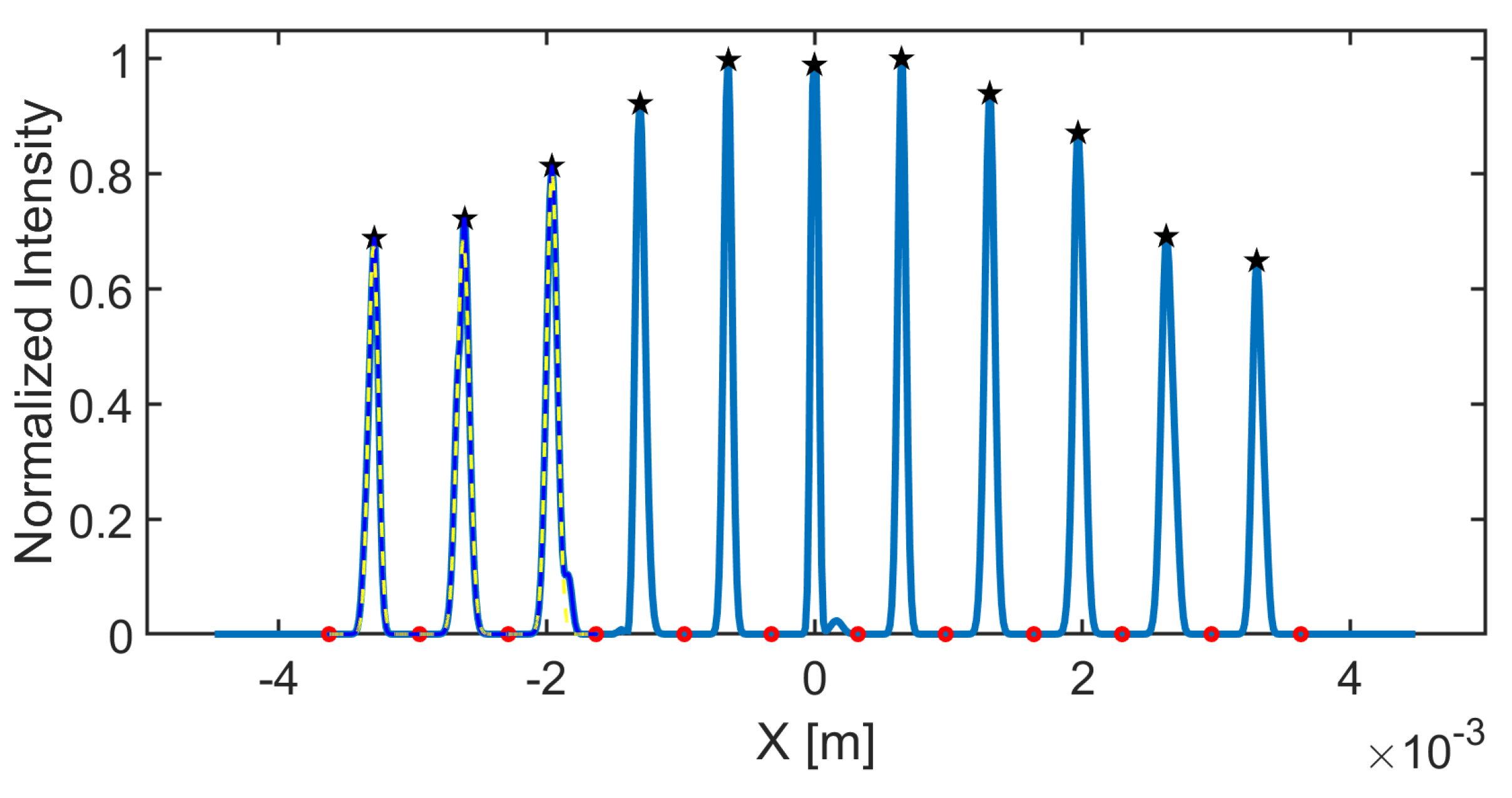
Figure 3b is smoothed to verify the right peaks and borders of each beamlet are used in the emittance calculation, providing accurate estimation of the normalized emittance. The smoothing is applied using a series of multi-Gaussian fits. The result of each multi-Gaussian fit is analyzed by the algorithm, and eleven even-spaced peaks are identified. The even-spaced peaks correspond to the Tungsten slit-mask, which consists of eleven slits. Next, the borders and the peak of each beamlet are marked with red circles and black polygons. Afterwards, a single Gaussian fit is implemented on each beamlet. By applying this fit, we obtain a numerical value of the standard deviation, which is interpreted as the RMS spot size (see
Figure 4).
The RMS spot size provides information about the divergence of the beamlets. The detected beamlets at the YAG crystal are wider than the slit width, hence we need only the detected beamlets coordinate to find their RMS divergences. In other words, we use the RMS spot size obtained from the single Gaussian fit to obtain the beamlets RMS divergence using Equation (
2).
Using the above variables, one can calculate the transverse emittance, by calculating the second moments
and
and their correlation
using Equations (
3)–(
6). These equations use the intensity of the beamlet, the normalized position and divergence coordinates [
11,
15].
where
is second moment of the transverse position,
is second moment of the transverse divergence, and
is their correlation term. To ensure that the profile of the main beam is conserved after splitting into beamlets by passing the slit-mask, a comparison was executed by taking the profile of the main beam and compare it with the profile of the beamlets. The comparison is shown in
Figure 5b showing good fit with the envelope of the beamlets. We have added, an intensity distribution plot to demonstrate that the middle beamlet contains the highest intensity, or amount of particles, while the lateral contains the lowest intensity, or amount of particles (see
Figure 5a).
Six independent GPT simulations are analyzed here. Each beam contained a different total amount of charge and the simulated trajectory is the path from the cathode to the YAG crystal. Six images, similar to image in
Figure 3a, were imported into the Matlab script performing the procedure described previously in order to estimate the deviations between simulations and the precision with respect to the value obtained from GPT. Since GPT’s emittance calculation takes into account each and every particle’s displacement in the beginning and the end of the simulation, it can be considered as a valid reference for comparison.
4. Simulation Results
GPT simulations provide the normalized emittance and the Lorentz factor
. In all six simulations considered here,
has the same constant value of 13. Since the gun accelerates the electrons to relativistic velocities, it is approximated that
:
The tables below compare the slit analysis with GPT by showing the normalized emittance results obtained for each case and the deviation between these results. Processing time was measured and compared as well. The process includes the multi-Gaussian fit, single Gaussian fit, extracting the RMS values, normalized emittance calculation, and a plot display of each step. The difference between the first two simulations is the initial transverse emittance. Both simulations used the same charge (300 pC). In the other simulations, we defined same transverse emittance, but varied the charge. The number of macro particles for all the simulations was set to
particles, pulse length was the same, and space charge effects were included. The deviations between the results are obtained by calculating the absolute difference between GPT’s normalized emittance to the calculated one, and dividing it by GPT’s normalized emittance (see Equation (
8)).
Table 1 presents the obtained results from six different simulations including the deviations between the transverse emittance obtained from GPT and the calculated transverse emittance obtained using the algorithm. Approximately
deviation in all simulations were obtained.
From
Table 2, note that the measured simulation time is long due to a large number of figures plotted during the process, where canceling them will significantly reduce the processing duration.


