1. Introduction
A large number of scientific problems are often ascribed to the problem of solving Boolean equations. Research on quantum algorithms for solving nonlinear Boolean equations in binary fields is a critical problem in computational mathematics, cryptographic, design, and analysis.
Feynman first proposed the concept of a “quantum computer” in 1981, pointing out that only a quantum computer can effectively simulate a quantum system. In 1985, Deutsch proposed the Quantum Turing Machine for the first time and designed the Deutsch algorithm [
1], which laid the basic idea for a quantum algorithm. In 1992, Deutsch and Jozsa jointly proposed the Deutsch–Jozsa algorithm [
2], which was the first time exponential acceleration of a classical algorithm was achieved. The Shor algorithm proposed by Shor [
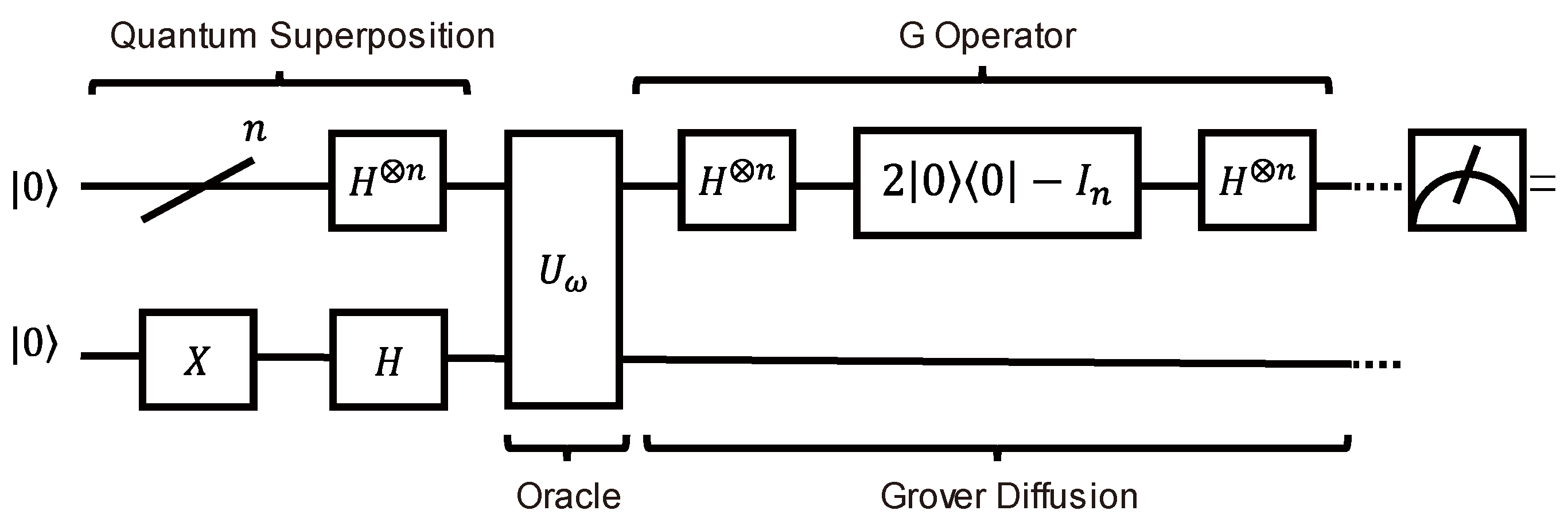
3] in 1994 could solve the core large prime factorization problem in an RSA cryptosystem with polynomial time complexity and had better performance at an exponential level compared with classical algorithms. In 1996, Grover proposed the Grover quantum search algorithm, which could search for targets in an unsorted database with a time complexity of
[
4,
5,
6,
7].
In recent years, more scholars have devoted themselves to quantum algorithm research with the development of scientific theories on quantum computing. They have obtained many valuable findings, such as the problem of solving polynomial systems with noise, integer factorization problems, and knapsack problems. The Grover algorithm can further generalize the problem of solving Boolean equations and expand it to the search problem of finding a target in the solution space of equations. Younes et al. [
8] proposed a hybrid quantum search engine. When the number of solutions in the search space exceeded N/3, the algorithm’s time complexity was O(1). Zhou et al. [
9] optimized the Grover algorithm by changing the phase rotation angle. When the number of solutions in the search space exceeded N/4, the target solution could be found with a success probability of no less than 98.01% in only one search in the search space. When the number of solutions in the search space equaled N/2, the probability of being found was 1. Zhu et al. [
10] developed a robust quantum search algorithm based on the Grover–Long algorithm, with the same time complexity as the Grover algorithm and a high tolerance for M/N uncertainty. In [
11], by adaptively changing the search space of different target component proportions, the Grover algorithm achieved overall improvement in the probability of success. Liu et al. [
12] proposed a new method of integer factorization based on the Grover search algorithm. Zhang et al. [
13] solved the problem of route planning for two manipulators based on the Grover algorithm. Xie et al. [
14] proposed an improved quantum search algorithm and applied it to solve the kernel properties of rough sets, which improved the probability of the target component as a whole. Hou et al. [
15] proposed an algorithm that leveraged the quadratic speed-up offered by the Grover search to achieve a quantum algorithm for the knapsack problem that showed improvement from classical algorithms. Ju et al. [
16] showed how quantum Boolean circuits could be used to implement the oracle and the inversion-about-average function in Grover’s search algorithm and proposed a template of quantum circuits that was capable of searching for the solution of a certain class of one-way functions. Harrow et al. [
17] proved that any classical algorithm for solving linear systems of equations generically required exponentially more time than our quantum algorithm. At present, the main problems faced by using the Grover algorithm to solve Boolean equations are still the depth of the quantum circuit and the probability of quantum states.
IBM Qiskit [
18,
19,
20,
21,
22] is an open-source quantum-computing framework that provides basic qubits, quantum logic gates, and quantum simulators on which quantum circuits and various quantum algorithms can be simulated. In this paper, we use the IBM Qiskit framework to simulate the quantum circuit of a Grover algorithm, solve Boolean equations of different variables, and prove the feasibility of the Grover algorithm in solving the equations. The experimental results show that the solutions of the equations can be found with a high probability when the number of variables is smaller than 21.
Section 2 presents the main steps of the Grover algorithm and the characteristics of nonlinear Boolean equations in a binary field.
Section 3 introduces the principle of converting Boolean equations into the quantum circuit and uses the Grover algorithm to solve Boolean equations on this premise.
Section 4 optimizes the quantum circuit for solving Boolean equations from three aspects: classical algorithm preprocessing, ancilla bit multiplexing, and the uses of a phase quantum gate.
Section 5 introduces the experimental results of solving Boolean equations with different variables, as well as the relationship between the number of variables, the depth of the circuit, and the number of qubits, and analyzes the experimental results.
Section 6 concludes this paper and gives an outlook on future work.
3. Simulation of the Grover Algorithm Based on the Qiskit Framework
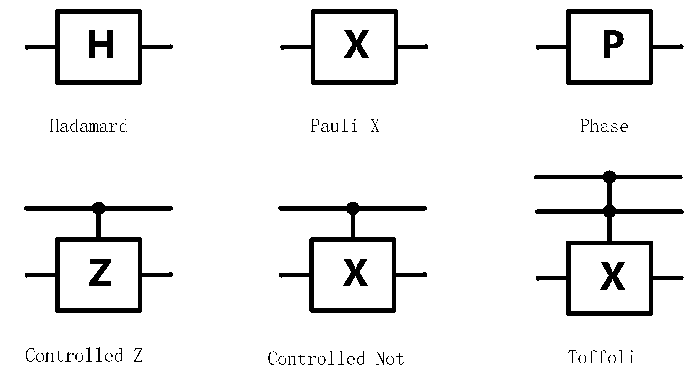
Qiskit is an open-source quantum-computing framework developed by IBM with essential quantum bits providing various quantum simulators, quantum algorithms, and quantum gates, such as the H gate, Pauli-X gate, CZ gate, CNOT gate, Toffoli gate, and Phase gate, as shown in
Figure 2. Qiskit also provides a Python API that can program and simulate quantum algorithms on classical computers.
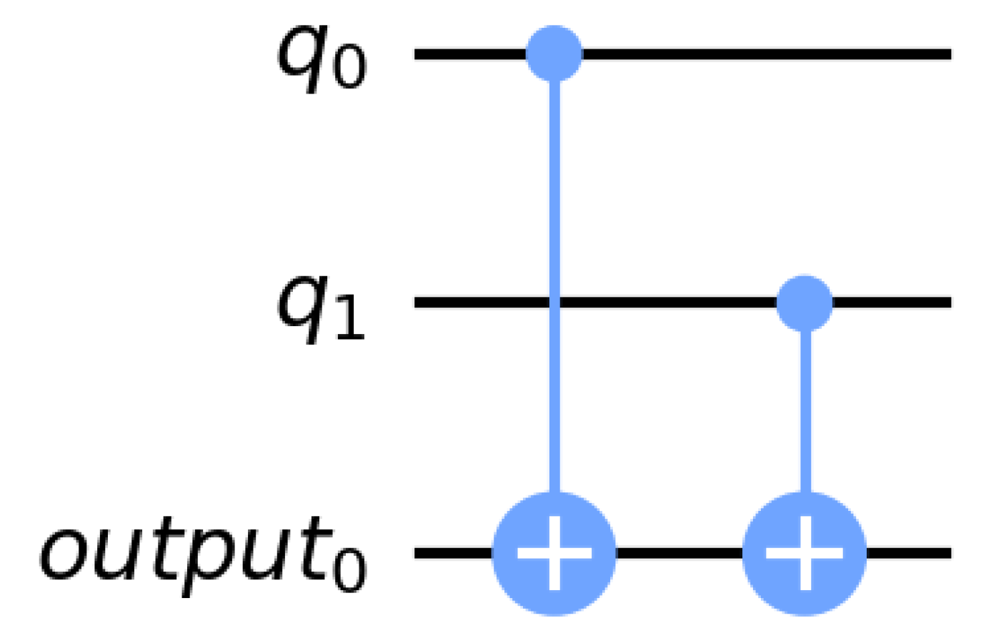
In this paper, we used Qiskit to simulate the Grover algorithm on the Jupyter Notebook, tried to discover the implementation of the algorithm on Boolean equations, and built a quantum circuit for the Grover algorithm to solve the equations. As shown in
Figure 3, when building a quantum circuit, according to the characteristics of Boolean equations, the addition operations of the Boolean equations are equivalent to the XOR operation in the Boolean logic relationship, which can be simulated with two CX quantum gates on the quantum circuit.
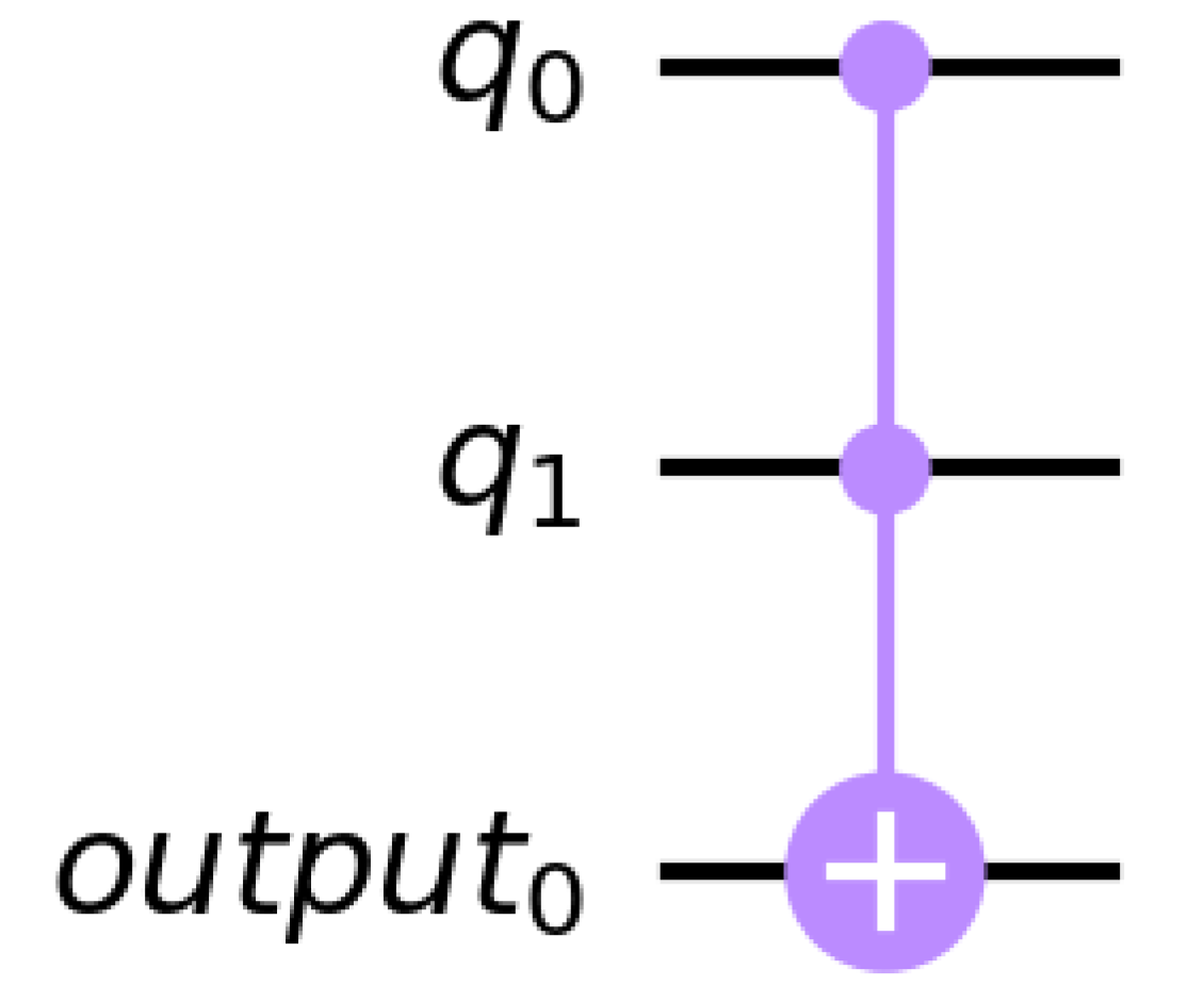
As shown in
Figure 4, the multiplication operations of the Boolean equations are equivalent to the AND operation in the Boolean logic relationship, which can be simulated with a CCX quantum gate on the quantum circuit.
In this paper, the combination of two CX quantum gates was called the XOR element, and one CCX quantum gate was called the AND element. The oracle part of Boolean equations could be composed of both XOR and AND elements. This way of expressing Boolean equations on quantum circuits provided feasibility for solving the equations.
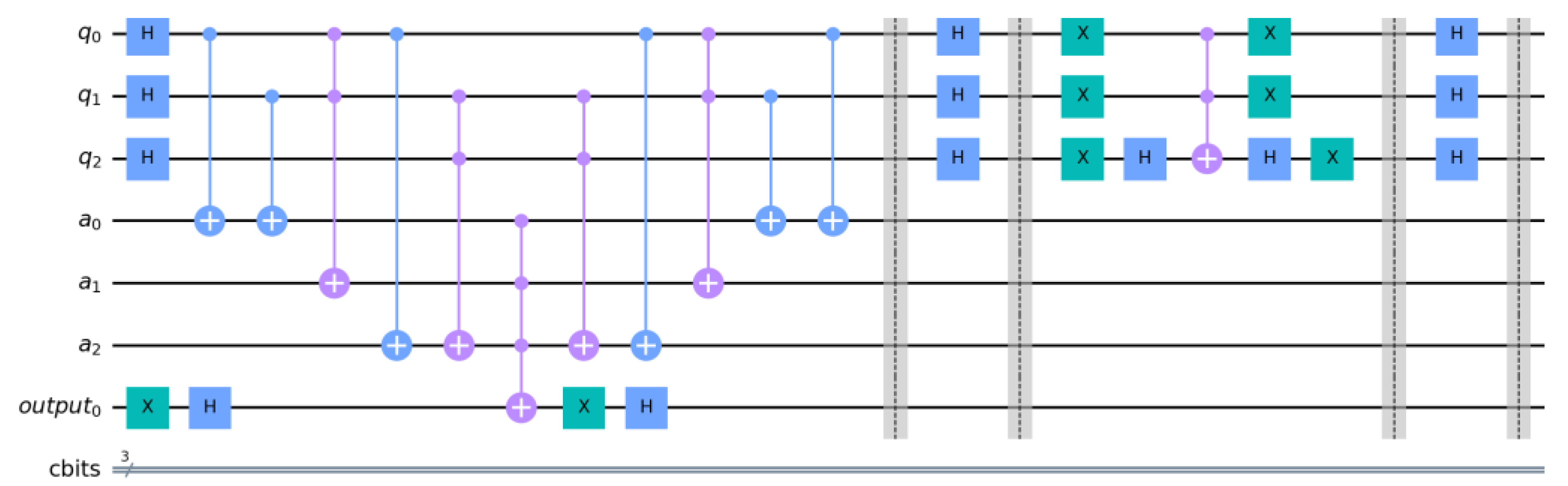
Figure 5 is a quantum circuit diagram of Equation (3).
The quantum circuit first used the XOR and AND elements to construct the oracle in the quantum circuit (the area before the first dashed line in
Figure 5) and introduced four ancilla bits to form the quantum circuit of the Boolean equations. Then, the phase of the quantum state was flipped by constructing the
operator (the region between the first and fourth dashed lines in
Figure 5), increasing the probability of the target state. Finally, the quantum state was measured using a measurement gate to obtain the target state. The quantum circuit could search for the correct answer with a probability close to 1 after one iteration of the quantum circuit.
4. Quantum Circuit Optimization
This paper focused on optimizing quantum circuits for solving Boolean equations to increase the solving scale. The main factors affecting the solving scale were the depth of the quantum circuit and the number of qubits. Reducing the depth of quantum circuits could be achieved with classical algorithm preprocessing. The quantum circuit for solving Boolean equations contained two kinds of qubits: the variable bits representing the variables of the equation and the ancilla bits representing the equation. With the increase in the solving scale of Boolean equations, ancilla bits accounted for more than 50% of all qubits, which significantly impacted the program’s execution. When building a quantum circuit, the variable bits could not be reduced, and the ancilla bits could be reduced by multiplexing the bits and using the phase quantum gate to replace the CX/CCX/MCX quantum gate.
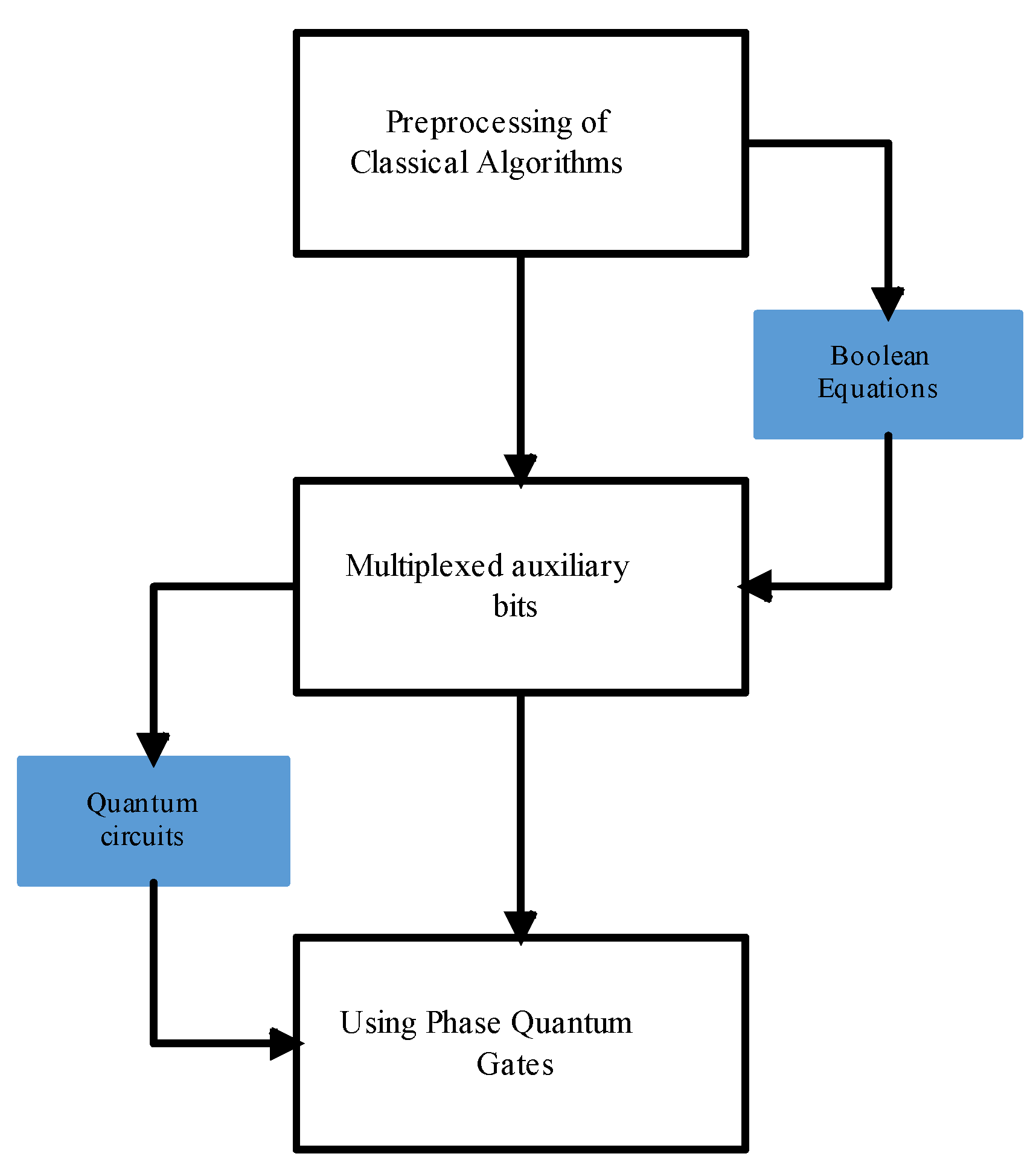
The quantum circuit optimization for solving Boolean equations included three steps: classical algorithm preprocessing, multiplexing the ancilla bits, and replacing CX/CCX/MCX quantum gates with phase quantum gates. The framework of the quantum circuit optimization process is shown in
Figure 6.
4.1. Preprocessing of Classical Algorithms
When the number of Boolean equation variables is too large, there are many identical terms in different equations in the equation system. According to the operation rules of Boolean equations, these identical terms can be eliminated from each other, thereby reducing the degree of complexity of Boolean equations. Equation (5) is a five-variable Boolean equation:
From Boolean Equation (5), it can be seen that Equation (3) (
) and Equation (4) (
) have the same terms, and the addition of these two equations can eliminate the terms to obtain a new equation (
). The degree of complexity of the new equation is less than those of Equations (3) and (4), so replacing Equation (3) or (4) with the new equation can simplify the Boolean equations without changing the solutions of the equations. This leads to the following general formula:
Adding Equation (6) to Equation (7) results in Equation (8):
Among them, a,b,c,..., z are discrete, increasing, random integers. If the number of terms of Equation (7) is less than the numbers of terms for Equations (5)–(7) can be added to the original Boolean equations to replace Equation (5) or (6) to optimize the degree of complexity of the Boolean equations.
4.2. Multiplexing Ancilla Bits
When the solving scale of Boolean equations reaches 14 variables, the total number of quantum qubits required is 29, of which the number of ancilla bits is 15, accounting for half of all the qubits. In building the quantum circuit for Boolean equation solving, an ancilla bit represents the state of an equation. The Boolean equations are grouped in an arithmetic-sequence-like method, and one ancilla bit can represent the states of multiple equations, which further reduces the number of ancilla bits and increases the solving scale. Formula (9) is used to find the minimum integer value of
t:
In (9),
s is the number of equations, and
t is the number of equations in the first group. On this basis, Algorithm 1 is used to find the grouping of Boolean equations.
| Algorithm 1. Find the grouping of Boolean equations. |
Require: g[100], T, i
Ensure: g[100] = {0}, T = 0, I = 0
1: while T ≤ s do
2: g[i] = t
3: T = T + t
4: i = i + 1
5: t = t − 1
6: end while
7: if T ≡ s then
8: return g[]
9: else T > s then
10: g[i] = (s + T)/2
11: return g[100]
12: end if |
The value stored in g[100] is the number of equations in each group.
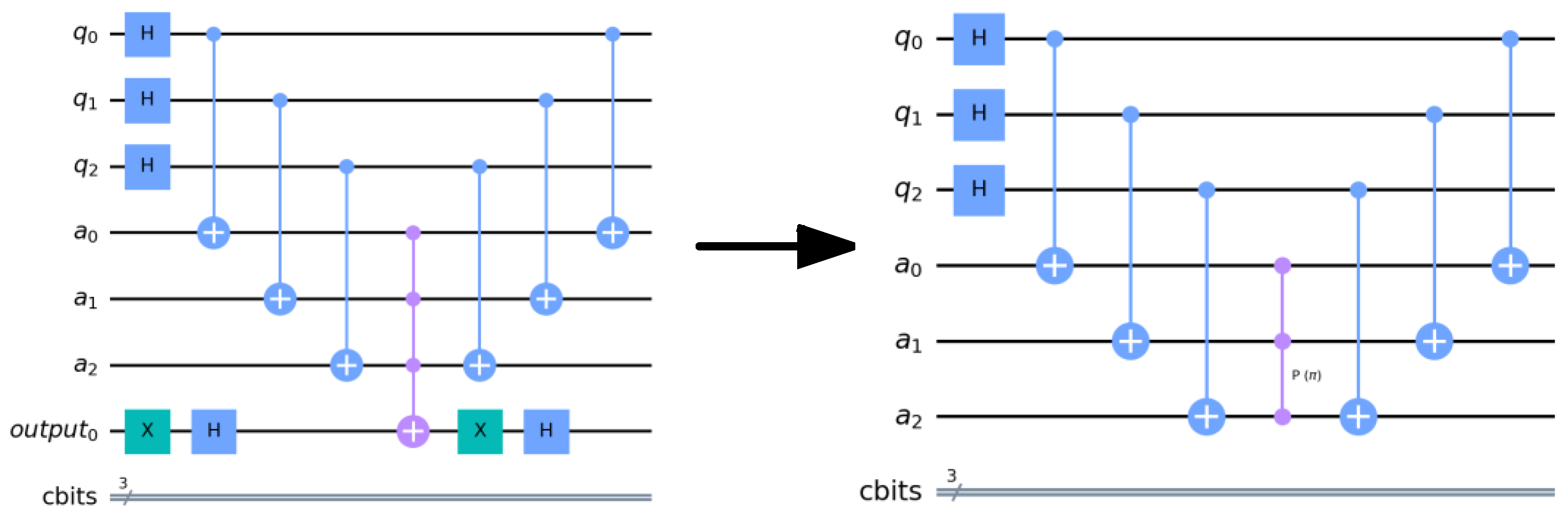
4.3. Using Phase Quantum Gates
According to the characteristics of the oracle in the Grover algorithm, the oracle marks the target state by inverting the phase of the quantum state [
6]. In the traditional Grover algorithm, the oracle is usually constructed using CX/CCX/MCX quantum gates, resulting in the need to use an additional ancilla bit. In theory, building an oracle with phase quantum gates can reduce one ancilla bit, as well as the depth of the quantum circuits, compared to CX/CCX/MCX gates, thereby increasing the rate and scale of solving Boolean equations. The replacement of CX/CCX/MCX quantum gates with phase quantum gates is shown in
Figure 7. We designed several sets of experiments to compare them and found that using phase quantum gates instead of CX/CCX/MCX gates could effectively improve the speed and scale of solving Boolean equations.
Through these methods, we successfully optimized the quantum circuit. The solution scale and speed of solving Boolean equations were improved. However, these optimization methods were limited to Boolean equations in a binary field. The multiplexing ancilla bit method dramatically reduced the number of qubits but deepened the depth of quantum circuits. Using the phase quantum gate method increased the solution scale to twenty-one variables, but it could not be solved stably for Boolean equations with too much complexity.
5. Experimental Results
In this paper, six experiments were carried out: classical algorithm preprocessing, multiplexing the ancilla bits, using phase quantum gates, etc. The experimental results showed that the maximum solving scale of the Boolean equations based on the Grover search algorithm could reach twenty-one variables.
The experiments were carried out with the Sugon cloud- computing cluster, and the experimental environment is shown in
Table 1. The dataset in the experiment was in two-dimensional array format, which contained the coefficients and values of the equations, from one variable to twenty-one variables. The code randomly generated the data and optimized to remove unqualified ones.
The first three experiments were classical algorithm preprocessing, multiplexing the ancilla bits, and using phase quantum gates.
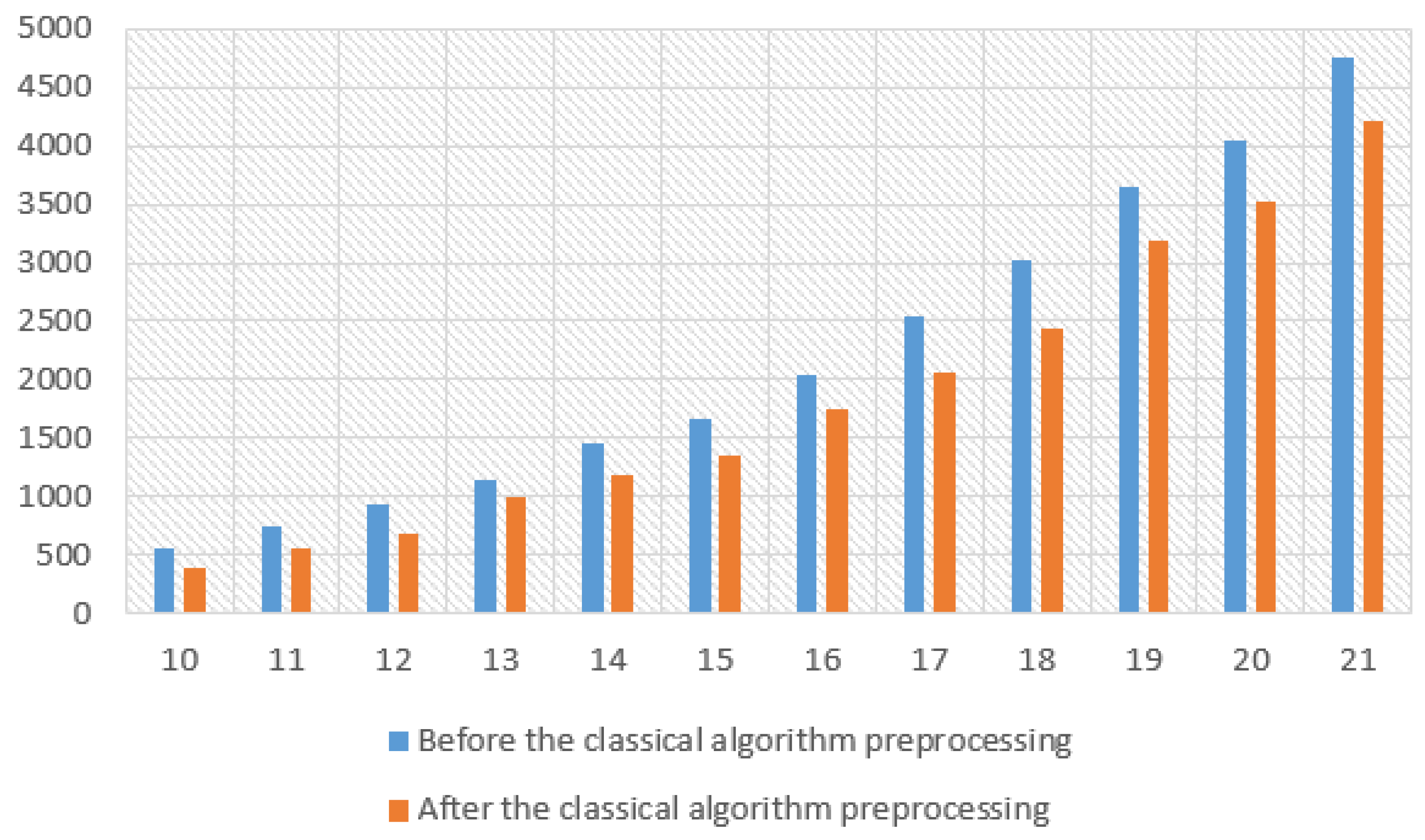
Figure 8 shows the changes in the number of Boolean equations before and after preprocessing with a classical algorithm (starting with 10 variables). The horizontal axis represented the number of variables in the Boolean equations, and the vertical axis represented the number of terms. As seen from the figure, the classical algorithm preprocessing eliminated the same terms in the equation, which could significantly reduce the degree of complexity of the Boolean equations in a relatively short time, which was helpful for the following solving operations of larger-scale Boolean equations.
Figure 9 shows the difference in the number of qubits before and after multiplexing the ancilla bits, where the horizontal axis represented the number of variables of the Boolean equations, and the vertical axis represented the number of qubits used by the quantum circuit. As seen from the figure, after the Boolean equations were grouped with the arithmetic sequence-like method, when the scale of the equation was small, the effect of multiplexing the ancilla bits was not obvious. However, with the increase in the solving scale of the equations, the number of quantum bits was significantly reduced, and the solving scale reached 19 variables.
Through the analysis of the oracle structure and experimental results, replacing the CX/CCX/MCX quantum gate with the phase quantum gate could achieve the same effect of marking the target state and reducing the number and depth of quantum circuits. As shown in
Figure 10, the targets of the quantum circuit in
Figure 7 were correctly marked. We compared the experimental results and found that, for a Boolean equation system with nineteen variables, the solution rate using the phase quantum gate was increased, and the solution scale was increased to twenty-one variables.
Next were three Boolean-equation-solving experiments. The first experiment was compared with the second to analyze the results and their probabilities for the two-variable and twenty-one-variable Boolean equations. The second one used two twenty-one-variable Boolean equations for comparison and analyzed the quantum circuit and the change in probability amplitude by iterating for different times. The third set of experiments analyzed the relationship between qubits and quantum circuits using multiple Boolean equations of varying scales.
Figure 11 shows the results of the Grover algorithm for solving two-variable Boolean equations. In this experiment, the answer was searched in a solution space of 2
2, the average quantum circuit depth was 34, and the shots were 1024. The correct answer could be found through only one G iteration, and the highest probability was obtained in all the cases.
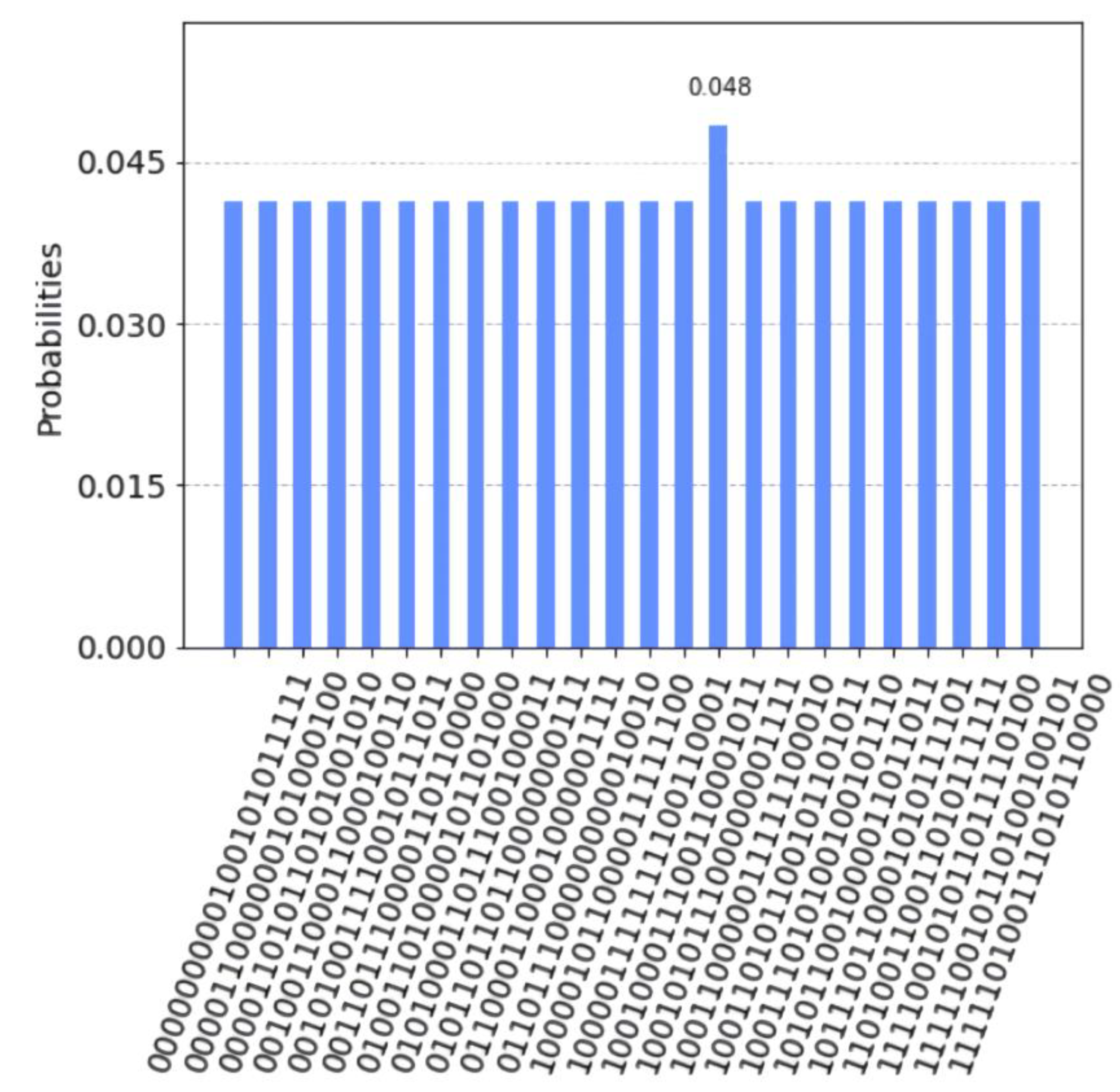
Figure 12 and
Figure 13 show the results of the Grover algorithm for solving Boolean equations with twenty-one variables in a solution space of 2
21 with one and three iterations, respectively. The shots were one million, and the respective average quantum circuit depths were 67,897 and 229,503 (because there was too much data in the solution space, only part of the data was selected for display). It can be seen from the experimental results that the algorithm did not obtain the correct answer when iterated one time and obtained the answer with a higher probability—100101011100000001111—when iterating three times. Through the relationship between the probability amplitude, the number of iterations, and the depth of the quantum circuit, we know that, when the number of iterations increased, the probability of the Grover algorithm successfully finding the target increased. However, the quantum circuit was also deeper, which affected the solving scale and time. In this experiment, the algorithm performed three G iterations to search for the correct answer in the vast solution space with a high probability, and when iterated
times, the algorithm searched for the answer with a probability close to 1.
To fully understand the relationship between the number of qubits and quantum circuits, Qiskit was used to solve Boolean equations on different scales many times, and the experimental results were recorded.
Table 2 lists the number of qubits and the average quantum circuit depth (three iterations) used for Boolean equations on different scales (starting with ten variables).
It can be seen from
Table 2 that, when the scale of the Boolean equations increased, the depth of the quantum circuit became increasingly deeper with the increase in the number of qubits and the number of iterations. When the solving scale reached 22 variables, because the quantum circuit was too deep and the number of qubits was too large, the simulator in Qiskit could not continue to run. Through these three experiments, the situation of the Grover search algorithm for solving large-scale Boolean equations was fully demonstrated.
6. Conclusions
Quantum computing is a rapidly emerging technology that follows the laws of quantum mechanics and uses qubits for computing. Compared with classical computers, quantum computers have obvious advantages in many aspects, such as accuracy and efficiency. Quantum algorithms can perform any computation exponentially more efficiently on quantum computers than on conventional computers.
In this paper, we used the quantum simulator provided by the Qiskit framework to run the Grover algorithm to solve nonlinear Boolean equations in a binary field and prove the feasibility of the Grover algorithm on this problem. By analyzing the structure of Boolean equations and quantum circuits, the quantum circuits were optimized, increasing the solving scale to twenty-one variables. When building a quantum circuit, using classical algorithm preprocessing, multiplexing the ancilla bits, and phase quantum gates to optimize the quantum circuit while increasing the solving scale of Boolean equations, the depth of the quantum circuit was significantly deepened. The experiments showed that the depth of the quantum circuit had a significant influence on the solution of Boolean equations. In theory, if the depth of the quantum circuit could be reduced, the solving scale could continue to grow. When using the Grover algorithm to solve Boolean equations, the main factor affecting the solving scale was the oracle, making the quantum circuit depth rise when distinguishing the target. It was affected by noise when searching for a target, which seriously reduced the probability amplitude of the target.
Our current work mainly was to verify the feasibility of the Grover algorithm in solving Boolean equations and to conduct preliminary experiments to explore the full scale of solving Boolean equations. In future work, we plan to study two aspects: (1) simplifying the terms of Boolean equations using data structures that store the equations efficiently and (2) continuing to optimize the quantum circuit and reduce the impact of noise on the target through oracle optimization.


