
Defect Detection Scheme for Key Equipment of Transmission Line for Complex Environment

Abstract
:1. Introduction
- This paper uses a more lightweight network. The feature extraction network VGG-16 of Faster R-CNN is replaced by a lightweight MobileNet network, which greatly reduces redundant computation.
- In this paper, the soft-NMS algorithm is used to replace the original NMS algorithm to improve the detection accuracy, and CAROI is used to replace the original ROI pooling layer to maintain the original structure of small-sized components to improve the detection accuracy.
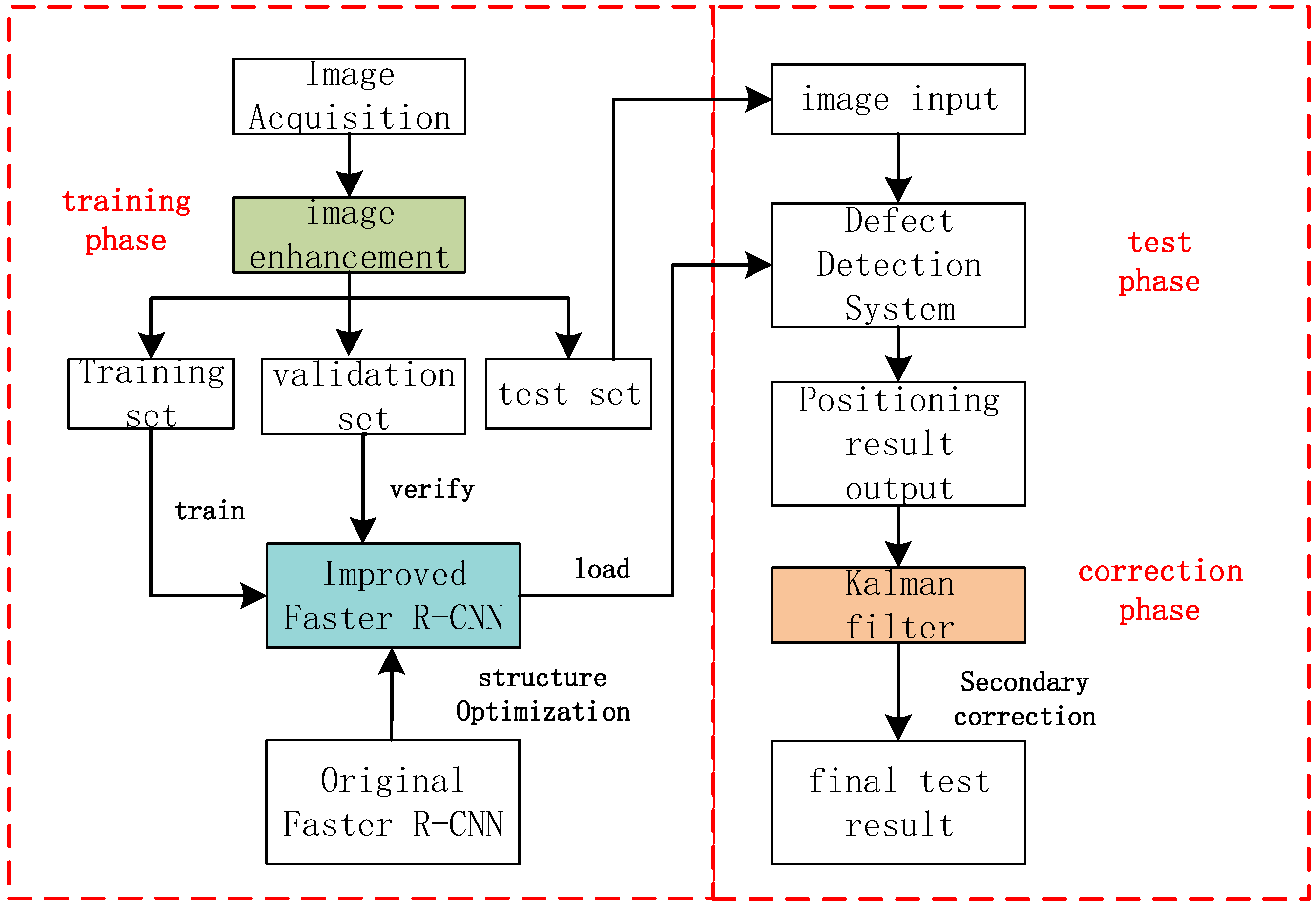
2. System Overview
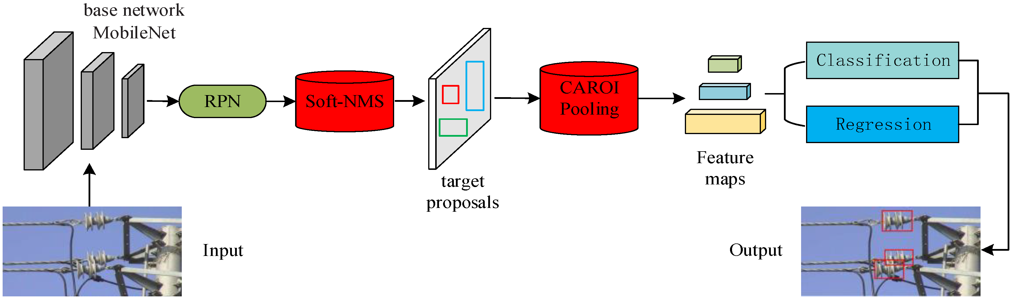
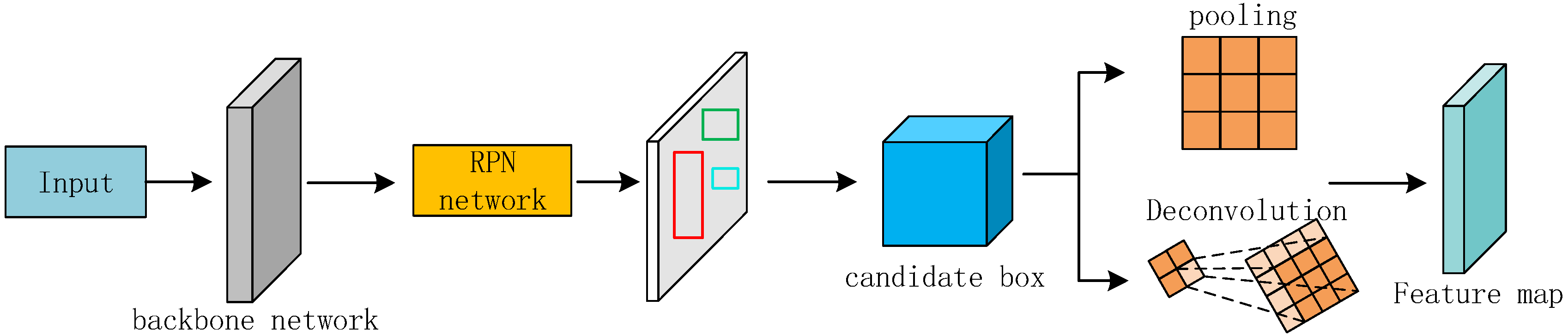
3. Faster R-CNN Framework Improvement
3.1. Basic Network
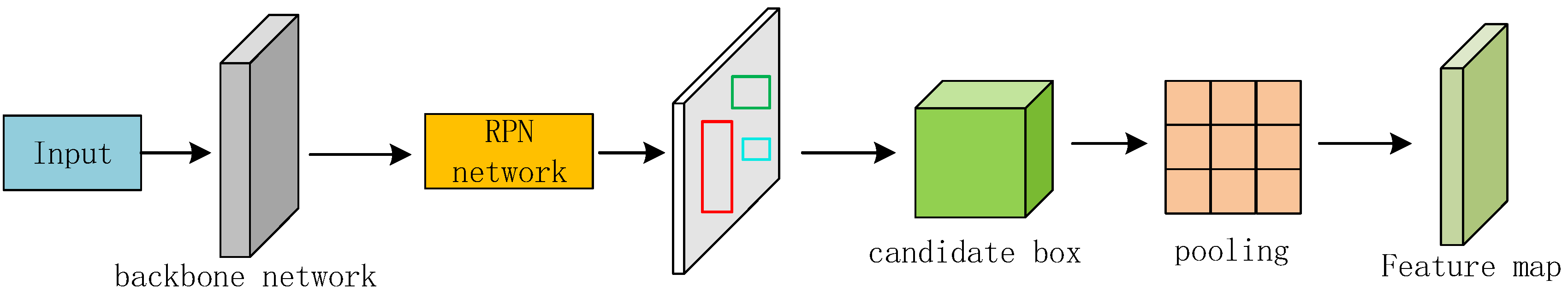
3.2. RPN Network
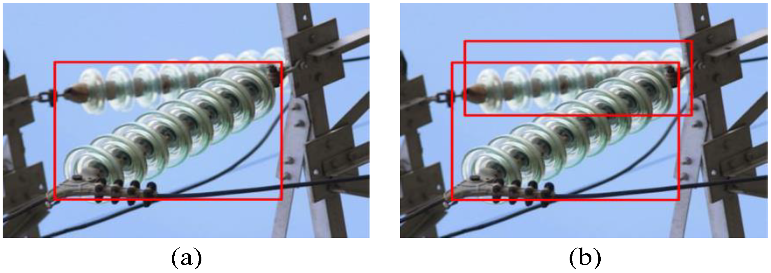
3.3. Context-Aware ROI Pooling
4. Kalman Filter Correction
5. Experimental Results and Analysis
5.1. Experimental Environment
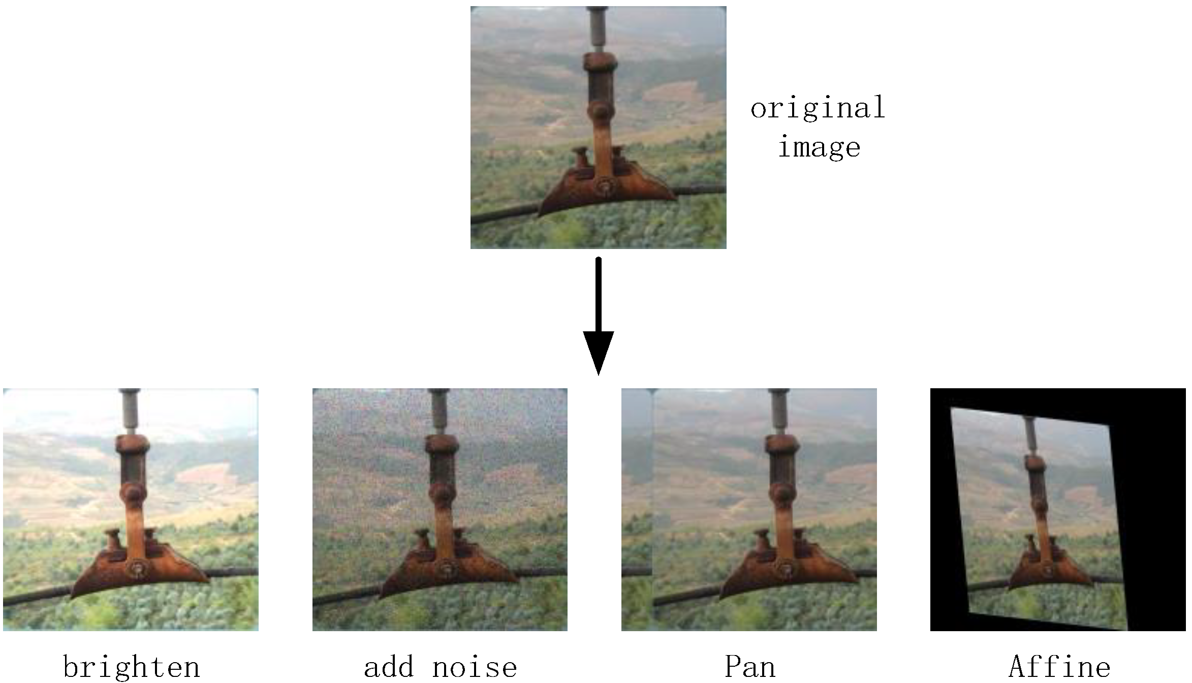
5.2. Dataset Processing
5.3. Model Training Parameter Settings
5.4. Evaluation Indicators
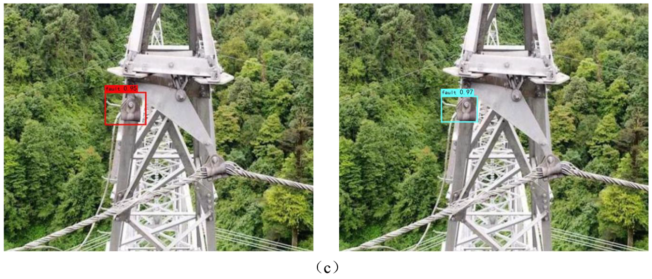
5.5. Display of Experimental Results
5.6. Comparison and Analysis of Experimental Results of Different Algorithms
6. Conclusions
Author Contributions
Funding
Conflicts of Interest
References
- Liu, H. National Quality Infrastructure Supports Smart Grid Construction in China-Taking the State Grid as an Example. IOP Conf. Ser. Earth Environ. Sci. 2020, 531, 012011. [Google Scholar] [CrossRef]
- Devices Create Smarter Grids with Accurate Line Fault Detection; Transmission & Distribution World: Overland Park, KS, USA, 2019.
- Wang, S.; Zhou, Z.; Zhao, W. Semantic Segmentation and Defect Detection of Aerial Insulators of Transmission Lines. J. Phys. Conf. Ser. 2022, 2185, 012086. [Google Scholar] [CrossRef]
- Li, Y.; Song, Y.; Yang, Z.; Xie, X. Use of line laser scanning thermography for the defect detection and evaluation of composite material. Sci. Eng. Compos. Mater. 2022, 29, 74–83. [Google Scholar] [CrossRef]
- Yücel, M.K.; Legg, M.; Kappatos, V.; Gan, T.-H. An ultrasonic guided wave approach for the inspection of overhead transmission line cables. Appl. Acoust. 2017, 122, 23–34. [Google Scholar] [CrossRef]
- Zhang, Q.; Chang, X.; Meng, Z.; Li, Y. Equipment detection and recognition in electric power room based on faster R-CNN. Procedia Comput. Sci. 2021, 183, 324–330. [Google Scholar] [CrossRef]
- Liu, X.; Lin, Y.; Jiang, H.; Miao, X.; Chen, J. Slippage fault diagnosis of dampers for transmission lines based on faster R-CNN and distance constraint. Electr. Power Syst. Res. 2021, 199, 107449. [Google Scholar] [CrossRef]
- Rodriguez, F.M., Jr.; Bastos, G.B.; Seruffo, M.C.R.; Costa, F.A.R.; Figueiredo, K.; de Melo, H., Jr. Analysis of migration to the Brazilian free energy market based on statistical methods and artificial neural networks. SBIC 2021, 1–8. [Google Scholar] [CrossRef]
- Zhou, J.H.; Liu, Z.Y.; Chen, G. Intelligent Inspection of the High-Speed Train Bogie Flaw Based on Eddy Current. Appl. Mech. Mater. 2015, 3785, 738–739. [Google Scholar] [CrossRef]
- Huang, H.; Huang, Y.; Mu, X.; Wang, X. Research on Recognition and Location Method of Insulator in Infrared Image Based on Deep Learning. J. Phys. Conf. Ser. 2021, 2087, 012090. [Google Scholar] [CrossRef]
- Wang, W.; Wei, J.; Zhu, Y.; Zhou, S. Power distribution equipment and defect identification technology based on deep learning. J. Phys. Conf. Ser. 2021, 2030, 012075. [Google Scholar] [CrossRef]
- Tao, W.; Wang, W.; Yue, L.; Xie, B.; Yin, W.; Wang, H. Insulator Defect Detection Method for Lightweight YOLOV3. Comput. Eng. 2019, 45, 275–280. [Google Scholar]
- Alahyari, A.; Hinneck, A.; Tariverdi, R.; Pozo, D. Segmentation and Defect Classification of the Power Line Insulators: A Deep Learning-based Approach. arXiv 2020, arXiv:2009.10163. [Google Scholar]
- Lan, Y.; Xu, W. Insulator defect detection algorithm based on a lightweight network. J. Phys. Conf. Ser. 2022, 2181, 012007. [Google Scholar] [CrossRef]
- Qi, Y.; Du, L.; Zhao, Z.; Cui, Y.; Si, W. Insulator Detection Based on SSD with the Default Box Adaptively Selection. Comput. Sci. Appl. Eng. 2018, 110, 1–4. [Google Scholar] [CrossRef]
- Ni, H.; Wang, M.; Zhao, L. An improved Faster R-CNN for defect recognition of key components of transmission line. Math. Biosci. Eng. 2021, 18, 4679–4695. [Google Scholar] [CrossRef]
- Zhao, Z.; Fan, X.; Xu, G.; Zhang, L.; Qi, Y.; Zhang, K. Aggregating Deep Convolutional Feature Maps for Insulator Detection in Infrared Images. IEEE Access 2017, 5, 21831–21839. [Google Scholar] [CrossRef]
- Zhou, Y.; Wen, S.; Wang, D.; Mu, J.; Irampaye, R. Object Detection in Autonomous Driving Scenarios Based on an Improved Faster-RCNN. Appl. Sci. 2021, 11, 11630. [Google Scholar] [CrossRef]
- Lv, L.; Tan, Y. Detection of cabinet in equipment floor based on AlexNet and SSD model. J. Eng. 2019, 2019, 605–608. [Google Scholar] [CrossRef]
- Gao, S.; Kang, G.; Yu, L.; Zhang, D.; Wei, X.; Zhan, D. Adaptive Deep Learning for High-Speed Railway Catenary Swivel Clevis Defects Detection. IEEE Trans. Intell. Transp. Syst. 2020, 23, 1299–1310. [Google Scholar] [CrossRef]
- Zhu, J.; Chang, X.; Zhang, X.; Su, Y.; Long, X. A Novel Method for the Reconstruction of Road Profiles from Measured Vehicle Responses Based on the Kalman Filter Method. Comput. Model. Eng. Sci. 2022, 130, 1719–1735. [Google Scholar] [CrossRef]
- Ren, K.; Zhang, D.; Mohammed, S.; Calvi, A. A Kalman filtering fuzzy logic algorithm for recognition of lane departure. J. Intell. Fuzzy Syst. 2021, 41, 4855–4862. [Google Scholar] [CrossRef]
- Liu, Z.; Liu, W.; Han, Z. A high-precision detection approach for catenary geometry parameters of electrical railway. IEEE Trans. Instrum. Meas. 2017, 66, 1798–1808. [Google Scholar] [CrossRef]
- Li, Y.; Huang, H.; Xie, Q.; Yao, L.; Chen, Q. Research on a Surface Defect Detection Algorithm Based on MobileNet-SSD. Appl. Sci. 2018, 8, 1678. [Google Scholar] [CrossRef] [Green Version]
- Bodla, N.; Singh, B.; Chellappa, R.; Davis, L.S. Soft-NMS—Improving Object Detection with One Line of Code. In Proceedings of the 2017 IEEE International Conference on Computer Vision (ICCV), Venice, Italy, 22–29 October 2017. [Google Scholar]
- Yao, L.; Sheng, Q.Z.; Qin, Y.; Wang, X.; Shemshadi, A.; He, Q. Context-aware Point-of-Interest Recommendation Using Tensor Factorization with Social Regularization. In Proceedings of the International ACM Sigir Conference, Santiago, Chile, 9–13 August 2015; ACM: New York, NY, USA, 2015. [Google Scholar]
- Xie, X.; Xiao, H.; Quan, L.; Shi, G. Visualization and Pruning of SSD with the base network VGG16. In Proceedings of the 2017 International Conference, Paris, France, 21–25 May 2017; ACM: New York, NY, USA, 2017. [Google Scholar]
- Shi, M.; Ouyang, P.; Yin, S.; Liu, L.; Wei, S. A Fast and Power-Efficient Hardware Architecture for Non-Maximum Suppression. IEEE Trans. Circuits Syst. II Express Briefs 2019, 66, 1870–1874. [Google Scholar] [CrossRef]
- Wang, Y.; Liu, Z.; Deng, W. Anchor Generation Optimization and Region of Interest Assignment for Vehicle Detection. Sensors 2019, 19, 1089. [Google Scholar] [CrossRef] [PubMed] [Green Version]
- Tun, N.L.; Gavrilov, A.; Tun, N.M.; Trieu, D.M.; Aung, H. Remote Sensing Data Classification Using a Hybrid Pre-Trained VGG16 CNN-SVM Classifier. In Proceedings of the 2021 IEEE Conference of Russian Young Researchers in Electrical and Electronic Engineering (ElConRus), Moscow, Russia, 26–29 January 2021. [Google Scholar]
- Zhao, W.; Yan, H.; Shao, X. Object detection based on improved non-maximum suppression algorithm. Appl. Soft Comput. 2019, 81, 105478. [Google Scholar]
- Wang, K.; Liu, M.Z. Object Recognition at Night Scene Based on DCGAN and Faster R-CNN. IEEE Access 2020, 8, 193168–193182. [Google Scholar] [CrossRef]
- Yan, C.; Chen, W.; Chen, P.C.Y.; Kendrick, A.S.; Wu, X. A new two-stage object detection network without RoI-Pooling. In Proceedings of the 2018 Chinese Control and Decision Conference (CCDC), Shenyang, China, 9–11 June 2018. [Google Scholar]
- Hu, X.; Xu, X.; Xiao, Y.; Chen, H. SINet: A Scale-insensitive Convolutional Neural Network for Fast Vehicle Detection. IEEE Trans. Intell. Transp. Syst. 2018, 3, 1–10. [Google Scholar] [CrossRef] [Green Version]
- Luisier, F.; Blu, T.; Unser, M. Image Denoising in Mixed Poisson–Gaussian Noise. IEEE Trans. Image Process. 2011, 20, 696–708. [Google Scholar] [CrossRef] [Green Version]
- Sun, K.; Simon, S. Bilateral Spectrum Weighted Total Variation for Real-World Super-Resolution and Image Denoising. arXiv 2021, arXiv:2106.00768. [Google Scholar]
- Foi, A.; Trimeche, M.; Katkovnik, V.; Egiazarian, K. Practical Poissonian-Gaussian Noise Modeling and Fitting for Single-Image Raw-Data. IEEE Trans. Image Process. 2008, 17, 1737–1754. [Google Scholar] [CrossRef] [Green Version]
- An, Y.; Wang, X.; Chu, R.; Yue, B.; Wu, L.; Cui, J.; Qu, Z. Event classification for natural gas pipeline safety monitoring based on long short-term memory network and Adam algorithm. Struct. Health Monit. 2019, 19, 1151–1159. [Google Scholar] [CrossRef]
- Fraser, C.T.; Ulrich, S. Adaptive extended Kalman filtering strategies for spacecraft formation relative navigation. Acta Astronaut. 2021, 178, 700–721. [Google Scholar] [CrossRef]
- Zhang, Y.; Wang, R.; Li, S.; Qi, S. Temperature Sensor Denoising Algorithm Based on Curve Fitting and Compound Kalman Filtering. Sensors 2020, 20, 1959. [Google Scholar] [CrossRef] [PubMed] [Green Version]
- Kohli, H.; Agarwal, J.; Kumar, M. An Improved Method for Text Detection using Adam Optimization Algorithm. Glob. Transit. Proc. 2022, 3, 230–234. [Google Scholar] [CrossRef]


| Model | Precision (%) | Madd (Million) | Parameter (Million) |
|---|---|---|---|
| VGG-16 | 71.52 | 16,000 | 140 |
| MobileNet | 70.83 | 570 | 4.3 |
| Category | Version |
|---|---|
| operating system | Windows 10 |
| CPU | Intel Core i9-10900 k |
| GPU | NVIDIA GeForce GTX 3080 |
| RAM | 32 GB |
| Tensorflow-gpu | Tensorflow-gpu1.13.2 |
| Keras | Keras2.1.5 |
| Cuda | Cuda10.0 |
| Cudnn | Cudnn7.4.1.5 |
| Defet Detection Methods | P (%) | R (%) | mAP (%) | IOU (%) | Detection Time (s) |
|---|---|---|---|---|---|
| YOLO | 61.23 | 59.61 | 60.61 | 60.24 | 0.04 |
| SSD | 77.96 | 73.18 | 77.42 | 76.55 | 0.06 |
| MS-CNN | 85.83 | 83.06 | 86.53 | 83.36 | 0.40 |
| Original Faster R-CNN | 80.36 | 78.62 | 80.05 | 80.16 | 2.00 |
| Improve Faster R-CNN | 86.44 | 83.09 | 86.16 | 85.31 | 0.10 |
| Improve Faster R-CNN + Kalman filter | 90.26 | 87.49 | 91.10 | 88.37 | 0.12 |
| Number of Defective Samples | /% | |||||
|---|---|---|---|---|---|---|
| 1 | 5 | 10 | 20 | 30 | 40 | |
| 10 | 82.35 | 81.25 | 79.58 | 76.35 | 74.35 | 72.14 |
| 20 | 83.25 | 82.42 | 82.32 | 81.35 | 79.56 | 78.36 |
| 50 | 85.65 | 84.54 | 83.35 | 83.14 | 82.54 | 78.25 |
| Denoising Methods | P (%) | R (%) | mAP (%) | IOU (%) | Detection Time (s) |
|---|---|---|---|---|---|
| mean filter | 86.25 | 87.26 | 84.58 | 88.65 | 0.14 |
| median filter | 85.32 | 83.54 | 86.76 | 85.47 | 0.11 |
| wavelet denoising | 84.35 | 85.25 | 87.54 | 84.35 | 0.13 |
| Gaussian filter | 80.32 | 79.61 | 78.65 | 81.23 | 0.09 |
| bilateral filter | 87.35 | 85.36 | 88.45 | 84.36 | 0.13 |
| Kalman filter | 90.26 | 87.49 | 91.10 | 88.37 | 0.12 |
Publisher’s Note: MDPI stays neutral with regard to jurisdictional claims in published maps and institutional affiliations. |
© 2022 by the authors. Licensee MDPI, Basel, Switzerland. This article is an open access article distributed under the terms and conditions of the Creative Commons Attribution (CC BY) license (https://creativecommons.org/licenses/by/4.0/).
Share and Cite
Wang, J.; Deng, F.; Wei, B. Defect Detection Scheme for Key Equipment of Transmission Line for Complex Environment. Electronics 2022, 11, 2332. https://doi.org/10.3390/electronics11152332
Wang J, Deng F, Wei B. Defect Detection Scheme for Key Equipment of Transmission Line for Complex Environment. Electronics. 2022; 11(15):2332. https://doi.org/10.3390/electronics11152332
Chicago/Turabian StyleWang, Jian, Fangming Deng, and Baoquan Wei. 2022. "Defect Detection Scheme for Key Equipment of Transmission Line for Complex Environment" Electronics 11, no. 15: 2332. https://doi.org/10.3390/electronics11152332