Combination of Optimized Variational Mode Decomposition and Deep Transfer Learning: A Better Fault Diagnosis Approach for Diesel Engines

Abstract

Extracting features manually and employing preeminent knowledge is overly utilized in methods to conduct fault diagnosis. A diagnosis approach utilizing intelligent methods of the optimized variational mode decomposition and deep transfer learning is proposed in this manuscript to deal with fault diagnosis. Firstly, the variational mode decomposition is optimized by K values of the dispersion entropy to realize an adaptive decomposition and reduce the noise of the signal. Secondly, an image with two dimensions is generated by a vibration signal with one dimension utilizing a short-time Fourier transform, after conducting noise reduction. Then, the ResNet18 network model is used to pre-train the model. Finally, the model transfer method is used to detect faults of a diesel engine. The results show that the proposed method outperforms the deep learning methods available in the literature. Besides, better noise reduction ability and higher diagnostic accuracy are attained.

1. Introduction

Diesel engines are generally utilized in the construction of machinery, automobiles, vessels, and in other production areas. Due to their complex design structure and their long-term operation in harsh environments, various failures will inevitably occur, which lead to prolonged equipment downtime and increased maintenance costs. So, dealing with these issues has become a hot research direction, contemporarily studied by many scholars. Moreover, various intelligent data-driven approaches to coping with fault diagnosis of diesel engine failures have been suggested and satisfactory research outcomes have been achieved [1,2,3].

Fault diagnosis approaches with machine learning methodologies substantially include three fault facets: extraction of features, reduction of feature dimensionality, and pattern recognition of features. For these purposes, the time-frequency analysis of the vibration signal is studied, the commonly implemented algorithms of which are called Hilbert Huang Transform (HHT), Wavelet Transform (WT), and Short Time Fourier Transform (STFT) [4,5,6]. The implementations of these algorithms aim at extracting the feature parameters of both time and frequency domains [7,8]. When feature dimensionality reduction is under consideration, principal component analysis (PCA), kernel principal component analysis (k-PCA), and autoencoder are generally implemented [9,10,11]. Similarly, when pattern recognition is under consideration, support vector machine (SVM), random forest (RF), and k-nearest neighbor (k-NN) methods are commonly utilized [12,13,14]. Thus, these feature extraction and dimensionality reduction techniques are combined to detect pattern recognition of various failures. Moreover, various diagnostic methods to detect faults in diesel engines have been suggested [15,16,17].

The conventional diagnosis methods utilizing intelligent approaches constitute a small set of machine learning methods with higher diagnosis accuracies. However, they are also accompanied by restrictions, as follows:

(1) Due to a large quantity of both noise and interference available in sampled vibration signals, detection of weak fault signals is generally difficult. To cope with weak fault signals, more advanced signal preprocessing techniques must be employed [18].

(2) If the feature parameters are set improperly, or rely on largely preeminent knowledge of experts [19,20], the accuracy of fault diagnosis is affected.

As artificial intelligence technology rapidly advances, deep learning has gradually turned into an efficient method and surmounts the deficiencies of the conventional fault diagnosis approaches. So, extracting useful fault features directly from raw data is a key advantage. Hence, deep belief network (DBN), convolutional neural network (CNN), and long short-term memory network (LSMN) are commonly implemented to diagnose faults related to mechanical applications [21,22]. The DBN was implemented by Xu et al. [23] to diagnose the air path fault of turbofan engines with higher classification accuracy. The parameters of the CNN were optimized by Zhou et al. [24], by utilizing the sorting method of input measurement parameters, which was applied to detect the fault of the gas circuit of an engine with a relatively ideal diagnosis impact. Han et al. [25] constructed a data-driven fault prediction model using an LSTM network and applied it to marine diesel engines, and obtained better fault prediction results.

Theproblems expressed below still exist and need to be dealt with:

(1) Since diesel engines work in complex environments for a long time, weak fault features are masked by stronger noise and interference signals, which greatly increases the difficulty of direct fault diagnosis using one-dimensional vibration signals.

(2) The parameters in network training increase with the increment of the number of hidden layers. When a multi-layer deep network model is trained, both preparing labeled samples in large quantities and the requirements of computational power and time need to be taken into account. However, collecting a large amount of data with faulty tags is almost impossible when the equipment basically runs in a steady state, in which few failures could occur.

When training a multi-layer deep network model from scratch, there is not only a need to prepare a large number of labeled samples, but also the training consumes a lot of computing power and time. Then, in practical engineering applications, the equipment is running in a normal condition, and there exist few failures, which makes it impossible to obtain a large number of data samples with faulty tags.

(3) The hyperparameter optimization and selection of the deep learning network model consumes a lot of time in training the network model and, thus, this will directly affect its performance.

Due to the issues mentioned above, a method called transfer learning (TL) was suggested when mechanical fault diagnosis is under consideration. Xu et al. [26] suggested an approach employing migration component analysis to determine fault diagnosis when various working conditions were taken into account. Zhao et al. [27] realized cross-domain aero-engine fault diagnosis by employing extreme learning machines, using the TL method. Xiong et al. [28] suggested a methodology utilizing stacked autoencoders and feature transfer to diagnose diesel engine faults. Both training and optimizing the deep learning network model are essential when the available TL research is under consideration, which restricts its application in engineering implementations.

To resolve the issues presented above, this manuscript suggests a methodology to diagnose faults utilizing both optimized variational mode decomposition (VMD) and deep transfer learning (DTL), concurrently. Firstly, the VMD method is optimized by using the K value of the dispersion entropy to conduct the noise reduction in the original vibration. Then, the noise-reduced vibration signal is converted into a frequency map with two dimensions by the STFT method. To lower both training time and computational complexity of the deep learning network model, a TL method, based on the ResNet18 network model, is suggested, which could effectively extract useful features from the frequency map represented by two dimensions, and quickly achieve accurate fault classification. Finally, experiments conducted present both better-extracted features and higher diagnostic accuracies.

The key contributions of the manuscript are expressed as follows:

(1) The optimized VMD can not only withhold weak fault signals, but also better excludes both noisy and interfering signals in the original vibration signal, which results in successful noise reduction.

(2) By employing the ResNet18 network model, trained on the ImageNet dataset as the transfer object, which provides a fine-tuning of the network structure, the training time of the network could be effectively lowered, and the accuracy of identifying faults could be improved.

(3) This research utilizes both optimized VMD and DTL concurrently to extract and classify fault features of diesel engines in strong noise environments. The proposed method exhibited greatly improved performance and a practically usable form to diagnose faults in applications in experiments.

The remaining sections of the manuscript are constructed as follows: A method dealing with noise reduction utilizing the optimized VMD is described in Section 2. Section 3 details the basic theory of time-frequency images and DTL models. The fault diagnosis process of a diesel engine, utilizing both optimized VMD and DTL, is described in Section 4. Section 5 analyzes and validates the method suggested in this manuscript employing pre-set experiments. The conclusion is provided in Section 6. Abbreviations provides the commonly used symbols in this manuscript.

2. A Noise Reduction Approach Utilizing the Optimal VMD

The VMD, Variational Mode Decomposition, as a novel non-stationary and non-linear signal processing methodology, was proposed in [29]. By resolving the constrained variational problem to replace the previous empirical mode decomposition (EMD), ensemble empirical mode decomposition (EEMD), and local mean decomposition (LMD) were suggested [30]. Hence, the modal aliasing and end effect problems of the conventional decomposition method were improved. However, the VMD itself also has certain limitations. The determination of its decomposition level K needs to be set manually, which has a certain degree of subjectivity and randomness that will have an impact on the modal decomposition process. Therefore, this paper adopts a method of optimizing the VMD based on the K value of dispersion entropy to realize the adaptive decomposition and reconstruction of noise reduction of the signal.

2.1. The VMD

The function of the VMD is to establish and resolve the variational problem, and decompose the available signal f into K Intrinsic Mode Function (IMF) components, $u_k(t)$. Both epicenter frequency and bandwidth are continuously revised by running the process iteratively, since the summation of each component is assumed to be equal to the input signal. Then, the IMF component minimizing the summation of the bandwidths related to the IMF is obtained, as follows:

(1) By running the Hilbert transform, the $u_k(t) (k=1,2,\cdot \cdot \cdot ,K)$ analytic signal unilateral spectrum of each IMF component is obtained, namely,

$$[\delta (t)+(j/\pi t)]\times u_k(t)$$

(1)

then, the position of the center frequency of each eigenmode to the corresponding baseband is expressed by

$$\left\{[\delta (t)+(j/\pi t)]\times u_k(t)\right\}{e}^{-j{\omega }_{k}t}$$

(2)

where the impulse function is denoted by $\delta (t)$, the sign “$\ast$” represents the convolution calculation, and ${\omega }_k$ represents the center frequency of each IMF component;

(2) The L² norm of the gradient of the demodulated signal is computed, and the bandwidth of each IMF component is estimated. Then, the constrained variational model expression is expressed by

$$\left\{\begin{array}{c}\underset{\{u_k,{\omega }_k\}}{\min }\left\{{\displaystyle \sum _{k=1}^K{\Vert {\partial }_t\left[(\delta (t)+\frac{j}{\pi t})\times u_k(t)\right]e^{-j{\omega }_{k}t}\Vert }_2^2}\right\}\\ s.t{\displaystyle \sum _{k=1}^K{u}_k=f(t)}\end{array}\right\}$$

(3)

where n ${\Vert \Vert }_2$ denotes the L² norm operation; $u_k=\left\{u_1,u_2,\cdots ,u_k\right\}$ is the k IMF component, and $f(t)$ represents the original time-domain signal; ${\omega }_k=\left\{{\omega }_1,{\omega }_2,\cdots ,{\omega }_k\right\}$ represents the central frequency of each component

(3) Both α and λ are used in the solution of the variational problem, which is called the quadratic penalty factor and the Lagrange multiplication operator. Then, the constrained variational problem is transformed into an unconstrained form, in which the Lagrange function in the augmented form is expressed by

$$\begin{array}{ll}L(\{u_k\},\{{\omega }_k\},\lambda )=& \alpha {{\displaystyle \sum _k\Vert {\partial }_t\left[(\delta (t)+\frac{j}{\pi t})\times u_k(t)\right]e^{-j{w}_{k}t}\Vert }}_2^2\hfill \\ & +{\Vert f(t)-{\displaystyle \sum _{k=1}^K{u}_k(t)}\Vert }_2^2\\ & +(\lambda (t),f(t)-{\displaystyle \sum _{k=1}^K{u}_k(t)})\end{array}$$

(4)

where α represents the quadratic penalty factor, which is usually selected as a positive large number to enhance the accuracy of the reconstructed signal; λ is called the Lagrange multiplication operator, and λ(t) guarantees strict constraints. ADMM, the Alternate Direction Method of Multipliers, is employed to recompute the values u_k, ω_k and λ in each component. Then, the saddle point of the augmented Lagrange function is calculated, namely, the constrained variational model is optimized to realize modal decomposition.

2.2. Dispersion Entropy

The principle of the VMD signal decomposition was introduced in the previous section. However, determining the VMD decomposition layers, K, needs to be set manually. So, K would directly have an impact on the decomposition effect of the signal when a complex signal is processed. When K is set to large numbers, over-decomposition could occur, thus redundant components would be obtained. On the other hand, when K is assigned to small numbers, under-decomposition could happen and, thus, the useful signal could not be effectively separated. In this paper, it is proposed that K is optimized by employing scatter entropy to find and conduct the decomposition of the signal adaptively.

DE, Dispersion Entropy, is a novel method suggested by Rostaghi and Azami in 2016 to measure the complexity of time series [31]. The fact that conventional permutation entropy does not consider the magnitude of amplitude was remedied and, thus, better stability and faster calculation were mentioned as advantages. The steps are presented by:

(1) The function of the normal distribution is selected as the nonlinear normalization function. The sequence x = {x₁, x₂, …, x_N} is normalized with the mean and standard deviation of x as parameters. Then y = {y₁, y₂, …, y_N} is attained, where N represents the sequence length with y ∈ (0,1).

(2) Map y to integers in the range [1,c] through a linear algorithm to obtain the sequence by

$$z_j^c=\mathrm{int}(c{y}_j+0.5)$$

(5)

where c and int represent the category numbers and rounding, respectively.

(3) Compute both the embedded vector and the scatter pattern $w_{v_0}{{}_{v_1}}_{\cdots v_{m-1}}$ (v = 1, 2,…,c), and compute the probability P for all scattered patterns defined by

$$P(w_{v_0}{{}_{v_1}}_{\cdots v_{m-1}})=\frac{num(w_{v_0}{{}_{v_1}}_{\cdots v_{m-1}})}{N-(m-1)d}$$

(6)

where $z_i^c=v_0$, $z_{i+d}^c=v_1$,…, $z_{i+(m-1)d}^c=v_{m-1}$; $num(w_{v_0}{{}_{v_1}}_{\cdots v_{m-1}})$ are $z_i^{m,c}$ the number of mappings to scatter patterns, m and d represent the embedding dimension and the time delay, respectively.

(4) The original sequence DE is calculated by utilizing the definition of information entropy as follows:

$$DE(x,m,c,d)=-{\displaystyle \sum _{w=1}^{c^m}P(w_{v_0}{{}_{v_1}}_{\cdots v_{m-1}})}\ln (P(w_{v_0}{{}_{v_1}}_{\cdots v_{m-1}})))$$

(7)

According to the calculation method of the DE, the dispersion entropy, having maximum value when the probability of all dispersion modes is equal, is found. The larger the value of the dispersion entropy, the greater the complexity of the time series would be. Thus, the manuscript employs the dispersion entropy to optimize K of the VMD decomposition level. The turning point of the dispersion entropy change in each IMF component is obtained to determine the decomposition level K through the decomposition of the VDM. Then, the IMF components with useful values are selected to reconstruct the signal, which provides the noise reduction of the vibration signal.

3. Time-Frequency Image and Deep Transfer Learning Model

3.1. Time-Frequency Image Generation Method

The acquired signal presented by one-dimension, and having non-stationary and nonlinear characteristics, is used as the original vibration signal when data acquisition of the diesel engine is conducted. Nevertheless, three-channel images are used for the input conditions of the data. Therefore, the model is based on the deep learning network to pre-train needs to convert the vibration signal with one dimension into an image with two dimensions. Time-frequency analysis methods are common approaches to extracting fault diagnoses, such as HHT, WT, and STFT [32]. Although the fault characteristic signal can be derived well when the conversion between one-dimension and two-dimension representations is conducted, both WT and HHT methods are relatively slow, in terms of implementation speed.

When considering the conversion speed and including the key feature information concurrently, the STFT method is utilized to produce a time-frequency map represented by two dimensions. Hence, the core idea of the TFT is to add windows to the one-dimensional time-domain vibration signal in segments, and then perform the Fourier transform to run a simultaneous analysis of the time and frequency domain characteristics of the vibration signal, depicted in Figure 1. The STFT is represented by

$$T_{stf,x}(\omega ,\tau )={\displaystyle {\int }_{R}x(t)}w(t-\tau )e^{-j\omega t}dt$$

(8)

The discrete form of the STFT is employed to determine the corresponding constituents, and the frequency, amplitude, and phase of each component are given, defined by

$$\begin{array}{c}X\left[m,k\right]={\displaystyle \sum _{n=0}^{N-1}x\left[n\right]w\left[n-k\right]}\exp \left(-j\frac{2\pi }{N}mn\right),\\ m=0,1,\cdots ,N-1\end{array}$$

(9)

where the sequence x[k] represents the sampling signal of the continuous vibration signal x(t); the width of the time window signal w(t) is N.

3.2. Deep Residual Network

In 2015, the Deep Residual Network (ResNet) model was proposed [33]. When compared with the conventional deep learning network, the ResNet network adds the identity mapping function, which can effectively perform the back-propagation calculation of errors and optimize the hyperparameters of the model. By doing so, the difficulty of network training is considerably decreased. Image processing and recognition methods implement it effectively. Therefore, this manuscript generally deals with the research of the ResNet18 network when diagnosing faults related to machinery.

3.2.1. Convolutional Layer

The neural network (NN) has a core called a convolutional layer that employs a convolution kernel with two dimensions to conduct calculations on the input image. Thus, each pixel in the image is traversed and the feature map is resolved through a nonlinear activation function, depicted in Figure 2, the expression of which is given by

$$x_j^l=\sigma ({\displaystyle \sum _{i=M_j}{x}_i^{l-1}}\times {\omega }_{ij}^l+b_j^l)$$

(10)

where l denotes the lth convolutional layer; ${\omega }_{ij}^l$ represents the input of the lth convolutional layer; $x_j^l$ denotes the output of the lth convolutional layer; the bias is denoted by $b_j^l$; $f(\cdot )$ stands for activation function. A Rectified Linear Unit (ReLU) is chosen as the activation function, having expression

$$\mathrm{ReLU}(x)=\max (0,x),x\in \left(-\infty ,+\infty \right)$$

(11)

3.2.2. Max Pooling Layer

The pooling layer comes just after the convolutional layer, and its main purpose is to down-sample the input features by pooling. When the premise of reducing the feature dimension is taken into account, more meaningful features are further extracted. Thus, the parameters of the NN are effectively deceased and the training process would be accelerated. Figure 3 depicts the utilization of the maximum pooling layer. The position-independent characteristic parameters are obtained as the advantage, and its expression is given by

$$x_i^l=\sigma ({\beta }^l\times down(x_i^{l-1})+b^l)$$

(12)

The $down(\cdot )$ represents the pooling function; b^l and β^l denote layer l bias and weight, respectively.

3.2.3. Residual Building Block

A deep residual network usually consists of multiple residual blocks, which are the basic core of the ResNet network model. The differences between the predicted and the observed values are called residuals. Figure 4 shows two commonly used residual block structures. While Figure 4a shows the standard residual structure block, Figure 4b depicts the residual structure block with a down-sampling layer. The two residual blocks generally consist of two convolutional layers, two batch normalization, and two ReLU activation functions [34]. On the other hand, the residual structure block with the down-sampling layer has a shortcut path directly connecting the input and output, which is practical to conduct backpropagation within the NNs. By doing so, the problem of gradient explosion or disappearance could be resolved effectively, and make network training easier. Therefore, this paper adopts the proposed residual structure block with a down-sampling layer.

3.2.4. Global Average Pooling

To effectively avoid overfitting, a global average pooling layer (GAPL) is used near the output layer of the ResNet network model. A GAPL is utilized to find the mean by utilizing the feature map of each channel and employing it as the output characteristic parameter. Figure 5 depicts this, and Equation (13) presents it.

$$Y_{GAP}(1,1,i_{ch})=\underset{i_{ro},i_{co}}{aveage}(X_{GAP}(i_{ro},i_{co},i_{ch}))$$

(13)

where Y_GAP and X_GAP represent the output and input of the feature map, respectively.

This method could substantially decrease the number of weights necessary for training and could handle translation changes well. In practical applications, the position of the fault vibration signal in the sample is often different, even though the same fault type is observed. The features extracted from the CNNs will also change, and this situation can be summarized as a translational transformation problem. The global average pooling algorithm can be utilized to resolve the global feature of the average and preserves the invariance of the fault impact location in the deep learning network model. This problem has been improved to some extent, effectively advancing the generalization ability of deep learning network models.

3.3. Transfer Learning

Taking data with sufficient numbers of labels from the source domain and transferring the data to a small number of data samples in the target domain is called transfer learning (TL). By running an analysis called sample size analysis, the samples of the source domain are easy to collect and sufficient samples are available [35]. Nevertheless, collecting samples in the target domain is difficult, and relatively few samples are available. When the fault features contained in the trained network model are similar to the new fault features and have potential common data features, employing the transfer method of the model would achieve very ideal outcomes, presented in Figure 6.

$$D=\left\{W,P\left(W\right)\right\}$$

(14)

$$T=\left\{Y,P(Y/W)\right\}$$

(15)

where T denotes the domain task of the target; D denotes the domain task of the source; W represents the vector space of the features, and P(W) denotes the marginal probability distribution function. This paper adopts a model-based transfer method. From the sampled data of the source and the target domains, the information regarding the model parameter, or the prior knowledge of the model, can be found and shared, which realizes the knowledge transfer.

4. Fault Diagnosis of the Diesel Engine Employing Both Optimized VMD and DTL

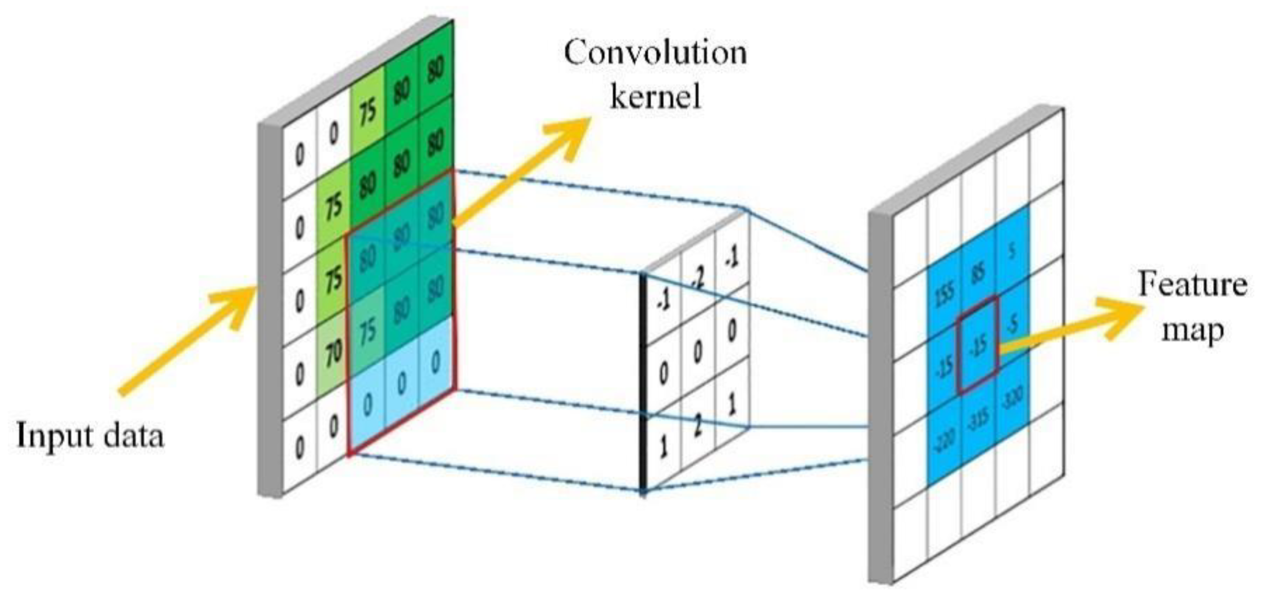
Figure 7 depicts the process to diagnose faults utilizing both optimized VMD and DTL, which consists of steps such as data preprocessing, the transformation of a two-dimensional time-frequency map, training network model, and fault classification. More detailed descriptions are given below.

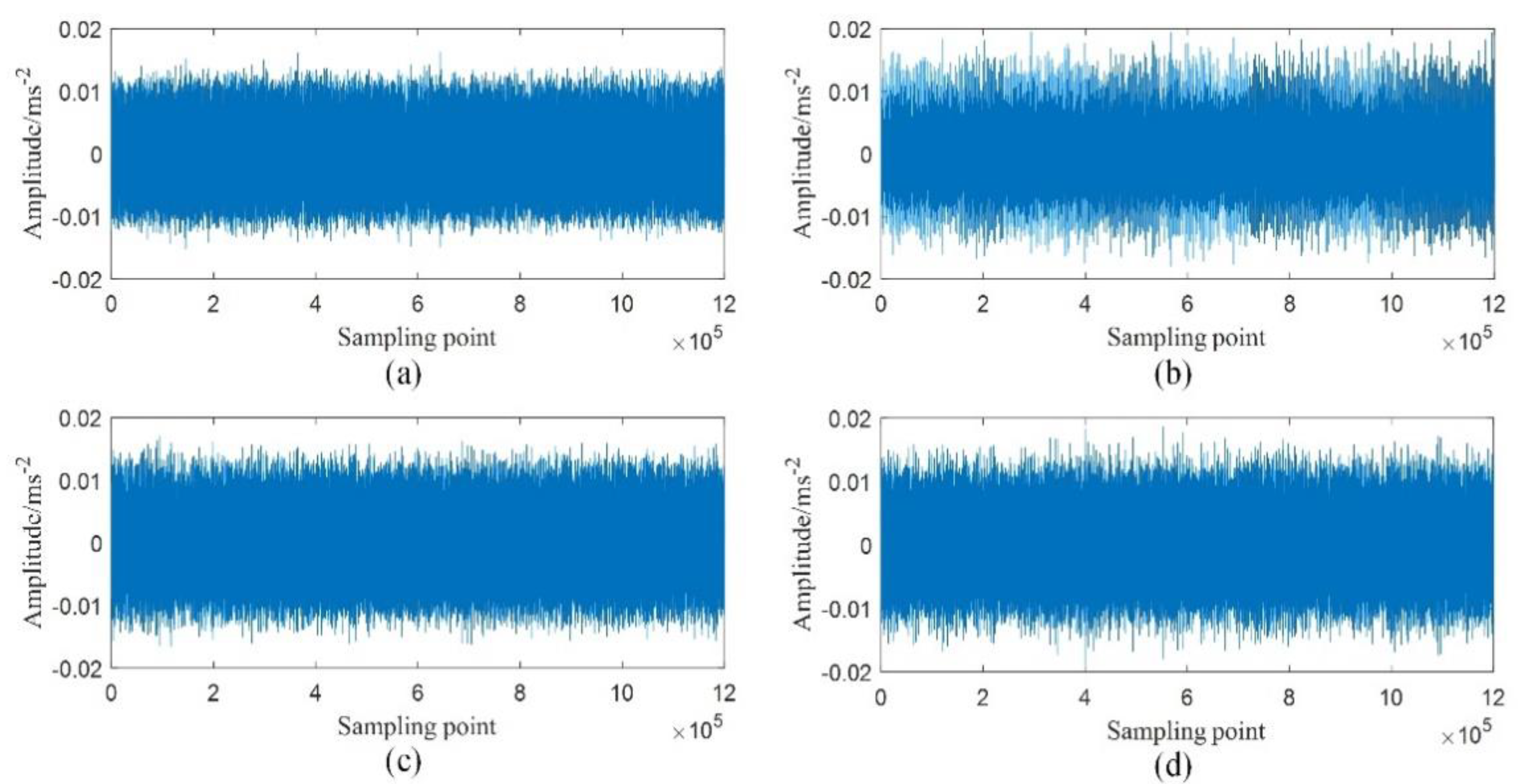
Step 1 Preprocess data. The VMD algorithm decomposes the original vibration signal, and the scatter entropy value of the IMF component is solved. When the change of dispersion entropy first appears as a turning point, the corresponding decomposition level is found to be the optimal decomposition level. The valuable information of the IMF component is screened out, according to the dispersive entropy value. Then, it is superimposed and reconstructed to obtain a noise reduction signal.

Step 2 Transform the two-dimensional time-frequency map. Taking the noise reduction signal as the input condition, the STFT algorithm is employed to produce the corresponding data set of the two-dimensional time-frequency graph. Then, training, testing, and validation sets are generated, respectively, when the data set is split.

Step 3 Train the network model. The parameters of the pre-trained ResNet18 network model are utilized as the transfer object. The parameters of the convolution 1 layer and the residual layer are frozen, and the fully connected layer is fine-tuned. Both training and test data sets are imported into the pre-trained model. The fine-tuned ResNet18 network model is retained to attain a novel DTL-ResNet18 network model.

Step 4 Classify Fault. The new test and validation data sets are imported into the trained ResNet18 network model. The Softmax activation function is utilized to obtain the final result of the fault diagnosis.

5. The Verification of the Experimental Data

5.1. Experiment Preparation

To verify the efficiency of the proposed method to diagnose faults of the diesel engine by employing both optimized VMD and DTL, an in-line 6-cylinder diesel engine test bench was established, which was composed of a panel monitoring condition, and data acquisition of the vibrational signal. A total of 6 vibration sensors were installed to collect data. Figure 8 depicts this.

During the actual operation of the diesel engine, the probability of failure of the fuel supply system is very high, which not only increases the maintenance cost but also brings great hidden dangers to production safety. Therefore, this paper mainly conducted detailed research on the system of the fuel supply, and preset four failure modes 1–4, as shown in

Table 1. The pre-set failure modes of the diesel engine.

Serial Numbers	Fault States	Failure Modes
1	L1	Normal
2	L2	Cylinder misfire
3	L3	Air filter clogged
4	L4	Broken oil supply pipe

. The specific three preset faults are shown in Figure 9.

5.2. Preprocessing and Analysis of the Experimental Data

The presented experiment was to collect effective vibration data. The rotational speed was uniformly set to 800 rpm. Then, 10 groups of data were collected for each failure mode. The frequency of the sampling was assigned to 20 kHz, and the collection time of each group was assigned to 12 s. The next set of data after a 30 s interval was collected.

Table 2. The datasets of the failures.

Fault State	Rotating Speed	Sampling Frequency	Sampling Time	Number of Sensors	Number of Samples
L1	800 rpm	20 kHz	12 s	6	10
L2	800 rpm	20 kHz	12 s	6	10
L3	800 rpm	20 kHz	12 s	6	10
L4	800 rpm	20 kHz	12 s	6	10

presents the detailed data collection parameters of the four preset failure modes. Figure 10 depicts the waveforms of the vibration data of the diesel engine in the four states.

When the characteristics of the diesel engine were taken into account, the data of sensor 4 was uniformly used as the verification of this experiment. Due to space issues, only the air filter clogging failure mode was employed as an illustrative example. The VMD decomposed the original vibration signal. Hence, the dispersion entropy of each IMF component was computed. Therefore, K, the end decomposition layer, was determined, and the parameter settings of the spreading entropy were determined. So, the number of categories were denoted by c = 8, the dimension by m = 2, and the time delay by d = 1, respectively. The larger the dispersion entropy of each IMF component, the higher the complexity would be. Besides, more complex interference signals and high-frequency noise signals would be obtained. The dispersion entropy of each component for the VMD decomposition layer was analyzed and the outcomes are presented in

Table 3. The analysis of the dispersion entropy for each component of the VMD decomposition.

IMF	The Dispersion Entropy of Each IMF Component When Various Ks Is Used
	3	4	5	6	7
IMF1	3.4637	3.5874	3.7228	3.5134	3.6991
IMF2	3.3146	3.4540	3.8595	3.6764	3.7245
IMF3	3.0940	3.2836	3.4521	3.6547	3.7565
IMF4		3.0683	3.2794	3.4482	3.4512
IMF5			3.0627	3.2768	3.2839
IMF6				3.0655	3.0765
IMF7					2.7068

when various K values were utilized. For example, K = 5 was the dispersive entropy of each component that had a turning point, indicating the utilization of components and noise components that appeared. Thus, the dispersive entropy of the IMF2 component was found to be the largest one indicating the complexity of the largest signal. Furthermore, the determination of the number of the VMD decomposition layers, which was K = 5, was found and the IMF components and spectrograms were eventually decomposed, as shown in Figure 11.

Figure 11b depicts that both IMF1 and IMF2 were high-frequency components with a complex spectrum and wide bandwidths. On the other hand, the IMF3, IMF4, and IMF5 components were selected as the basis for signal reconstruction when both inference signal and complex noise were taken into account. The STFT algorithm was employed to transform the denoised signal after reconstructing the two-dimensional time-frequency map data conducted by the VMD. The sampling length of each fault was uniformly set to 5000, and the size of the time-frequency map was uniformly assigned to 227 × 227 pixels. To meet the requirements of the DTL- ResNet18 network model for the input layer data, the specific two-dimensional time-frequency map data set is presented in

Table 4. The four preset fault time-frequency graph datasets of the VMD decompositions.

Signal States	Total Sample	Training Samples	Test Sample	Validation Sample
L1	240	180	20	40
L2	240	180	20	40
L3	240	180	20	40
L4	240	180	20	40
Total	960	720	80	160

.

5.3. The Comparative Analysis of the Noise Reduction Effect

To further verify the effectiveness of the noise reduction effect of the VMD method, the kurtosis value (K) and Peak Signal to Noise Ratio (PSNR) were selected to assess the effect of the noise reduction as indicators, which are defined by

$$K=\frac{\frac{1}{n}{\displaystyle {\sum }_{i=1}^n{(\left|x_i\right|-\mu )}^4}}{rm{s}^4}$$

(16)

The kurtosis could best represent the shock characteristics of the vibration signal, was more sensitive to the vibration shock, and was around 3 in the case of passing. If the deviation would be too large, it meant that the equipment was subjected to a certain vibration and shock, or there could a hidden danger of failure related to a key component.

$$PSNR=101g(z_{max}^2/(\frac{1}{N}{\displaystyle \sum _{j=1}^N{{\displaystyle (z_j-{z^{\prime }}_j)}}^2)})$$

(17)

where Z and Z’ denote the original and constructed vibration signals, respectively. PSNR is an important indicator directly reflecting the capacity of the noise reduction for the vibration signal. When PSNR became higher, a better noise reduction effect could be observed.

Table 2 presents the L4 fault data that was uniformly used to conduct validity. It can be seen from

Table 5. The contrastive analysis of the noise reduction with different modal decompositions.

Evaluation Indicators	Vibration Signal	CEEMD	EEMD	EMD	VMD
K-value	3.362	3.747	4.253	4.641	5.385
PSNR	4.253	15.652	18.368	24.527	32.983

that, after decomposing the vibration signal with strong noise by the VMD method, the kurtosis became the highest, indicating that the equipment deviated from the normal state, which was a more obvious characteristic of the fault. Thus, this suggested that the VMD method could eliminate strong noise signals and had a strong ability to retain fault features. When the PSNR index was compared with the CEEMD, EEMD, and EMD methods, the PSNR value of the VMD method reached up to 32.983. Hence, the higher the PSNR value, the better the noise reduction effect would be. Therefore, it was verified that the VMD method not only had a better noise reduction impact, but also reduced the difficulty of extracting fault features. Then, a basis to improve the accuracy of the fault diagnosis was provided in the next step.

5.4. The Setup and Training of the Network Model

The quality of the construction of the DTL-ResNet18 network model directly affected the final results of the fault classification. The detailed parameter settings for the training of the network model are shown in

Table 6. Setting the model parameters of the ResNet18 network.

Network Layer	Type	Size × Number of Output Channels	Output (Size × Number of Channels)
Input layer	RGB		227 × 227 × 3
Conv1	Convolutional Layer	7 × 7 × 54	114 × 114 × 64
Maxpool	Max Pooling Layer	3 × 3 × 64	57 × 57 × 64
Layer1	Residual Layer: IRB64 + IRB64	3 × 3 × 64	57 × 57 × 64
		3 × 3 × 64	57 × 57 × 64
		3 × 3 × 64	57 × 57 × 64
		3 × 3 × 64	57 × 57 × 64
Layer2	Residual Layer: SRB128 + SRB128	3 × 3 × 128	29 × 29 × 128
		3 × 3 × 128	29 × 29 × 128
		1 × 1 × 128	29 × 29 × 128
		3 × 3 × 128	29 × 29 × 128
		3 × 3 × 128	29 × 29 × 128
Layer3	Residual Layer: SRB256 + SRB256	3 × 3 × 256	15 × 15 × 256
		3 × 3 × 256	15 × 15 × 256
		1 × 1 × 256	15 × 15 × 256
		3 × 3 × 256	15 × 15 × 256
		3 × 3 × 256	15 × 15 × 256
Layer4	Residual Layer: SRB512 + SRB512	3 × 3 × 512	8 × 8 × 512
		3 × 3 × 512	8 × 8 × 512
		1 × 1 × 512	8 × 8 × 512
		3 × 3 × 512	8 × 8 × 512
		3 × 3 × 512	8 × 8 × 512
Avapool	Global average pooling layer	8 × 8 × 512	1 × 1 × 512
FC	Fully connected layer	1 × 1 × 4	4

. To verify the effectiveness of the training of the network model, the data set presented in Table 4 was utilized for verification. The t-distributed Stochastic Neighbor Embedding (t-SNE) method was employed to extract the image features of the pre-trained ResNet18 network model [36]. Then, the analysis of the data visualization was performed. Figure 12 depicts this.

Figure 12 depicts that extracting features related to faults in residual layer 1 could only distinguish the fault feature parameters of L2. On the other hand, the other three types of faults overlapped, thus, segregation became difficult. Then, the fault features extracted in the residual layer 2 could effectively distinguish the fault features of both L2 and L4. However, there still existed some fault features that had not been distinguished. When the fault features were extracted by residual layer 3, the fault features of both L1 and L3 also crossed each other. Eventually, the fault features extracted in the residual layer 4 could clearly distinguish four fault features, and the clustering effect was found to be good. Therefore, this could effectively suggest the effectiveness of the pre-trained ResNet18 network model to determine features for fault diagnosis with a strong ability to extract features.

Table 7. The pre-training diagnostic results of the VMD-ResNet18.

Network Model	Diagnostic Results				Training Time/S
	L1	L2	L3	L4
VMD-ResNet18	100.0%	100.0%	100.0%	100.0%	121.635 s

presents the better fault classification and processing capabilities of the pre-trained network model and its application status for the transfer of network models.

5.5. The Contrastive Analysis of the Decomposition Diagnosis Results with Various Modes

To further verify the pre-trained ResNet18 network model and the effectiveness of the optimized VMD method suggested in the manuscript, they were compared with the CEEMD, EEMD, and EMD algorithms, respectively. First, the original vibration signals were denoised by the VMD, CEEMD, EEMD, and EMD methods, respectively. Secondly, the reconstructed noise-reduced signal was transformed into a two-dimensional time-frequency graph by the STFT algorithm. The data set of each fault contained 180 training samples and 20 test samples, respectively. Finally, the pre-trained ResNet18 network model was uniformly employed to diagnose faults.

Table 8. The results of the contrastive analysis of the various mode decomposition diagnosis.

Fault State	Different Modal Decomposition Methods
	CEEMD	EEMD	EMD	VMD
L1	97.92%	100.0%	100.0%	100.0%
L2	100.0%	100.0%	100.0%	100.0%
L3	87.50%	95.83%	93.75%	100.0%
L4	93.75%	87.50%	95.83%	100.0%
Accuracy	94.79%	95.83%	97.40%	100.0%
Training time/s	166.744 s	137.427 s	153.226 s	121.635 s

presents the outcomes.

The diagnostic results suggested that the diagnostic accuracy of the VMD method reached 100%, and the lowest diagnostic result of the CEEMD was only 94.79% when compared to the three approaches. When the network training time was under consideration, the VMD algorithm had less training time than the others. Besides, the accuracy was higher, as shown in Figure 13. The verification results suggested that the proposed method could effectively remove both interference signals and complex noises. Hence, the extracted and reconstructed signal contained the required fault features, so that the pre-trained ResNet18 network model could obtain higher diagnostic accuracy.

5.6. Comparison and Analysis of Diagnosis Results of Different Network Models

To validate the effectiveness of the ResNet-18 network model, based on DTL proposed in this paper, AlexNet, SqueezeNet, and GoogLeNet network models were employed to make comparisons. The data set in Table 4 was used. The main network parameter settings of the four network models are shown in

Table 9. Comparing parameters of the four methods.

	ResNet18	AlexNet	SqueezeNet	GoogLeNet
Solver Name (Algorithm)	sgdm	sgdm	sgdm	sgdm
Initial Learn Rate	0.00005	0.00005	0.00005	0.00005
Max Epochs	10	10	10	10
Mini Batch Size	15	15	15	15
Validation Frequency	3	3	3	3
Shuffle	Every epoch	Every epoch	Every epoch	Every epoch
Execution Environment	GPU	GPU	GPU	GPU

.

From

Table 10. The comparison of the fault diagnosis of the different network models.

Network Model	Accuracy
	RAW DATA	CEEMD	EEMD	EMD	VMD
ResNet18	94.27%	94.79%	95.83%	97.39%	100.0%
AlexNet	88.02%	69.27%	79.16%	78.13%	95.31%
SqueezeNet	61.97%	65.10%	60.41%	71.35%	83.85%
GoogLeNet	62.50%	56.77%	41.14%	48.44%	76.56%

it can be seen that the accuracy rate of the ResNet18 network model reached 94.27% when the original data was directly used for 2D time-frequency map conversion. The accuracy ratio was higher when the comparison was made with the three approaches, which verified the effectiveness of the network model. After preprocessing of the IMF component of the original data by the VMD, the accuracy of the ResNet18 network model reached 100.0%, which was the highest when different modal decompositions were under consideration. The experimental results suggested that the VMD method had a better preprocessing ability when dealing with complex and strong noise signals. Besides, not only could the interference signal be effectively eliminated, but also higher diagnostic accuracy could be obtained. When both different network models and the unified network parameter settings were a concern, the ResNet18 network model had the best diagnostic results. However, the diagnostic results of the GoogLeNet network model did not achieve the same diagnosis effect. Therefore, both the effectiveness and feasibility of the ResNet18 network model once more were attained.

Both GoogLeNet and AlexNet network models showed stronger feature extraction and network learning capabilities when both classification and recognition were a concern. However, utilizing them for fault diagnosis cannot generate better outcomes when complex nonlinear vibration signals are under consideration, as, for example, with diesel engines. Figure 14 depicts that the method combining VMD and ResNet18 network model had better noise reduction performance and better diagnosis effect. The proposed method helped find a more efficient way of diagnosing faults of the diesel engine.

6. Conclusions

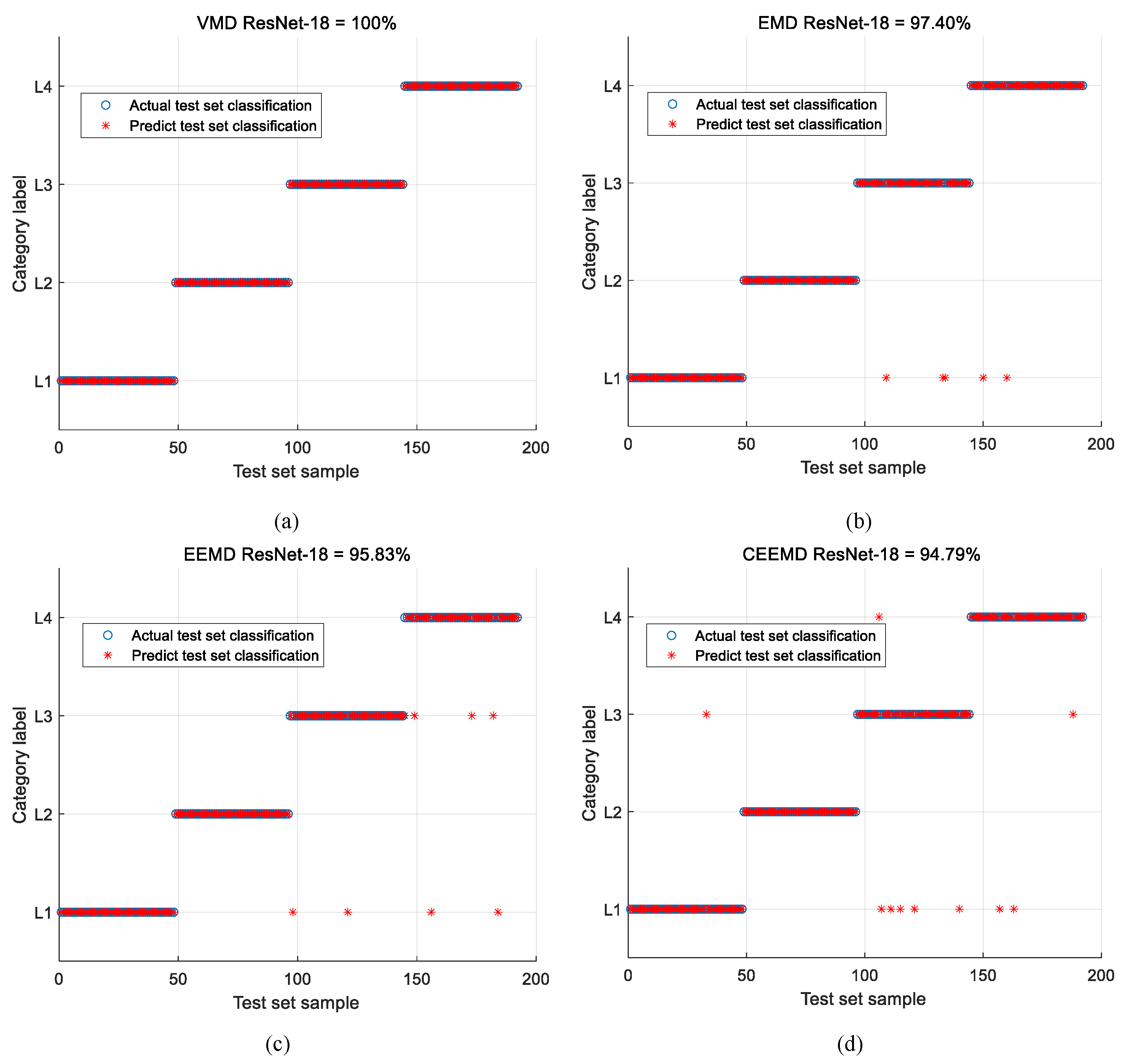
This research suggested an approach to diagnosing faults utilizing the combination of optimized VMD and DTL, concurrently. A successful transference of the pre-trained ResNet18 model on the ImageNet samples was conducted to diagnose faults of diesel engines in a more complex noise environment. The manuscript contributes the following:

(1) To decompose the level selection of the VMD, the level selection method of dispersive entropy was adopted and better noise reduction impact was attained.

(2) A two-dimensional time-frequency image processing problem with noise reduction was dealt with, after employing the STFT method to convert the one-dimensional vibration signal so as to extract features.

(3) An approach dependent upon the DTL was suggested. The ResNet-18 network was selected as the transfer object, and the network was fine-tuned. The proposed approach could directly derive key features of faults from two-dimensional time-frequency images and perform fault diagnosis. Thus, the difficulty of manually extracting features and the dependence on expert experience were reduced. Therefore, both diagnostic efficiency and accuracy were greatly improved.

The experiments showed that the implementation impact of the DTL concerning the diagnosis of faults for mechanical parts was better than other network models. As artificial intelligence technology advances rapidly, the DTL would play a key role in various engineering applications. Besides, the results of this research will help expand new knowledge in this field and have good reference value.

References

1. Wang, X.; Wang, T.; Ming, A.; Zhang, W.; Li, A.; Chu, F. Semi-supervised hierarchical attribute representation learning via multi-layer matrix factorization for machinery fault diagnosis. Mech. Mach. Theory 2022, 167, 104445. [Google Scholar] [CrossRef]
2. Ravikumar, K.N.; Yadav, A.; Kumar, H.; Gangadharan, K.V.; Narasimhadhan, A.V. Gearbox fault diagnosis based on Multi-Scale deep residual learning and stacked LSTM model. Measurement 2021, 186, 110099. [Google Scholar] [CrossRef]
3. Jung, D. Engine fault diagnosis combining model-based residuals and data-driven classifiers. IFAC-Pap. 2019, 52, 285–290. [Google Scholar] [CrossRef]
4. Luque, J.; Anguita, D.; Pérez, F.; Denda, R. Spectral analysis of electricity demand using Hilbert–Huang transform. Sensors 2020, 20, 2912. [Google Scholar] [CrossRef]
5. Gupta, N.; Seethalekshmi, K.; Datta, S.S. Wavelet-based real-time monitoring of electrical signals in Distributed Generation (DG) integrated system. Eng. Sci. Technol. Int. J. 2021, 24, 218–228. [Google Scholar] [CrossRef]
6. Xie, X.; Li, J.; Yin, F.; Xu, K.; Dai, Y. STFT based on bandwidth-scaled microwave photonics. J. Lightwave Technol. 2020, 39, 1680–1687. [Google Scholar] [CrossRef]
7. Samuel, P.D.; Pines, D.J. A review of vibration-based techniques for helicopter transmission diagnostics. J. Sound Vib. 2005, 282, 475–508. [Google Scholar] [CrossRef]
8. Liu, Z.; Qu, J.; Ming, J.Z. Fault level diagnosis for planetary gearboxes using hybrid kernel feature selection and kernel Fisher discriminant analysis. Int. J. Adv. Manuf. Technol. 2013, 67, 1217–1230. [Google Scholar] [CrossRef]
9. Anowar, F.; Sadaoui, S.; Selim, B. Conceptual and empirical comparison of dimensionality reduction algorithms (PCA, k-PCA, LDA, MDS, SVM, LLE, ISOMAP, LE, ICA, t-SNE). Comput. Sci. Rev. 2021, 40, 100378. [Google Scholar] [CrossRef]
10. Li, J.; Li, X.; He, D.; Qu, Y. A novel method for early gear pitting fault diagnosis using stacked SAE and GBRBM. Sensors 2019, 19, 758. [Google Scholar] [CrossRef] [Green Version]
11. Sun, H.; Guo, Y.; Zhao, W. Fault detection for aircraft turbofan engine using a modified moving window KPCA. IEEE Access 2020, 8, 166541–166552. [Google Scholar] [CrossRef]
12. Cheng, Y.; Yuan, H.; Liu, H.; Lu, C. Fault diagnosis for rolling bearing based on SIFT-KPCA and SVM. Eng. Comput. 2017, 34, 53–65. [Google Scholar] [CrossRef]
13. Wang, Z.; Zhang, Q.; Xiong, J.; Xiao, M.; Sun, G.; He, J. Fault diagnosis of a rolling bearing using wavelet packet denoising and random forests. IEEE Sens. J. 2017, 17, 5581–5588. [Google Scholar] [CrossRef]
14. Baraldi, P.; Cannarile, F.; Di Maio, F.; Zio, E. Hierarchical k-nearest neighbors classification and binary differential evolution for fault diagnostics of automotive bearings operating under variable conditions. Eng. Appl. Artif. Intell. 2016, 56, 1–13. [Google Scholar] [CrossRef] [Green Version]
15. Bi, X.; Lin, J.; Tang, D.; Bi, F.; Li, X.; Yang, X.; Ma, T.; Shen, P. VMD-KFCM algorithm for the fault diagnosis of diesel engine vibration signals. Energies 2020, 13, 228. [Google Scholar] [CrossRef] [Green Version]
16. Chen, K.; Mao, Z.; Zhao, H.; Jiang, Z.; Zhang, J. A variational stacked autoencoder with harmony search optimizer for valve train fault diagnosis of diesel engine. Sensors 2019, 20, 223. [Google Scholar] [CrossRef] [Green Version]
17. Gu, C.; Qiao, X.Y.; Li, H.; Jin, Y. Misfire fault diagnosis method for diesel engine based on MEMD and dispersion entropy. Shock. Vib. 2021, 2021, 9213697. [Google Scholar] [CrossRef]
18. Jia, F.; Lei, Y.; Lin, J.; Zhou, X.; Lu, N. Deep neural networks: A promising tool for fault characteristic mining and intelligent diagnosis of rotating machinery with massive data. Mech. Syst. Signal Processing 2016, 72, 303–315. [Google Scholar] [CrossRef]
19. Shang, C.; Yang, F.; Huang, D.; Lyu, W. Data-driven soft sensor development based on deep learning technique. J. Process Control. 2014, 24, 223–233. [Google Scholar] [CrossRef]
20. Lei, Y.; Jia, F.; Lin, J.; Zhou, X.; Lu, N. An intelligent fault diagnosis method using unsupervised feature learning towards mechanical big data. IEEE Trans. Ind. Electron. 2016, 63, 3137–3147. [Google Scholar] [CrossRef]
21. Zhang, J.; Tian, Y.; Ren, Z.; Chang, Q.; Jia, Z. The calibration of force offset for rocket engine based on deep belief network. Meas. Control. 2018, 51, 172–181. [Google Scholar] [CrossRef]
22. Wang, Y.S.; Liu, N.N.; Guo, H.; Wang, X.L. An engine-fault-diagnosis system based on sound intensity analysis and wavelet packet pre-processing neural network. Eng. Appl. Artif. Intell. 2020, 94, 103765. [Google Scholar] [CrossRef]
23. Xu, J.; Liu, X.; Wang, B.; Lin, J. Deep Belief Network-Based Gas Path Fault Diagnosis for Turbofan Engines. IEEE Access 2019, 7, 170333–170342. [Google Scholar] [CrossRef]
24. Zhou, D.; Yao, Q.; Wu, H.; Ma, S.; Zhang, H. Fault diagnosis of gas turbine based on partly interpretable convolutional neural networks. Energy 2020, 200, 117467. [Google Scholar] [CrossRef]
25. Han, P.; Ellefsen, A.L.; Li, G.; Æsøy, V.; Zhang, H. Fault Prognostics Using LSTM Networks: Application to Marine Diesel Engine. IEEE Sens. J. 2021, 21, 25986–25994. [Google Scholar] [CrossRef]
26. Xu, W.; Wan, Y.; Zuo, T.Y.; Sha, X.M. Transfer learning-based data feature transfer for fault diagnosis. IEEE Access 2020, 8, 76120–76129. [Google Scholar] [CrossRef]
27. Zhao, Y.P.; Chen, Y.B. Extreme learning machine-based transfer learning for aero-engine fault diagnosis. Aerosp. Sci. Technol. 2022, 121, 107311. [Google Scholar] [CrossRef]
28. Xiong, G.; Ma, W.; Zhao, N.; Zhang, J.; Jiang, Z.; Mao, Z. Multi-type diesel engines operating condition recognition method based on stacked auto-encoder and feature transfer learning. IEEE Access 2021, 9, 31043–31052. [Google Scholar] [CrossRef]
29. Zhou, M.; Hu, T.; Bian, K.; Lai, W.; Hu, F.; Hamrani, O.; Zhu, Z. Short-Term Electric Load Forecasting Based on Variational Mode Decomposition and Grey Wolf Optimization. Energies 2021, 14, 4890. [Google Scholar] [CrossRef]
30. Cai, W.; Yang, Z.; Wang, Z.; Wang, Y. A new compound fault feature extraction method based on multipoint kurtosis and variational mode decomposition. Entropy 2018, 20, 521. [Google Scholar] [CrossRef] [Green Version]
31. Azami, H.; Escudero, J. Amplitude-and fluctuation-based dispersion entropy. Entropy 2018, 20, 210. [Google Scholar] [CrossRef] [PubMed] [Green Version]
32. Khetarpal, P.; Tripathi, M.M. A critical and comprehensive review on power quality disturbance detection and classification. Sustain. Comput. Inform. Syst. 2020, 28, 100417. [Google Scholar] [CrossRef]
33. He, K.; Zhang, X.; Ren, S.; Sun, J. Deep residual learning for image recognition. In Proceedings of the IEEE Conference on Computer Vision and Pattern Recognition, Las Vegas, NV, USA, 12 December 2016; pp. 770–778. [Google Scholar]
34. Hao, X.; Zheng, Y.; Lu, L.; Pan, H. Research on Intelligent Fault Diagnosis of Rolling Bearing Based on Improved Deep Residual Network. Appl. Sci. 2021, 11, 10889. [Google Scholar] [CrossRef]
35. Ma, P.; Zhang, H.; Fan, W.; Wang, C.; Wen, G.; Zhang, X. A novel bearing fault diagnosis method based on 2D image representation and transfer learning-convolutional neural network. Meas. Sci. Technol. 2019, 30, 055402. [Google Scholar] [CrossRef]
36. Agis, D.; Pozo, F. Vibration-Based Structural Health Monitoring Using Piezoelectric Transducers and Parametric t-SNE. Sensors 2020, 20, 1716. [Google Scholar] [CrossRef] [PubMed] [Green Version]
Figure 1. The schematic diagram of the basic principle of the STFT.
Electronics 11 01969 g001
Figure 2. The schematic diagram of the convolution process.
Electronics 11 01969 g002
Figure 3. Schematic diagram of max pooling operation.
Electronics 11 01969 g003
Figure 4. The residual structure of the block diagram: (a) Indentity residual block; (b) Sampling residual block.
Electronics 11 01969 g004
Figure 5. The schematic diagram of the global average pooling.
Electronics 11 01969 g005
Figure 6. The schematic diagram of the model migration process.
Electronics 11 01969 g006
Figure 7. The process to diagnose faults of the diesel engine employing optimized VMD and DTL.
Electronics 11 01969 g007
Figure 8. The test rig of the planetary gearbox.
Electronics 11 01969 g008
Figure 9. The preset failure modes: (a) Ring gear, (b) Planet gear, (c) Sun gear.
Electronics 11 01969 g009
Figure 10. The vibration waveforms of the diesel engine for 4 different states: (a) L1 state; (b) L2 state; (c) L3 state; (d) L4 state.
Electronics 11 01969 g010
Figure 11. The VMD decompositions: (a) each IMF component; (b) each IMF component spectrogram.
Electronics 11 01969 g011
Figure 12. The t−SNE visualization analysis of the VMD−ResNet18 network for feature extraction.
Electronics 11 01969 g012
Figure 13. The results of the contrastive analysis of the different mode decomposition diagnoses: (a) VMD = 100%; (b) EMD = 97.4%; (c) EEMD = 95.83%; (d) CEEMD = 94.79%.
Electronics 11 01969 g013
Figure 14. The fault diagnosis results of the different network models: (a) Raw data = 94.27%; (b) VMD-ResNet18 = 100%; (c) EMD-ResNet18 = 97.39%; (d) EED-ResNet18 = 95.83%; (e) CEED-ResNet18 = 94.79%.
Electronics 11 01969 g014