MEAN: Multi-Edge Adaptation Network for Salient Object Detection Refinement

Abstract

Recent advances in salient object detection adopting deep convolutional neural networks have achieved state-of-the-art performance. Salient object detection is task in computer vision to detect interesting objects. Most of the Convolutional Neural Network (CNN)-based methods produce plausible saliency outputs, yet with extra computational time. However in practical, the low computation algorithm is demanded. One approach to overcome this limitation is to resize the input into a smaller size to reduce the heavy computation in the backbone network. However, this process degrades the performance, and fails to capture the exact details of the saliency boundaries due to the downsampling process. A robust refinement strategy is needed to improve the final result where the refinement computation should be lower than that of the original prediction network. Consequently, a novel approach is proposed in this study using the original image gradient as a guide to detect and refine the saliency result. This approach lowers the computational cost by eliminating the huge computation in the backbone network, enabling flexibility for users in choosing a desired size with a more accurate boundary. The proposed method bridges the benefits of smaller computation and a clear result on the boundary. Extensive experiments have demonstrated that the proposed method is able to maintain the stability of the salient detection performance given a smaller input size with a desired output size and improvise the overall salient object detection result.

1. Introduction

Salient object detection is a prominent first step for various computer vision applications to produce a coarse detection. Given an image, the salient detection provides the guidance on the image region that requires attention. This technique can be immediately applied in many applications such as visual tracking, image captioning [1,2,3], image segmentation [4,5,6,7,8,9,10,11], and visual question answering [12,13].

The advances in deep learning architectures [14,15,16,17] have made them widely used feature extractors in many computer vision applications. In addition, the deep learning has been gaining a lot of attention for the improvement of saliency prediction in recent years. The utilization of deep learning in saliency models can effectively imitate the attention mechanism of human vision compared with handcrafted features, as proposed in [18]. Several approaches that utilize the edge prediction as the additional feature have been proposed. A mutual learning module is proposed in [19] to incorporate edge prediction with saliency detection. The multitask intertwined supervision is used to train this module. This work shows the mutual benefit between nested edge prediction and salient object prediction. The predicted edge gradually enhances the accuracy by integrating the additional boundary prediction to precisely locate the boundary of the salient object. A cascaded partial decoder is proposed in [20], in which only features of the deeper layers are integrated in the decoder. A holistic attention module is utilized to combine the features from the initial prediction to the final prediction of the partial decoder. Another approach utilized refinement and improved it with the top-down and bottom-up approach [21]. The result from the saliency is refined using a Recurrent Neural Network (RNN) in top-down order using the convolutional feature from coarse prediction. Subsequently, these features are refined again in a bottom-up order using both convolution and refined saliency from the previous top-down approach. Some other works also utilize side-outputs during training as [22] and have shown the effectiveness of the single refinement process, which is able to refine the coarse saliency maps into a more precise boundary such as BASNet [23] that used Fully Convolutional Network (FCN)-based architecture as the refined network. In BASNet, the refinement network predicted the residual image that refined the coarse map through element-wise summation. In addition, the Conditional Random Field (CRF) [24] and Recurrent network [25] also can provide good results with additional computation.

As the first step in vision tasks, fast saliency detection is highly demanded. Conversely, the CNN involves a lot of computation which slows down the process. Specifically, most of the CNN-based salient detectors adopt a backbone network which contains many layers of convolution. This arrangement becomes non-trivial when receiving a large image. This obstacle has been addressed by utilizing the downsampling trick, in which the input was resized into a smaller size, and the result was upsampled back to its original size. This arrangement is referred to as “bottleneck prediction” in this study. The bottleneck prediction approach reduces the computation significantly, yet the results are less accurate when the bilinear interpolation is adopted as the post processing. For instance, when an image of size 512 $\times$ 512 is resized into a smaller image of size 256 $\times$ 256, it is termed as the temporal size. Subsequently, it is fed to the CNN with symmetrical encoder-decoder architecture to obtain a result of size 256 $\times$ 256. To obtain a similar size as the input, this saliency result is upsampled into 512 $\times$ 512. Normally, this approach achieves a good result when the original image size is close to 256 $\times$ 256. However, when the image size is much larger than this size, such as 1028 $\times$ 1028, the salient detector degrades its performance.

The edge detection-based approach enhances the accuracy by adding additional boundary prediction to precisely locate the boundary of the salient object. Edge prediction is deployed in each stage of the encoder. This forms the nested edge detection, which is beneficial for the prediction. However, the original input size is needed for this approach to predict a more accurate edge in every encoder stage. Unfortunately, the encoder is mostly composed of the backbone network which requires a lot of computation. The bottleneck prediction approach does not work well with this structure, in which the edge prediction, which is produced as a side output, is not accurate enough to represent the real gradient of the original image. Due to the inaccurate boundaries, the predicted edge in the aforementioned case is less beneficial for refinement purposes. In addition, the predicted edges are only available with limited sizes up to the defined temporary size which is still smaller than the original image size. This means that the predicted edges are only available with limited sizes up to the defined temporary size. To overcome this limitation, the predicted edge needs to be upsampled to the same size as that of the saliency result, leading to thicker and inaccurate boundaries in the result.

To overcome this issue, the refinement-based approach is a good option that works well with the bottleneck prediction scheme. The two modules must collaborate, with one of the modules acting as the predictor and the other as the refinement. This mechanism can effectively reduce the computation, and still provide better results. In this process, a robust refinement module is highly demanded. Since the prediction size is smaller than that of the original image size, the refinement module must be able to adapt with the change of object size inside the image. Thus, to enhance the refinement, the original image gradient is utilized as guidance for the refinement. The gradient image is obtained is of the original image size to provide more precise boundary information for the refinement process.

In this study, a novel salient object detection is proposed, in which the coarse salient object is predicted by the prediction module, and subsequently refined by a light CNN with the image gradient of the original size. The contributions of this work are summarized as follows.

• A transition module is proposed to use the original image gradient as the additional input for refinement purposes.
• A 3D convolution, termed the ‘channel domain analyzer’, is adopted to handle the feature map relationships in different channels.
• Applying the training mechanism to improve the performance of the existing salient detection network by using the original image gradient.
• Introducing various refinement strategies for better saliency results.

The remainder of this paper is organized as follows. Some related works are reviewed in Section II. Section III elaborates the components and the process of the proposed MEAN in detail. Extensive experimental results and discussions are reported in Section IV. Section V draws the conclusion.

2. Related Works

Many approaches have been proposed prior to deep learning using classical block-based and region-based analysis. However, recently deep learning has been adopted for its ability to solve the salient problem through learning. Specifically, the FCN-based method is the most popular with many variations and improvements. One popular improvement is the encoder–decoder architecture. The design of an encoder can be VGGNet [14] or ResNet [17]. The fully convolutional network can also be extended into a recurrent-type approach [25].

Attention mechanisms are widely used in natural language processing and caption generation. The Squeeze and Excitation Network [26] shows a basic idea utilizing the attention mechanism both in channel and spatial domains with global average pooling which improves the accuracy in recognition. The Convolutional Block Attention Module (CBAM) deploys the fully convolutional networks to deal with the channel attention, in which it handles both spatial and channel domains separately and combines the features for robust recognition. Both methods have shown that deploying an attention model in the network is able to improve the performance of the CNN by paying more attention or weighting the most important feature maps for a specific task. In [18], a multilevel deep neural network (DNN) with an identity block is proposed. This design is also strengthened by a semantic perception subnetwork, in which it can capture potential saliency regions and possible high-level semantic information in an image. Both of these modules allow the network to obtain the robust and accurate feature for saliency map generation.

Improving the saliency accuracy from the coarse map has been widely adopted. Most of the saliency algorithms employ three types of refinements, i.e., Conditional Random Field (CRF) [24], Convolutional Neural Network, and Recurrent Neural Network. The CNN type layer can be a single convolutional layer or adopting FCN again with the encoder-decoder as in BASNet [23], which is able to generate promising salience boundary. However, this approach is not trained to perform in various sizes for refinement. This condition refers to BASNet feeding the same image input size for both its prediction module and residual refinement module. In MLMSNet [19], it has been proven that supervision plays an important role for the model, in particular for edge supervision. However, this approach does not address the refinement across various scales. Thus, in this work, the edge feature is utilized to guide the refinement of the saliency result for better saliency contours.

3. Proposed Method

The proposed method consists of three components, i.e., prediction, transition, and refinement modules. The prediction module acts as the base predictor that captures the important object shape, structure, and determines the salient object area in the downsampled size. The refinement module transforms the coarse saliency map to a better result. The transition module serves as the bridge for the additional edge feature with the coarse map before refinement. Figure 1a illustrates the overall flow of the proposed Multi-Edge Adaptation Network (MEAN).

3.1. Salient Object Detection Mechanism

With the intensive development of deep learning for salient object detection, a lot of techniques were introduced. Yet, they share one common mechanism, in which the input image is directly fed to the CNN to predict the salient object and background classes. Let us assume that I is the input image and S is the salient detection result. Meanwhile, the bottleneck prediction approach utilizes a different method, in which I is first resized to a predefined temporary size I_R. Subsequently, I_R is fed to the CNN network to produce the prediction S_R. At the last stage, S_R is resized to the original image size to form the final prediction S. The framework introduces several issues: (1) It is infeasible for a network to capture the details because the prediction result, S_R, lacks many details when it is upsampled into S, in particular when a large size difference exists between S and S_R. (2) It is necessary to have a module that is sufficiently robust to refine the result from S_R to S. Since the image may contain complex boundaries, the refinement needs to adapt this type of boundary into a coarse map, S_R, that is usually inaccurate due to the downsampling process. (3) A huge computation can be introduced when a large I is fed to the network, slowing down the training and increasing memory consumptions.

Another reason for applying the bottleneck prediction is that the salient object tends to be located in the center and is normally the biggest object in the image. By downsampling the image, it can increase the receptive field of the kernel in the convolution operation by widening the field of view to capture a bigger object inside the image. With a smaller spatial dimension, the computational complexity is reduced, yet it may introduce inaccuracy to boundary of the S_R.

As shown in Figure 1a, the MEAN consists of the predictor module (${\phi }_P$) which is composed of the encoder (E(i)) and decoder (D(i)) with side output (O(i)), transition module (${\phi }_T$) and the refinement module (${\phi }_R)$. The MEAN adopts the original image gradient to serve as the guidance of the refinement. The training scenario of the MEAN is designed to produce a robust refinement network, in which the transition and refinement modules are purposely incorporated at each side output.

Consequently, as opposed to the general encode–decode salient detector, the bottleneck prediction can be handled with the MEAN in several ways: (1) refining the S_R to S with the refinement network, (2) designing the decoder with progressive (sequential refinement) feature, and (3) using refinement network to refine S_R after a huge upsampling operation (skip refinement), as shown in Figure 2.

In the first approach, the refinement network which is used to refine the coarse map is introduced in BASNet [23]. A similar approach is also employed in this study. Yet, in this study the edge is extracted from the original image as guidance for the training of the refinement network. There are three different refinement mechanisms as follows and as described in Figure 2.

3.1.1. Basic Refinement (BR)

The first is the Basic Refinement (BR) stage, in which all of the modules, i.e., prediction, transition, and refinement are with the same input size. This refinement mechanism is widely adopted in former schemes such as BARNet [23]. In the BR case, the refinement is only equipped in the O₇ with no upsampling operation involved. This condition indicates that the model only works at a single scale. Thus, the processing time increases a lot because the input of the prediction module is not downsampled.

3.1.2. Sequential Refinement (SQR)

The second approach is the sequential refinement (SQR), in which the coarse map that has been refined at certain scales is upsampled and refined again to produce a better result at higher scales. Let R be the set of scales which contains r number of scales, the proposed framework produces r results as prediction S = {S₁, S₂, S₃, …, S_r}, termed as Sequential Refinement (SQR). For instance, the image I has a certain scale R_(i), and R_(i−1) and S_(i−1) are downsampled result and saliency result of I, respectively. The edge, E, is generated from I at scale R_(i). The S_(i−1) is upsampled from R_(i−1) to R_(i) and incorporated with E to obtain S_(i) in scale R_(i). Thus, the upsampled S_(i−1) defines the salient area, and subsequently the refinement network ${\phi }_{REF}$ adjusts it using E for a better contour. Since the Sobel operator can produce the image gradient E in any size, this approach can be conducted multiple times. The progressive approach can also be utilized to refine the coarse map from any side output in the decoder stages. The computational complexity depends on how many times the refinement is applied. It will consume more time when the refinement is frequently conducted.

3.1.3. Skip Refinement (SKR)

The last refinement type is skip refinement (SKR). The SKR skips some refinement processes in SQR. The refinement process is only placed in the final scale instead of applying progressively, as in SQR. In addition, instead of producing r results, the method skips some scales. For instance, refining S₁ in scale R₍₁₎ into S₄ in scale R₍₄₎ involves a three-times upsampling process. Compared to the SQR, SKR is with a lower computational complexity, because the refinement process is only performed once instead of multiple times. The final scale in this scenario refers to the original image size. The SKR incorporates the edge at the final size r, denoted as $E_{\left(r\right)}$, and the coarse map upsamples n times for the refinement process, as in Equation (7). The performance of SKR gets worse when the final size and temporary size have a large difference.

3.2. Edge Detector

The directional change of the intensity in an image is widely utilized to detect the image gradient. Many algorithms have been proposed for edge detection using deep learning such as HED [22]. This method has also been applied in salient object detection as additional information for the decoder, as in [19,21]. This approach has drawbacks in bottleneck prediction. Specifically, the predicted edge in a smaller size of feature map cannot be a good feature to guide the refinement at higher scales due to its inaccurate boundaries.

For instance, the encoder ${\phi }_{ENC}$ with n stages is only capable of giving n edges information for refining. Due to the downsampling process utilized in the bottleneck prediction approach, this predicted edge is resized back to its original size. Yet, when the scale difference between the input image and predicted edge is too large, many contour details are missing. Another issue that may arise is that the training relies on the availability of a dataset containing a huge amount of both edge information and salient detection with accurate labeling.

Consequently, in this study, the conventional Sobel edge detection is utilized. The Sobel was chosen due to its simplicity with low computational complexity. In general, the bottleneck prediction needs refinement in the bigger scale. Using Sobel, the computation can be reserved because it only contains two convolution operations along x and y directions with 1 $\times$ 3 and 3 $\times$ 1 kernels, respectively. However, it has a drawback in that it returns very noisy edges, some of which can be related to the salient mask, but most of which are unwanted edge results. Consequently, the detected edge result is fed to the transition module which will be discussed in the next section.

3.3. Prediction Module

Let ꭓ be the feature maps produced by a composite function $\phi$. The MEAN predictor module (${\phi }_P$) adopts the encoder–decoder architecture. The encoder ${\phi }_{ENC}$ contains several convolutional layers, followed by the batch normalization and ReLU activation function, which are grouped into n stages, ${\phi }_{ENC}=\left\{{\phi }_{E1}, {\phi }_{E2},{\phi }_{E3},\dots ,{\phi }_{En}\right\}$, and it produces n feature maps, denoted as ${ꭓ}_{ENC}=\left\{{ꭓ}_{E1}, {ꭓ}_{E2},{ꭓ}_{E3},\dots ,{ꭓ}_{En}\right\}$. The term ‘stage’ refers to the set of operations, including convolution, batch normalization and activation function, before the pooling operation. In this study, ResNet 34 [17] is employed as the encoder. Inspired by BASNet [23], the first input layer of the encoder is modified to a 3 × 3 filter with no pooling. In addition, there are two additional stages after the fourth stage, which contains three residual blocks (512 filters) after the max pooling operation. The variable n is the number of ${\phi }_{ENC}$ stages, and the decoder ${\phi }_{DEC}$ normally has identical stages to those of the encoder. Inspired by UNet [4], the skip connection is utilized to refine the decoder-reconstructed result and the design of the decoder is expected to be symmetrical. The ${\phi }_P$ also adopts the deep supervision training style which generates a prediction $\left\{O_1, O_2,O_3,\dots ,O_7\right\}$ for each decoder stage as the side output as shown in Figure 1a.

3.4. Transition Module

During the refinement step, the original image edge is utilized as an additional input to the refinement network. However, the edges detected by Sobel not only contain the salient contour, but also contain other objects which are not related to the salient object. Consequently, an additional screening process is needed before feeding the detected edge as an additional feature. Inspired by the SE Networks [26] and CBAM [27], the transition module is designed in this study to handle the feature in the spatial and channel domains. In the spatial domain, the method pays attention to the objects inside the image. In addition, in the channel domain, the method emphasizes the relation between the generated feature maps in a depth-wise manner.

3.4.1. Spatial Domain Analyzer

In analyzing the spatial domain, 2D convolution is adopted. The most challenging task in this domain is the ability of the convolution to capture most of the object features, meaning suitable receptive fields of the convolution should be adopted in various scales. For instance, in a small image, e.g., 64 × 64, a 3 $\times$ 3 convolution is able to capture the object inside the image. Yet, when the size of the image increases to 512 $\times$ 512, a convolution receptive field of size 3 $\times$ 3 is unable to capture the shape of the object as it can only see a small portion of the object.

$${ꭓ}_{pool2}={\phi }_{pool2}\left(Av{g}_{pool2}\left({ꭓ}_{inp}\right)\right)$$

(1)

$${ꭓ}_{pool4}={\phi }_{pool4}\left(Av{g}_{pool4}\left({ꭓ}_{inp}\right)\right)$$

(2)

To overcome this problem and generate a more robust feature that is invariant to the various object sizes inside the image, multiple pooling operations are incorporated with 2 $\times$ 2 of stride 2, as in Equation (1), and 4 $\times$ 4 stride 4 pooling in Equation (2). The average pooling is used to downsize the feature map input ${ꭓ}_{in}$. Both of the features are later processed by ${\phi }_{pool2}$ and ${\phi }_{pool4}$ layers that consist of a single 3 $\times$ 3 convolution followed by the batch normalization and ReLU activation function. Thus, the network is able to handle various scales, and make decisions based on the combinations of them. The operations, ${\phi }_{pool2}$ and ${\phi }_{pool4}$, are applied after the pooling operation, as shown in Figure 3.

In addition, the original ${ꭓ}_{in}$ is also analyzed using ${\phi }_{in}$, and the generated feature map is combined using the element-wise summation, as in Equation (3). Subsequently, it is fed to the 3 × 3 convolution for generating ${ꭓ}_{final}$, as in Equation (4). As a result, it widens the field of view (FOV) and increases the chance of the convolution kernel capturing a bigger object in the image. This operation is termed ‘pooling convolution’ in the rest of the section.

$${ꭓ}_{sum}={\phi }_{in}\left({ꭓ}_{in}\right) +{ꭓ}_{pool2}+{ꭓ}_{pool4}$$

(3)

$${ꭓ}_{final}={\phi }_{fin}\left({ꭓ}_{sum}\right)$$

(4)

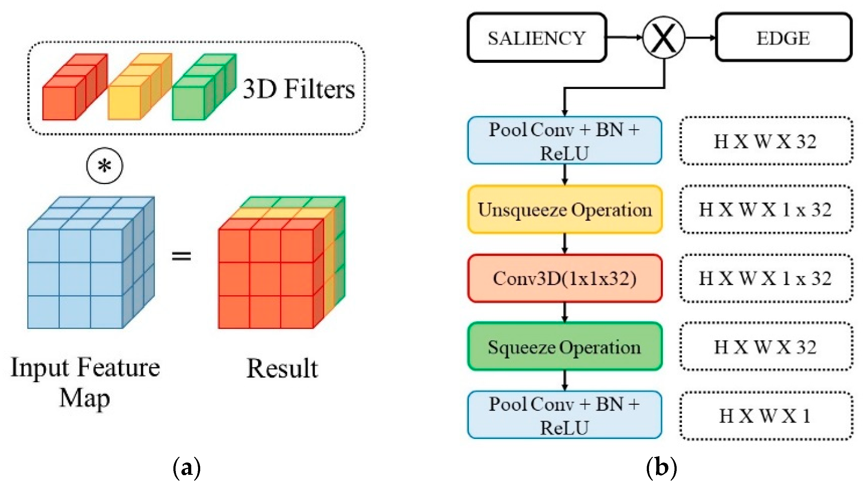
3.4.2. Channel Domain Analyzer

In the channel domain, the main focus is to capture the relation channel-wise. The transition layer maps the relationship between the upsampled coarse map and the edge, E, in the higher scale size. This relation can only be captured in the channel relation. In SE networks, the global average pooling operation is applied in each channel to produce a single number in each channel instance. To capture a more detailed channel relation, the fully connected layer is applied to the pooled feature maps. The output of the FC layer indicates the attenuator value for different channels, which is termed the ‘feature descriptor’. In addition, in the CBAM channel attention module, the max pooling and average pooling operations are performed to produce two feature maps. The two feature maps have a different FC layer for capturing the channel relation in max and average operations. Thus, for the SE network, it only provides one channel relation, while there are two channel relations in CBAM.

These mechanisms have drawbacks that the global pooling operation losses a lot of spatial information. Instead of using the global pooling operation to produce a single number as a feature representation, the 3D convolution is applied. Yet, the difference is that the size of the 3D convolution is (1 $\times$ 1 $\times$ D) where D is equivalent to the channel of the feature maps. The number of the filters in the 3D convolution also represents a different relation that may occur in the feature maps, and it is set at 16 in this study. The 16 kernels represent 16 various relations of the channels, as described in Figure 4a.

Given an intermediate feature map ${ꭓ}_{in}$∈ R^CXHXW as the input, the channel domain analyzer ${\phi }_{CDA}$ transforms ${ꭓ}_{in}$ to ${ꭓ}_{CDA}$∈ R^CXHXW with the 3D convolution kernel K ∈ R^CX1X1. Let H and W be the height and width, respectively; C is the channel and N is the batch number of the feature maps. The single 3D convolution is with depth D. In practice, the feature map with size {N, C, H, W} is transformed to a five-dimensional tensor with a depth as the additional information with format {N, C, D, H, W} where C is equal to 1. This operation is termed the ‘unsqueeze’ operation. The five-dimensional tensor is fed to the 3D CNN with kernel size (1 $\times$ 1 $\times$ D), producing the feature map {N, 1, D, H, W}. Subsequently, this five-dimensional tensor is reshaped into {N, C, H, W}, where C = D is termed the ‘squeeze’ operation.

3.4.3. Transition Module

The proposed transition module is the combination of channel and spatial domain analyzer. However, prior to channel attention, another convolution is applied to expand the channel size, producing more comprehensive information to be processed in both the channel and spatial domains. In this study, a similar pooling convolution for spatial domain process is utilized to produce an intermediate channel with size 32. Figure 4b illustrates the detailed architecture. The topmost layer is the spatial analyzer which is another pooling convolution with output size 1 for generating the filtered edge map. During the training, the transition module is placed after the side output O₄, 0₅, and O₆ to capture various upsampling ratios. All of the transition modules share the same weighting. To produce the filtered edge map, ${ꭓ}_{T\left(i\right)}$, the upsampled coarse map, ${ꭓ}_{S\left(i-1\right)}$, and edge, E_(i), are needed, in which i is the step, indicating the current size and U is the upsampled operation, as in Equation (5).

$${ꭓ}_{T\left(i\right)}={\phi }_T\left(E_{\left(i\right)}\otimes U\left({ꭓ}_{S\left(i-1\right)}\right)\right)$$

(5)

3.5. Refinement Module

Similar to the transition module, the refinement module works on the original image size. The main differences with BASNet [23] are in the input and output. The MEAN refinement module receives both adapted image gradient from transition module and the saliency coarse map. In addition, for the output, as opposed to predicting the residual image, the refinement module in this study predicts the salient map directly without the element-wise summation at the end as shown in Figure 1b.

During the training, the refinement module is placed after the transition module. Herein, a huge advantage can be obtained during the training because the upsampling factor in T₅ is 4, and it is 2 in T₆. No upsampling is arranged in T₇. This variety serves as the data augmentation, in which the refinement module is able to detect a different input at a different scale factor. The refinement networks in R₅, R₆, and R₇ share the same weighting. The refinement process always needs the result of the transition module as in Equation (6), in which ⊗ is a concatenation operation.

$${ꭓ}_{R\left(i\right)}={\phi }_R\left({ꭓ}_{T\left(i\right)}\otimes U\left({ꭓ}_{S\left(i-1\right)}\right)\right)$$

(6)

3.6. Training and Inference

In the training phase, Basic Refinement (BR) is deployed, where the predictor, transition, and refinement work at the same scale. Yet, this mechanism lacks augmentation for robust transition and refinement. Thus, a transition module is placed in all side outputs. A similar method is also applied in the refinement network to refine transition module results. For instance, for an image input of size 256 $\times$ 256, a change of O₅ size produces 4X upsampling; O₆ produces 2$\times$ upsampling and no upsampling is produced in O₇. With a different upsampling ratio from a side output, the model has a different scale configuration, enabling free data augmentation. All of the outputs are directly fed to the loss function as the supervision during training, as shown in Figure 1. The weightings of transition and refinement modules are shared across all the side outputs to generate robust transition and refinement instead of generating a specific module for each scale.

During the inference phase, the aforementioned methods, BM, SQR, and SKR, are deployed. In the BM case, the refinement is only equipped in the O₇ with no upsampled operation involved. In addition, Equation (6) is deployed in the SQR approach in the different sequential upsampled levels. The SKR skips some refinement processes in SQR. The refinement process is only placed in the final scale instead of applying progressively as that in SQR. The final scale in this scenario refers to the original image size. The SKR incorporates the edge at the final size r, denoted by $E_{\left(r\right)}$, and the coarse map upsamples n times for the refinement process, as in Equation (7). The performance of SKR gets worst when the final size and temporary size have a large difference.

$${ꭓ}_{R\left(r\right)}={\phi }_R\left({\phi }_T\left(U\left({ꭓ}_{S\left(r-n\right)}\right)\otimes E_{\left(r\right)}\right)\otimes U\left({ꭓ}_{S\left(r-n\right)}\right)\right)$$

(7)

4. Experimental Results

Extensive experiments were conducted to validate the effect of varying image sizes. First, for the stability comparison, the image size was fixed at 256 $\times$ 256. Accordingly, the BASNet and the proposed method with basic refinement BR utilize image size 256 $\times$ 256 as the baseline. To test the progressive SQR, the initial size is fixed at 32 $\times$ 32 taken from the side output O₄, and progressively refined to 256 $\times$ 256 by the scale factor 2. In addition, in the skip refinement, SKR, the results of the decoder in various sizes {32 $\times$ 32, 64 $\times$ 64, 128 $\times$ 128} are upsampled to 256 $\times$ 256 before refinement. Second, in the final comparison with the former schemes, the SKR is adopted. As opposed to the stability comparison, it resizes the side output O₇ into the original image size and refines it using the transition and refinement modules.

4.1. Dataset

Many datasets are available to evaluate the performance of the methods in this domain. In this study, performance comparison was carried out with DUTS [28], HKU-IS [29], DUT-OMRON [30], and ECSSD [31]. The DUTS dataset contains 10,553 images for training in DUTS-TR, and 5019 images for testing in DUTS-TE. Due to the large number of images, this study utilizes the DUTS-TR dataset for training purposes. Compared with the other datasets, the DUTS is the largest dataset which contains many complex scenarios. Hence, the DUTS-TR was used as the training dataset. The DUT-OMRON, HKU-IS, and ECSSD contain 5168, 4447 and 1000 images, respectively.

4.2. Training

As mentioned above, the training process was carried out using the DUTS dataset, in which the Adam solver is employed with a learning rate = 0.01, epsilon = 1e-8, and betas of 0.9 and 0.999. The validation set was randomly picked from 10% of the DUTS-TR dataset, and the remainder formed the training set. The network was trained for 200,000 iterations with images of size 256 $\times$ 256, and the batch size was set at four. Random cropping and horizontal flip were employed for data augmentation. The network was implemented in the Pytorch 1.3 framework and trained with a GTX 1080 Ti GPU with 11 Gigabytes of memory. In addition, the CPU was an Intel Core i7 8th generation with 32 Gigabytes of memory.

In this study, three different experimental setups were involved in the performance validation of the model. The first was the stability analysis, in which there were three refinement setups, i.e., base refinement (BR), skip refinement (SKR) and sequential refinement (SQR). In BR, all of the modules, prediction, transition, and refinement, had the same input size. In SKR, a smaller size was determined by the prediction module, and the real size was fed into transition and refinement along with upsampled coarse map provided by the prediction module. In SQR, an initial smaller size was defined as the input from the prediction module, and the coarse map was gradually refined with 2$\times$ upsampling. Next was the effectiveness of transition module, where the output of the transition module is qualitatively examined to determine whether it can provide beneficial information for the contour refinement. The last were the quantitative and qualitative measurements that compared the results between the proposed method with the former schemes.

4.3. Loss Function

In this study, hybrid loss [23] is utilized, consisting of binary cross-entropy, SSIM, and intersection over union (IoU) losses. In the proposed architecture, the refinement network needs to be trained in various scales. Consequently, instead of comparing the side output directly, the aforementioned approach for refinement training is deployed. Hence, not only each decoder in the network is trained, as in BASNet, the refinement and transition also need to be retrained simultaneously. As opposed to BASNet, the loss is weighted, because the side output that produces the smaller feature map size has less information, yet is still important for the generation of good results. In addition, the final weighting for the loss is set at A = {α₁ = 0.1, α₂ = 0.1, α₃ = 0.1, α₄ = 1, α₅ = 1, α₆ = 1, α₇ = 1} for Equation (8).

$$L_{final}={\displaystyle \sum }_{i=1}^n{\alpha }_i\left(L_{BCE}^i+L_{SSIM}^i+L_{IoU}^i\right)$$

(8)

Binary cross entropy is utilized, since the salient object detection only has foreground and background classes. Subsequently, the loss is denoted as L_bce and is calculated using Equation (9), in which Y_p and ${\widehat{Y}}_p$ are the ground truth and predicted saliency map in spatial location p, respectively. During the training, the model has to learn the structural information of the salient object. To that end, the SSIM loss is utilized, as in Equation (10), where the variables µ and $\sigma$ are the mean and standard deviation, respectively. The notation ${\sigma }_{\widehat{Y}Y}$ is the covariance of prediction $\widehat{Y}$ and ground truth Y, and its loss is denoted as L_SSIM. The parameters C₁ = 0.01² and C₂ = 0.03² are applied during the experiment. Meanwhile the IoU is used to evaluate the performance of the prediction based on the overlapping of prediction and ground truth sets. The IoU loss penalizes the prediction if the prediction result is not aligned well with the ground truth, as in Equation (11), and is denoted as L_IoU.

$$L_{bce}=-\sum _p\left(Y_{p}log\left({\widehat{Y}}_p\right)+\left(1-Y_p\right)log\left(1-{\widehat{Y}}_p\right))\right)$$

(9)

$$L_{SSIM}=1-\frac{\left(2{\mu }_{\widehat{Y}}{\mu }_Y+C_1\right)\left(2{\sigma }_{\widehat{Y}Y}+C_2\right)}{\left({\mu }_{\widehat{Y}}^2+{\mu }_Y^2+C_1\right)\left({\sigma }_{\widehat{Y}}^2+{\sigma }_Y^2+C_2\right)}$$

(10)

$$L_{IoU}=1-\frac{{{\displaystyle \sum }}_{i=1}^H{{\displaystyle \sum }}_{j=1}^W{\widehat{Y}}_{(i,j)}{Y}_{(i,j)}}{{{\displaystyle \sum }}_{i=1}^H{{\displaystyle \sum }}_{j=1}^W{\widehat{Y}}_{(i,j)}+Y_{(i,j)}-{\widehat{Y}}_{(i,j)}{Y}_{(i,j)}}$$

(11)

4.4. Evaluation Metric

The performance of salient object detection is measured using Mean Absolute Error (MAE) and F-measure as in Equations (12) and (13), respectively. Specifically, in F-measure, the salient result S has a threshold with a value ranged from 0 to 1, and subsequently the precision and recall are calculated. In this study, the maximum F-measure is taken, and denoted as maxF_β, where ${\beta }^2$ is set at 0.3.

$$MAE=\frac{1}{HXW}{\displaystyle \sum }_{i=1}^H{\displaystyle \sum }_{j=1}^W\left|{\widehat{y}}_{\left(i,j\right)}-y_{\left(i,j\right)}\right|$$

(12)

$$F_{\beta }=\frac{\left(1+{\beta }^2\right)\times Precission\times Recall}{{\beta }^2\times Precission+Recall}$$

(13)

4.5. Result of Stability Experiment

In stability analysis,

Table 1. Comparison of Max-F and MAE results on different scenarios where (*) is BR, (+) is SKR, and (#) is SQR in DUTS-TE. Each result is compared with BR as the baseline (bold style font) to see the difference between Max-F and MAE value.

Method	Max F	Max-F Diff.	MAE	MAE Diff.
BASNet *	0.8600	0.0000	0.0470	0.0000
Basnet 128 +	0.8479	0.0121	0.0479	0.0009
Basnet 64 +	0.8440	0.016	0.0482	0.0012
Basnet 32 +	0.8354	0.0246	0.0496	0.0026
Proposed 256 *	0.8548	0.0000	0.0435	0.0000
Proposed 128 +	0.8545	0.0003	0.0436	0.0001
Proposed 64 +	0.8514	0.0034	0.0438	0.0003
Proposed 32 +	0.8490	0.0058	0.0443	0.0008
Proposed #	0.8547	0.0001	0.0436	0.0001

shows that the SKR and SQR results are stable across various scales, since no big difference in between maxF and MAE is observed. This comparison includes the performance of the current scales with the initial scale in 256 $\times$ 256. This indicates that the refinement and transition modules work well for maintaining the results across various scales. Compared to SQR, the skip case of SKR has a better result, because in sequential refinement the error introduced in the current state is diffused to the next refinement. Regarding the running time, in case of 256 $\times$ 256 input for all modules, the prediction module consumes about 54.5 ms, and the transition module and refinement module are 6.1 ms and 12.4 ms, respectively. This experiment was conducted with an NVIDIA GTX 1080ti GPU, and the result may be even better with newer NVIDIA series.

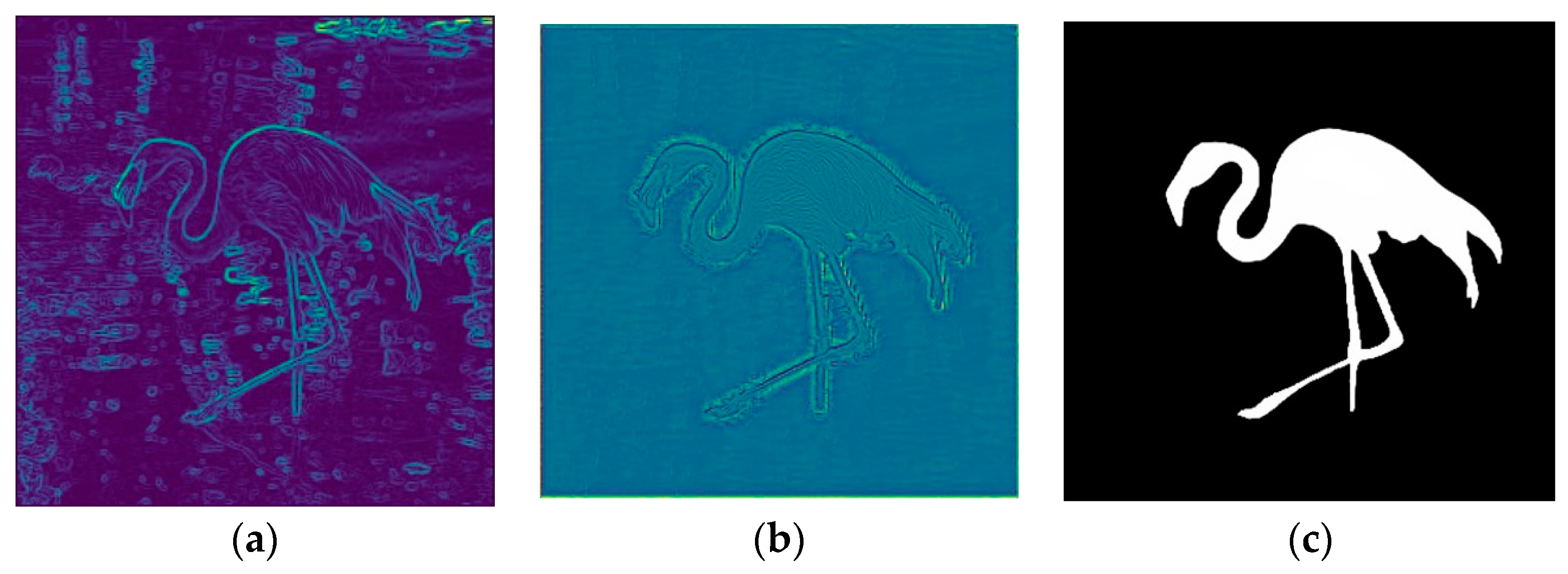
4.6. Effectiveness of the Transition Module

The transition module acts as the bridge between the coarse map and the original image gradient. The qualitative result is shown in Figure 5, in which the Sobel operator returns all of the boundaries of the objects in Figure 5a. In addition, the transition module is able to adapt the coarse map, and reject many unrelated boundaries as in Figure 5b. This feature is later utilized by the refinement module to generate the final prediction as in Figure 5c, in which it produces an accurate boundary for the saliency result.

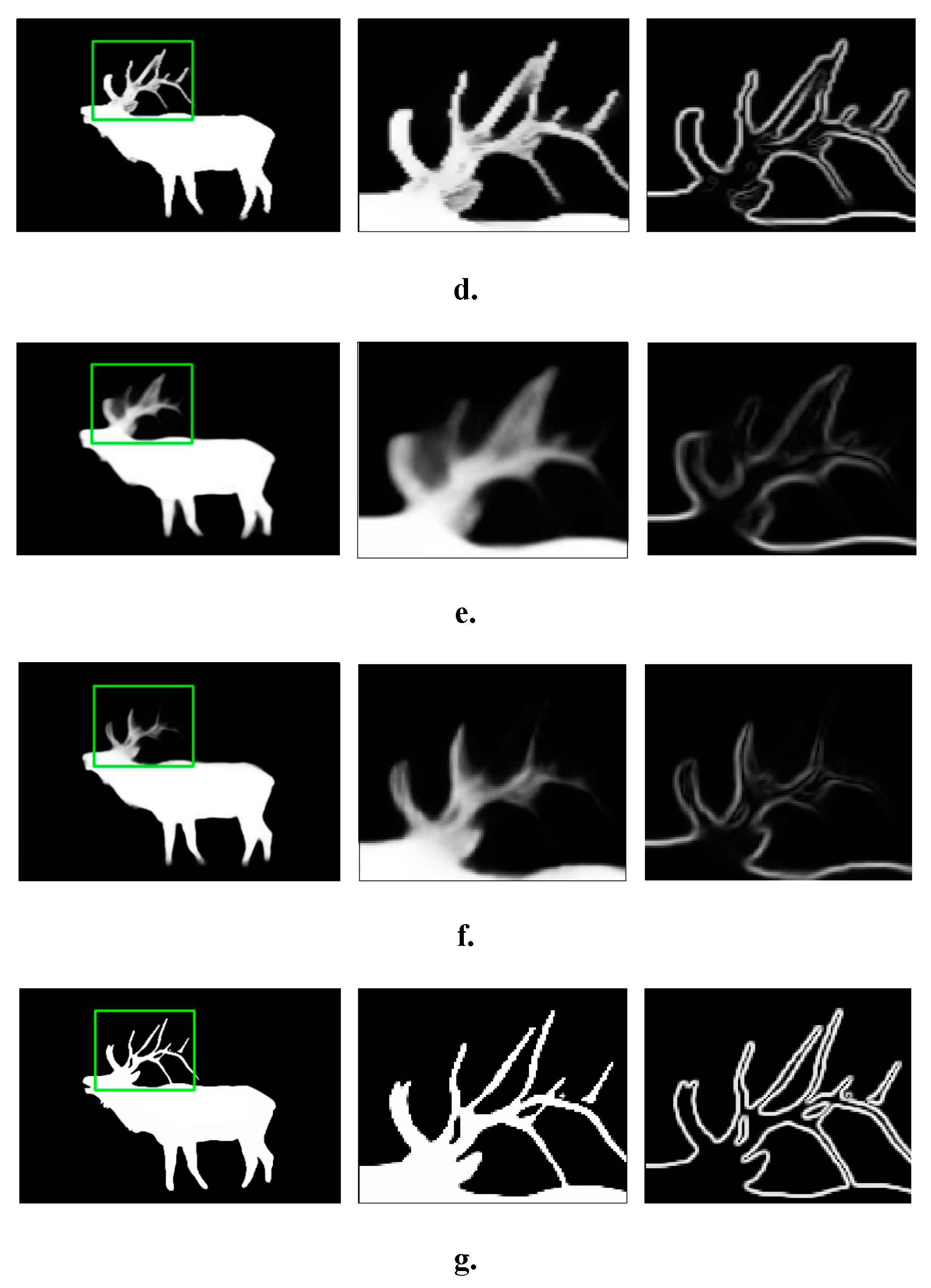
4.7. Qualitative and Quantitative Result

Table 2. Comparison with former schemes. The records highlighted in green, blue and red colors indicate first, second and third best.

Method	ECSSD		DUT-OMRON		HKU-IS		DUTS-TE
	Max-F	MAE	Max-F	MAE	Max-F	MAE	Max-F	MAE
Proposed	0.943	0.035	0.843	0.051	0.928	0.030	0.865	0.042
MLMSNet [19]	0.914	0.038	0.742	0.056	0.893	0.034	0.802	0.045
CPD-RA [20]	0.934	0.043	0.783	0.059	0.918	0.038	0.852	0.048
BASNet [23]	0.942	0.037	0.805	0.056	0.928	0.032	0.860	0.047
PAGE-Net [24]	0.926	0.035	0.770	0.063	0.920	0.030	0.817	0.047
R3Net+ [25]	0.934	0.040	0.795	0.063	0.915	0.036	0.828	0.058
AFNet [32]	0.935	0.042	0.797	0.057	0.923	0.036	0.862	0.046
Iterative [33]	0.926	0.040	0.780	0.059	0.920	0.038	0.836	0.048
PiCANetR [34]	0.935	0.046	0.803	0.065	0.918	0.043	0.860	0.050
BMPM [35]	0.928	0.045	0.774	0.064	0.921	0.039	0.852	0.048
PAGRN [36]	0.927	0.061	0.771	0.071	0.918	0.048	0.854	0.055
RAS [37]	0.921	0.056	0.786	0.062	0.913	0.045	0.831	0.059
C2S [38]	0.910	0.055	0.758	0.072	0.896	0.048	0.807	0.062
RADF+ [39]	0.923	0.049	0.791	0.061	0.914	0.039	0.821	0.061
DGRL [40]	0.925	0.042	0.779	0.063	0.913	0.037	0.834	0.051
LFR [41]	0.911	0.052	0.740	0.103	0.911	0.040	0.778	0.083
SRM [42]	0.917	0.054	0.769	0.069	0.906	0.046	0.826	0.058
Amulet [43]	0.915	0.059	0.743	0.098	0.897	0.051	0.778	0.084
DSS+ [44]	0.921	0.052	0.781	0.063	0.916	0.040	0.825	0.056
NLDF+ [45]	0.905	0.063	0.753	0.080	0.902	0.048	0.813	0.065
UCF [46]	0.903	0.069	0.730	0.120	0.888	0.062	0.773	0.112
MDF [47]	0.832	0.105	0.694	0.092	0.860	0.129	0.729	0.099

shows the quantitative comparison, in which the proposed method outperforms the former schemes in terms of the Max.F and MAE. Some qualitative results are provided in Figure 6. The proposed method produces more accurate boundaries, compared with the former schemes. Some false positives are also rejected in the prediction as in the first row of Figure 6. Notably, the false negatives are also reduced compared to the BASNet as shown in the second row of Figure 6. The proposed method can also provide promising results on the details as shown in the last row of Figure 6, where the bird’s leg is well preserved compared with BASNet and RAS. Notably, during the training phase, the designed transition and refinement modules are able to facilitate a quick convergence and generate promising results. Finally the boundary quality comparison is shown in Figure 7.

5. Conclusions

In this study, a novel salient object detection scheme was proposed to solve the bottleneck prediction scheme, and reduce computation by reducing the image size for initial prediction. The proposed MEAN network performs well in prediction and refinement. The proposed refinement strategy adopts image gradient as the refinement guidance, and it can maintain the stability of the prediction across various scales. Experimental results demonstrate that the performance is improved by resizing the coarse map into its original image size, and subsequently refining the coarse map. By adopting the 3D CNN as a channel analyzer can facilitate the transition module to identify a better edge for the next refinement step. The proposed training mechanism for transition and refinement modules has shown good performance to generate a robust result for various refinement scenarios compared to that of the former schemes.

This study proposes some fields which can be explored in the future. The first possible improvement is on the training mechanism with an adaptive hyper-parameter. This mechanism refers to an additional module for training that can adaptively change the hyper-parameter of loss for weighting of the side-output and the refinement. By treating each loss separately, the method may achieve better performance. Another possible improvement could be automatic refinement switching. This improvement is related to choosing different refinement strategies such as BR, SQR and SKR, which depend on the need for computation. Moreover, a new architecture design for different modules can be explored further for different applications.