Improved Boundary Support Vector Clustering with Self-Adaption Support

Abstract

Concerning the good description of arbitrarily shaped clusters, collecting accurate support vectors (SVs) is critical yet resource-consuming for support vector clustering (SVC). Even though SVs can be extracted from the boundaries for efficiency, boundary patterns with too much noise and inappropriate parameter settings, such as the kernel width, also confuse the connectivity analysis. Thus, we propose an improved boundary SVC (IBSVC) with self-adaption support for reasonable boundaries and comfortable parameters. The first self-adaption is in the movable edge selection (MES). By introducing a divide-and-conquer strategy with the k-means++ support, it collects local, informative, and reasonable edges for the minimal hypersphere construction while rejecting pseudo-borders and outliers. Rather than the execution of model learning with repetitive training and evaluation, we fuse the second self-adaption with the flexible parameter selection (FPS) for direct model construction. FPS automatically selects the kernel width to meet a conformity constraint, which is defined by measuring the difference between the data description drawn by the model and the actual pattern. Finally, IBSVC adopts a convex decomposition-based strategy to finish cluster checking and labeling even though there is no prior knowledge of the cluster number. Theoretical analysis and experimental results confirm that IBSVC can discover clusters with high computational efficiency and applicability.

1. Introduction

Support vector clustering (SVC) has attracted much attention for handling clusters with arbitrary shapes [1,2]. For a better description, support vectors (SVs) with their specific coefficients should generally be collected through excellent model training, which requires a large number of valid training samples and a complex iterative analysis under specific metrics. Due to the increasing data size and weak representative samples, pricey storage and computation in the training phase frequently degrade the SVC’s performance. Meanwhile, the connectivity analysis can also be confused by inappropriate parameter settings even with the use of correct SVs. Intuitively, we expect an efficient model to be trained on fewer yet representative samples and comfortable parameters to be found at a minimal cost.

Let $\mathcal{X}$ be a data set with N data samples $\{{\mathbf{x}}_1,{\mathbf{x}}_2,\cdots ,{\mathbf{x}}_N\}$, where ${\mathbf{x}}_i\in {\mathbb{R}}^d(i\in [1,N])$ in the data space. Model training is pricey because it generally has to solve a quadratic programming problem in terms of iterative analysis on an $N\times N$ kernel matrix. Its runtime usually ranges from $O\left(N^2\right)$ to $O\left(N^3\right)$ depending on the specific case [1,3,4]. Furthermore, the number of iterative analyses is uncertain, although a great value for the final coefficient vector $\beta$ that exacerbates the practical time-cost is expected. To achieve an improvement, on the one hand, selecting the most representative subset of $\mathcal{X}$ is critical and apparent. However, few research works in the literature focus on the subset’s representativeness or purity. They frequently prefer a subset selected under a random or fixed strategy for convenience. For instance, [5] unstably partitioned $\mathcal{X}$ into k subsets for local training and global merging, while [6] set a sample rate $\theta$ to control the randomly selected data samples ($N_{\mathrm{tr}}=\theta N$) in model training and in generating Voronoi cells. Despite running fast, they resulted in an extremely unstable accuracy. Later, refs. [7,8] adopted the boundary samples to reformulate the dual problem. Even though they achieved stable performance, a large N slowed down the efficiency of boundary selection, and it suffered from noise in the cluster description and connectivity analysis. On the other hand, parameter selection stops model training at the right time for cluster discovery. In the literature [1,9], the expected cluster number k is still the most common stop condition before obtaining the appropriate kernel width q by an incremental test. However, k is what we need for discovery in practical situations [8,10]. Despite various strategies to increase q, e.g., tangent approximation [11], they are not so effective because several complete clustering analyses are required.

In order to tackle these issues, we propose an improved boundary SVC (IBSVC) with self-adaption support for reasonable boundaries and comfortable parameters. Under a divide-and-conquer strategy, it firstly collects local edges with the k-means++ support. After removing the fake edges, the pure edges are used to reformulate the dual problem with relaxed constraints. Meanwhile, the expected iterative direction of the solver impels us to directly select an optimal q, which reduces the difference between the data description drawn by the constructed model and the actual pattern. IBSVC adopts a coefficient initialization-based iteration control method and a convex decomposition-based labeling strategy for the further benefit of efficiency. The main contributions of this work lie in the following:

(1)

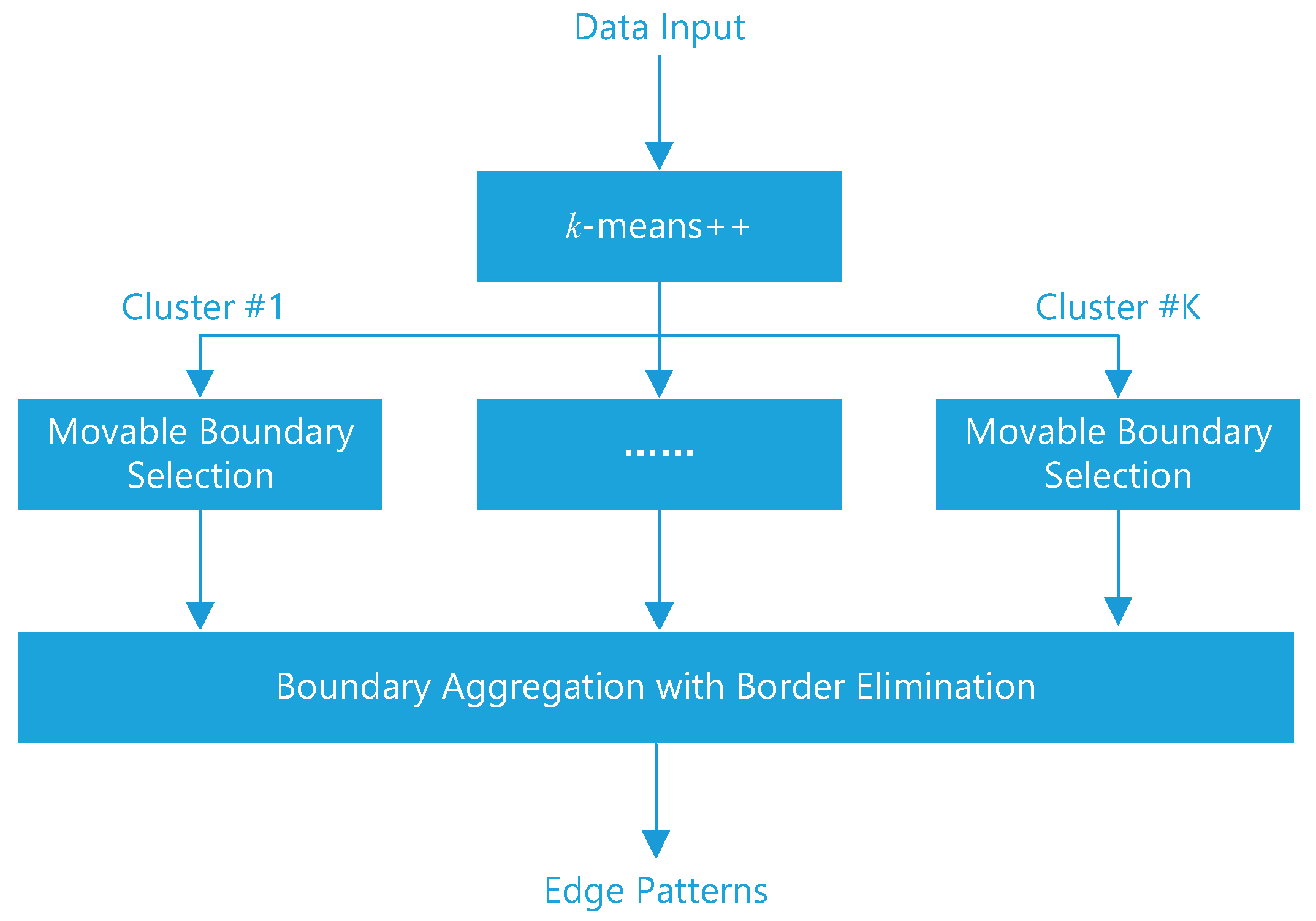
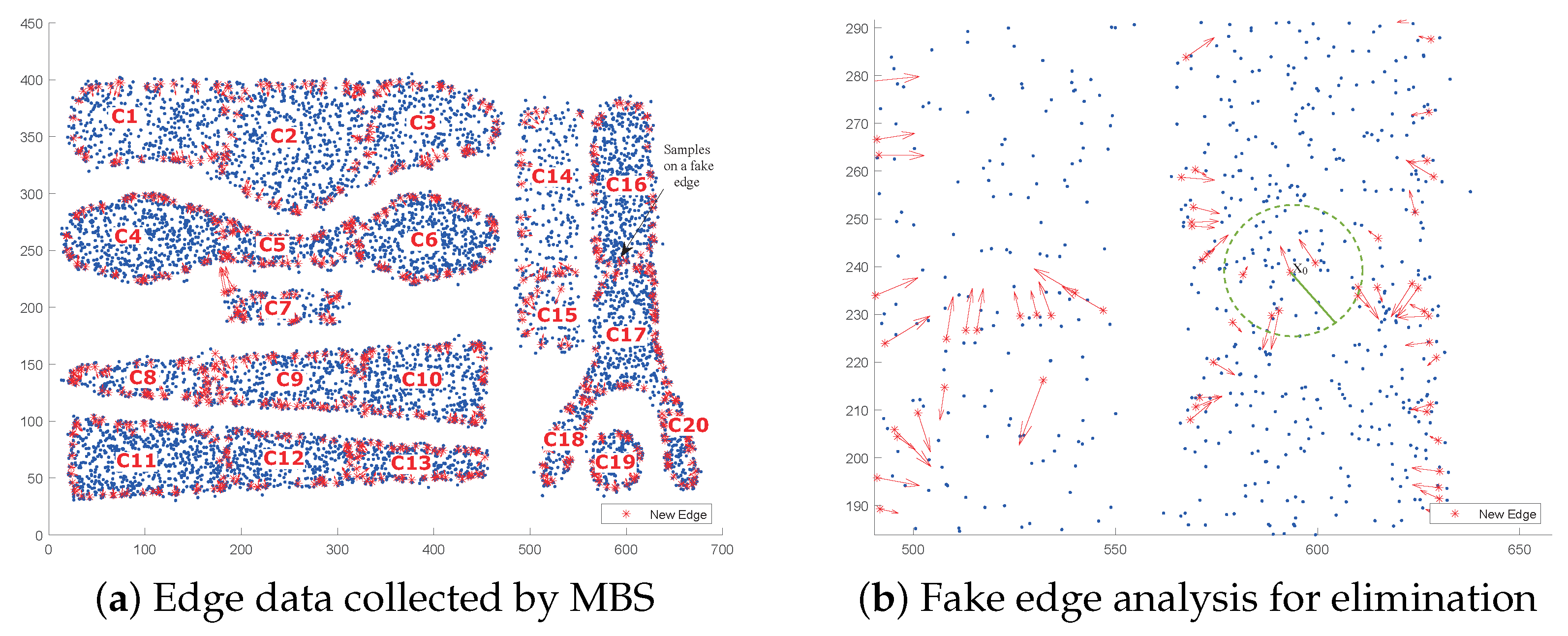
A movable edge selection (MES) method with self-adaption support is proposed. It collects local data samples from the boundaries of clusters divided by the k-means++, removes the fake edge patterns, and shrinks the remaining edges for requisite connectivity and fewer outliers. Due to the divide-and-conquer strategy, the achieved efficiency improvement enables MES to efficiently handle large-scale data analyses and supply informative and reasonable edges.

(2)

For an appropriate kernel width q, a flexible parameter selection (FPS) strategy is presented in the direct model construction without a penalty factor C. Rather than the traditional search strategy, FPS automatically adjusts q in a smaller range with a clearer target, i.e., the iterative directions drawn by the model is close to the actual data pattern. More importantly, no complete clustering procedure is required by each adjustment of q.

(3)

Benefiting from the divide-and-conquer strategy and the convex decomposition-based labeling strategy [12], IBSVC can easily adjust the discovered clusters by considering the neighborhood relationship of convex hulls even though there is no prior knowledge of the cluster number.

The remainder of this paper is organized as follows: In Section 2, both of the classic SVC and boundary SVC are briefly described. In Section 3, we first present the two self-adaption supported methods, MES and FPS, and then describe the framework of the IBSVC. After the introduction of a typical labeling phase, the theoretical analysis and experimental results of the IBSVC are presented in Section 4. Then, we give our review of related works in Section 5. Finally, conclusions are drawn in the last section, and future works to be investigated are discussed.

2. Preliminaries

2.1. Classical SVC

2.1.1. Estimation of a Trained Support Function

$\mathcal{X}$ can be mapped to a high-dimensional feature space from the data space through a nonlinear function $\Phi (·)$. Then, SVC tries to find a sphere with the minimal radius that contains most of the mapped data samples. This sphere, when mapped back to the data space, can be partitioned into several components, with each one enclosing an isolated cluster of samples. In mathematical formulation, the spherical radius R is subjected to the following:

$$\begin{array}{cc}\hfill & \underset{R,\alpha ,{\xi }_i}{min}{R}^2+C\sum _i{\xi }_i\hfill \\ \hfill & \mathrm{s}.\mathrm{t}.\left|\right|\Phi \left({\mathbf{x}}_i\right)-\alpha {\left|\right|}^2\le R^2+{\xi }_i,\hfill \end{array}$$

(1)

where $\alpha$ is the center of the sphere, ${\xi }_i$ is a slack variable, and C is a constant controlling the penalty of noise. Following [13,14], the expected sphere is estimated by a support function, which is defined as a positive scalar function $f:{\mathbb{R}}^n\to {\mathbb{R}}^{+}$. Since the support function is constructed by SVs, we estimate it by solving a dual problem in Equation (2), where ${\mathbf{x}}_i$ corresponds to the coefficient ${\beta }_i(i=1,\cdots ,N)$ if its $0<{\beta }_i<C$ is an SV.

$$\begin{array}{cc}\hfill & \underset{{\beta }_j}{max}\sum _{j}K({\mathbf{x}}_j,{\mathbf{x}}_j){\beta }_j-\sum _{i,j}{\beta }_i{\beta }_{j}K({\mathbf{x}}_i,{\mathbf{x}}_j)\hfill \\ \hfill & \mathrm{s}.\mathrm{t}.\sum _j{\beta }_j=1,0\le {\beta }_j\le C,j=1,\cdots ,N.\hfill \end{array}$$

(2)

By optimizing Equation (2) with a Gaussian kernel $K({\mathbf{x}}_i,{\mathbf{x}}_j)=e^{-q\left|\right|{\mathbf{x}}_i-{\mathbf{x}}_j{\left|\right|}^2}$, the trained objective support function can be formulated by the squared radial distance of the image of $\mathbf{x}$ from the sphere center $\alpha$ given by the following equation:

$$f\left(\mathbf{x}\right)=1-2\sum _j{\beta }_{j}K({\mathbf{x}}_j,\mathbf{x})+\sum _{i,j}{\beta }_i{\beta }_{j}K({\mathbf{x}}_i,{\mathbf{x}}_j).$$

(3)

$$\alpha =\sum _j{\beta }_j\Phi \left({\mathbf{x}}_j\right).$$

(4)

Theoretically, the radius R is usually defined by the square root of $f\left({\mathbf{x}}_i\right)$, where ${\mathbf{x}}_i$ is any one of the SVs.

2.1.2. Cluster Assignments

Since SVs are located on the border of clusters, a simple graphical connected component method can be used for cluster labeling. For any two samples, ${\mathbf{x}}_i$ and ${\mathbf{x}}_j$, we check the m segmers on the line segment connecting them by allowing their images to travel in the hypersphere. According to Equation (3), ${\mathbf{x}}_i$ and ${\mathbf{x}}_j$ should be labeled with the same cluster index, while all the m segmers always lie in the hypersphere, i.e., $f\left({\mathbf{x}}_{\tilde{m}}\right)\le R^2$ for $\tilde{m}\in [1,m]$. Otherwise, they will be in two different clusters.

2.2. Boundary SVC

In geometry, a cluster boundary consists of edge and border patterns. A cluster has independent edge patterns, while any two clusters with overlapping regions share the same border patterns. We usually consider them as two cluster components for the latter unless they have different labels. Following the support vector data description (SVDD), edge patterns are critical for the description of a cluster in unsupervised learning. Edge patterns should be the most informative samples that can accurately describe the data distribution structure without border patterns. Taken from another perspective, they can be considered as the superset of the SVs. Therefore, ref [8] proposed a classic boundary SVC (BSVC) which constructs a support function equivalent to (3), directly using the boundaries ${\mathcal{X}}_{\mathrm{b}}=\{{\mathbf{x}}_{{\mathrm{b}}_1},{\mathbf{x}}_{{\mathrm{b}}_2},\cdots ,{\mathbf{x}}_{{\mathrm{b}}_M}\}\subseteq \mathcal{X}$.

In theory, $f\left({\mathbf{x}}_{{\mathrm{b}}_i}\right)$ ($i=1,2,\cdots ,M$) should be approximately equal. Hence, we have the following equation:

$$\left\{\begin{array}{c}\sum _j{\beta }_j[K({\mathbf{x}}_{{\mathrm{b}}_j},{\mathbf{x}}_{{\mathrm{b}}_1})-K({\mathbf{x}}_{{\mathrm{b}}_j},{\mathbf{x}}_{{\mathrm{b}}_2})]\le {\xi }_1,\hfill \\ \sum _j{\beta }_j[K({\mathbf{x}}_{{\mathrm{b}}_j},{\mathbf{x}}_{{\mathrm{b}}_1})-K({\mathbf{x}}_{{\mathrm{b}}_j},{\mathbf{x}}_{{\mathrm{b}}_3})]\le {\xi }_2,\hfill \\ \cdots \hfill \\ \sum _j{\beta }_j[K({\mathbf{x}}_{{\mathrm{b}}_j},{\mathbf{x}}_{{\mathrm{b}}_1})-K({\mathbf{x}}_{{\mathrm{b}}_j},{\mathbf{x}}_{{\mathrm{b}}_M})]\le {\xi }_{M-1},\hfill \end{array}\right.$$

(5)

where $j=1,2,\cdots ,M$ and ${\sum }_j{\beta }_j=1$. Let $\beta ={[{\beta }_1,{\beta }_2,\cdots ,{\beta }_M]}^T$, $\xi ={[{\xi }_1,{\xi }_2,\cdots ,{\xi }_{M-1}]}^T$, and $\mathit{Q}={[Q_1,Q_2,\cdots ,Q_{M-1}]}^T$, where:

$$\begin{array}{cc}\hfill Q_t=[1-K({\mathbf{x}}_{{\mathrm{b}}_1},& {\mathbf{x}}_{{\mathrm{b}}_{t+1}}),K({\mathbf{x}}_{{\mathrm{b}}_2},{\mathbf{x}}_{{\mathrm{b}}_1})-K({\mathbf{x}}_{{\mathrm{b}}_2},{\mathbf{x}}_{{\mathrm{b}}_{t+1}}),\hfill \\ \hfill & \cdots ,K({\mathbf{x}}_{{\mathrm{b}}_M},{\mathbf{x}}_{{\mathrm{b}}_1})-K({\mathbf{x}}_{{\mathrm{b}}_M},{\mathbf{x}}_{{\mathrm{b}}_{t+1}})],\hfill \end{array}$$

(6)

and $t=1,2,\cdots ,M-1$. Thus, we have $\mathit{Q}\beta \le \xi$, whose objective can be approximated by the equation below:

$$\begin{array}{cc}\hfill & \underset{\beta }{min}{\beta }^T\mathit{H}\beta \hfill \\ \hfill \mathrm{s}.\mathrm{t}.& \sum _j{\beta }_j=1,\forall j\in [1,M],{\beta }_j\ge 0\hfill \end{array}$$

(7)

where $\mathit{H}={\mathit{Q}}^T\mathit{Q}$ is a Hessian matrix in ${\mathbb{R}}^{M\times M}$. Notice that (7) is a standard convex quadratic program. Using the boundaries, it replaces (2) to estimate a trained support function for BSVC. Furthermore, BSVC is compatible with the state-of-the-art strategy for cluster assignments.

3. The Proposed IBSVC

3.1. Movable Edge Selection

Regarding cluster boundary collection, Li and Maguire [15] designed a border-edge pattern selection (BEPS) algorithm. Although its contributions to clustering and classification have been confirmed, the double loop of a distance analysis between all the data sample pairs requires a pricey computation. Moreover, BEPS frequently suffers from noise along with un-shrunk edges [8]. Therefore, we propose the MES method, a hybrid framework of the k-means++ and BEPS, with an easy shrinking strategy and a fake edge removal strategy. The framework of MES is depicted in Figure 1.

Following the classic divide-and-conquer strategy, MES utilizes k-means++ to divide the data set into a number of clusters. As an optional phase, it is strongly recommended for large-scale data. Due to the shortcomings of the circle-like pattern hypothesis and the fact that the cluster number K is unknown, the obtained clusters frequently cannot reflect the ground truth of data distribution well. Thus, a movable boundary selection (MBS) with an easy shrinking strategy is first designed to collect cluster boundaries while eliminating as much noise as possible. As for better supporting arbitrary shapes, the fake edge removal strategy is integrated into the boundary aggregation with border elimination.

3.1.1. Movable Boundary Selection

On five Gaussians [5], we conducted a comparative analysis in Figure 2 before presenting the algorithm description of MBS. As discussed in Section 4 of [8], BEPS cannot obtain the shrunken edges that frequently reserve too many data samples located in the outermost section of the clusters. Due to the poor data description, as shown in Figure 2a, these data can be considered as noise or outliers. Thus, in [8], a shrinkable boundary selection (SBS) method was presented to avoid most of the noise by introducing an upper bound. However, according to Figure 2b, we can still find data samples disturbing the form of clear clusters that might affect the further use of edges. Do we have to use a subset of the input data to represent the edges for a description of the arbitrary shapes of clusters? Apparently, similar to [7] finding boundaries to replace the SVs, we can also use any equivalent edges to reach the same objective.

Taking the norm vector as the convergence direction, following [15], it is clear that the outermost data samples have bigger modules than the others close to the cluster center (see Figure 2c). Therefore, to smooth the edges, the proposed easy shrinking strategy is quite simple: move the selected outermost data towards the corresponding cluster centers. Intuitively, the step length for each movement should reflect its specific location. In Algorithm 1, we formulate this movement with the following equation:

$${\mathbf{x}}_i^{\prime }={\mathbf{x}}_i+{\tau }_{\mathrm{b}}·{\mathbf{n}}_i.$$

(8)

Here, ${\mathbf{n}}_i$ is the convergence direction of ${\mathbf{x}}_i$, and ${\tau }_{\mathrm{b}}$ is a speed factor for the movement, with a recommended range of $(0,1]$. After this movement, the obtained edges by MBS will be new data samples that are not in $\mathcal{X}$. Thus, according to lines 13–17, their convergence directions should be changed in accordance with the new neighbor relationship. Figure 2d depicts a special example with ${\tau }_{\mathrm{b}}=1$.

Algorithm 1 Movable Boundary Selection

Require: Dataset ${\mathcal{X}}_k$, thresholds ${\gamma }_l,{\gamma }_u,{\tau }_{\mathrm{b}}$, integer $k_1$ Ensure: Original edges ${\mathcal{X}}_{\mathrm{e}k}$ and normal vectors ${\mathcal{V}}_{\mathrm{e}k}$; New edges ${\mathcal{X}}_{\mathrm{e}k}^{\prime }$ and normal vectors ${\mathcal{V}}_{\mathrm{e}k}^{\prime }$  1: ${\mathcal{X}}_{\mathrm{e}k}\leftarrow \varnothing$, ${\mathcal{X}}_{\mathrm{e}k}\leftarrow \varnothing$, ${\mathcal{X}}_{\mathrm{e}k}^{\prime }\leftarrow \varnothing$, ${\mathcal{X}}_{\mathrm{e}k}^{\prime }\leftarrow \varnothing$  2: for a given data sample ${\mathbf{x}}_i$ in ${\mathcal{X}}_k$ do  3:    find the $k_1$ nearest neighbors ${\mathbf{x}}_j$ of ${\mathbf{x}}_i$  4:    ${\mathbf{n}}_i\leftarrow {\sum }_{j=1}^{k_1}{\mathbf{v}}_{ji}$, where ${\mathbf{v}}_{ji}={\mathbf{x}}_j-{\mathbf{x}}_i$  5:    ${\ell }_i\leftarrow \frac{1}{k_1}{\sum }_{j=1}^{k_1}\mathrm{g}({\mathbf{n}}_i^{\mathrm{T}}·{\mathbf{v}}_{ji})$  6:    if ${\gamma }_l\le {\ell }_i\le {\gamma }_u$ then  7:      ${\mathbf{x}}_i^{\prime }={\mathbf{x}}_i+{\tau }_{\mathrm{b}}·{\mathbf{n}}_i$  8:      ${\mathcal{X}}_{\mathrm{e}k}\leftarrow {\mathcal{X}}_{\mathrm{e}k}\cup {\mathbf{x}}_i$  9:      ${\mathcal{X}}_{\mathrm{e}k}^{\prime }\leftarrow {\mathcal{X}}_{\mathrm{e}k}^{\prime }\cup {\mathbf{x}}_i^{\prime }$ 10:      ${\mathcal{V}}_{\mathrm{e}k}\leftarrow {\mathcal{V}}_{\mathrm{e}k}\cup {\mathbf{n}}_i$ 11:    end if 12: end for 13: for a given data sample ${\mathbf{x}}_{\mathrm{e}i}$ in ${\mathcal{X}}_{\mathrm{e}k}$ do 14:    find the nearest neighbor ${\mathbf{x}}_j$ of ${\mathcal{X}}_k$ 15:    ${\mathbf{n}}_{\mathrm{e}i}\leftarrow {\mathbf{n}}_j$ 16:    ${\mathcal{V}}_{\mathrm{e}k}^{\prime }\leftarrow {\mathcal{V}}_{\mathrm{e}k}^{\prime }\cup {\mathbf{n}}_{\mathrm{e}i}$ 17: end for 18: return${\mathcal{X}}_{\mathrm{e}k}$, ${\mathcal{V}}_{\mathrm{e}k}$, ${\mathcal{X}}_{\mathrm{e}k}^{\prime }$ and ${\mathcal{V}}_{\mathrm{e}k}^{\prime }$

3.1.2. Boundary Aggregation with Border Elimination

Due to the inherent defects of k-means++, irregularly shaped clusters might be split into multiple components. Based on local geometrical and statistical information, edge patterns collected by MBS can be adjacent and are assigned to different clusters. In fact, they are located in the same cluster as the irregular shapes. As depicted by Figure 3a, the Chameleon [16,17] with eight clusters is divided into ten clusters by k-means++, with $K=10$. However, the collected edge patterns give us an illusion of 20 components, i.e., $C1,C2,\cdots ,C20$. If we can eliminate those fake edge patterns connecting two adjacent components, such as the data samples connecting $C16$ and $C17$, the remaining edge patterns from different components can be aggregated to better describe the true cluster shapes. In the literature, these fake edge patterns can be likened to border patterns [15] or transition points [18]. To correctly remove them, as shown in Figure 3b, we zoom in on a local region between $C16$ and $C17$ in order to analyze the fake edge pattern.

Let ${\mathbf{x}}_0$ be the current data sample. Three out of its five nearest neighbors have convergence directions towards $C17$, while the other two converge on $C16$. Therefore, if a cluster has been divided into multiple components, the fake edge patterns are usually located at the division position. Since boundaries are independently selected from each component, the data samples at the division position can have different convergence directions. Furthermore, the closer a data sample’s corresponding cluster center is, the more balanced the number of data samples in different convergence directions will be. The balance degree of the convergence directions of a data sample’s k nearest neighbors can be formulated as follows:

$$D_{\mathrm{f}}=\frac{k}{{\sum }_{j=1}^{k}g({\mathbf{n}}_{\mathrm{e}i}^T·{\mathbf{n}}_{\mathrm{e}j})}-1,$$

(9)

where $(·)$ means inner product, and $g\left(x\right)$ returns 1 if $x\ge 0$; otherwise, it returns 0. Algorithm 2 illustrates the procedure of boundary aggregation with border elimination in which fake edge patterns are removed. All the local edges ${\mathcal{X}}_{\mathrm{e}k},{\mathcal{X}}_{\mathrm{e}k}^{\prime }(k=1,\cdots ,K)$ are aggregated into ${\mathcal{X}}_{\mathrm{e}}$ in lines 1 and 2. From a global perspective, fake edge patterns are collected based on the balance degree analysis in lines 6–9 and eliminated in line 11. Thus, the final edge patterns are globally considered to describe the clusters.

Algorithm 2 Boundary Aggregation with Border Elimination

Require: Local original edges ${\mathcal{X}}_{\mathrm{e}k}$ and normal vectors ${\mathcal{V}}_{\mathrm{e}k}(k=1,\cdots ,K)$; Local new edges ${\mathcal{X}}_{\mathrm{e}k}^{\prime }$ and normal vectors ${\mathcal{V}}_{\mathrm{e}k}^{\prime }(k=1,\cdots ,K)$, $k_2$ and ${\tau }_{\mathrm{f}}$ Ensure: Global edges ${\mathcal{X}}_{\mathrm{ge}}$ with their normal vectors ${\mathcal{V}}_{\mathrm{ge}}$  1: ${\mathcal{X}}_{\mathrm{e}}\leftarrow {\bigcup }_{k=1}^K{\mathcal{X}}_{\mathrm{e}k}$, ${\mathcal{V}}_{\mathrm{e}}\leftarrow {\bigcup }_{k=1}^K{\mathcal{V}}_{\mathrm{e}k}$  2: ${\mathcal{X}}_{\mathrm{e}}^{\prime }\leftarrow {\bigcup }_{k=1}^K{\mathcal{X}}_{\mathrm{e}k}^{\prime }$, ${\mathcal{V}}_{\mathrm{e}}^{\prime }\leftarrow {\bigcup }_{k=1}^K{\mathcal{V}}_{\mathrm{e}k}^{\prime }$  3: ${\mathcal{I}}_{\mathrm{fe}}\leftarrow \varnothing$  4: for a given data sample ${\mathbf{x}}_{\mathrm{e}i}$ in ${\mathcal{X}}_{\mathrm{e}}$ do  5:    find the $k_2$ nearest neighbors ${\mathbf{x}}_{\mathrm{e}j}$ of ${\mathbf{x}}_{\mathrm{e}i}$  6:    $D_{\mathrm{f}}\leftarrow \frac{k_2}{{\sum }_{j=1}^{k_2}g({\mathbf{n}}_{\mathrm{e}i}^T·{\mathbf{n}}_{\mathrm{e}j})}-1$  7:    if $D_{\mathrm{f}}\ge {\tau }_{\mathrm{f}}$ then  8:      ${\mathcal{I}}_{\mathrm{fe}}\leftarrow {\mathcal{I}}_{\mathrm{fe}}\cup i$  9:    end if 10: end for 11: ${\mathcal{X}}_{\mathrm{ge}}\leftarrow {\mathcal{X}}_{\mathrm{e}}^{\prime }\setminus \forall {\mathbf{x}}_{\mathrm{e}i}$, ${\mathcal{V}}_{\mathrm{ge}}\leftarrow {\mathcal{V}}_{\mathrm{e}}^{\prime }\setminus \forall {\mathbf{n}}_{\mathrm{e}i}$ where $i\in {\mathcal{I}}_{\mathrm{fe}}$  12: return ${\mathcal{X}}_{\mathrm{ge}}$, ${\mathcal{V}}_{\mathrm{ge}}$ =0

3.2. Improved Hypersphere Construction

The final edge patterns obtained by MES are generally the candidate SVs, which construct the expected minimal hypersphere with the radius R. To filter out non-SVs, BSVC reformulates Equation (7) by Equation (10) with ${\tilde{\mathit{H}}}_{ij}=2{\mathit{H}}_{ij}$, which allows $0\le {\beta }_j\le 1$ and removes fewer informative points with ${\beta }_j\le {10}^{-lgM}$.

$$\begin{array}{cc}\hfill & \underset{\beta }{min}\frac{1}{2}{\beta }^T\tilde{\mathit{H}}\beta \hfill \\ \hfill & \mathrm{s}.\mathrm{t}.0\le {\beta }_j\le 1,j=1,\cdots ,M.\hfill \end{array}$$

(10)

However, to traverse the same edge patterns, we can frequently find out distinct paths that might suggest different shapes and relationships of clusters. Generally, more optional paths exist if we allow more edge patterns to have ${\beta }_j=0$. Intuitively, more edge patterns are expected to be the final SVs in order to provide a better description of the clusters. Meanwhile, BSVs with ${\beta }_j=1$ are no longer recommended even though most of them are replaced by Equation (8). Thus, with a constraint relaxation, the dual problem (10) is further formulated by the equation below:

$$\begin{array}{cc}\hfill & \underset{\beta }{min}\frac{1}{2}{\beta }^T\tilde{\mathit{H}}\beta \hfill \\ \hfill & \mathrm{s}.\mathrm{t}.0<{\beta }_j<1,j=1,\cdots ,M.\hfill \end{array}$$

(11)

After solving problem (11), the obtained $\beta$ constructs the expected hypersphere by following Equations (3) and (4).

3.3. Improved Solver for Dual Problem

Let $\xi$ be a scalar moving towards 0, i.e., $\xi \to 0$. Following [8], the optimization process of (11) can be started from ${\beta }^0\in R^M$ and generates a sequences of vectors ${\left\{{\beta }^k\right\}}_{k=1}^{\infty }$. For each outer iteration, ${\beta }_1,{\beta }_2,\cdots ,{\beta }_M$ are updated in M inner iterations, respectively. Thus, each outer iteration generates ${\beta }^{k,i}\in R^M,i=1,2,\cdots ,M+1$. By fixing the other variable to get an updated ${\beta }^{k,i+1}$ from ${\beta }^{k,i}$, we solve the following one-variable sub-problem:

$$\begin{array}{cc}\hfill & \underset{\theta }{min}f({\beta }^{k,i}+\theta {\mathit{e}}_i)=\frac{1}{2}{\tilde{\mathit{H}}}_{ii}{\theta }^2+{\nabla }_{i}f\left({\beta }^{k,i}\right)\theta +\mathrm{constant}\hfill \\ \hfill & \mathrm{s}.\mathrm{t}.\xi \le {\beta }_i^k+\theta \le 1-\xi ,\hfill \end{array}$$

(12)

where ${\mathbf{e}}_i={[0,\cdots ,0,1,0,\cdots ,0]}^T$. Different from Equation (16) of [8], this objective function has an updated projected gradient ${\nabla }_i^{P}f\left(\beta \right)$ with new constraints:  

$${\nabla }_i^{P}f\left(\beta \right)=\left\{\begin{array}{cc}{\nabla }_{i}f\left(\beta \right)\hfill & \mathrm{if}\xi <{\beta }_i<1-\xi \hfill \\ min({\nabla }_{i}f\left(\beta \right),\xi )\hfill & \mathrm{if}{\beta }_i=\xi \hfill \\ max({\nabla }_{i}f\left(\beta \right),\xi )\hfill & \mathrm{if}{\beta }_i=1-\xi .\hfill \end{array}\right.$$

(13)

We move to the index $i+1$ without updating ${\beta }_i^{k,i}$ if ${\nabla }_i^{P}f\left({\beta }^{k,i}\right)=0$. If ${\tilde{\mathit{H}}}_{ii}>0$, the solution will be as follows:

$${\beta }_i^{k,i}=min\left(max\left({\beta }_i^{k,i}-\frac{{\nabla }_{i}f\left({\beta }^{k,i}\right)}{{\tilde{\mathit{H}}}_{ii}},\xi \right),1-\xi \right),$$

(14)

and will then continue the search in the current index.

Combining the formulas mentioned above with the analysis in [8], we can get an improved solver (iSolver) for the problem (11), which is shown in Algorithm 3. By using the iSolver, all the M items of $\beta$ will be kept in the range of $[\xi ,1-\xi ]$, which will reduce the ambiguity of the data description caused by the removal of the edge point, with ${\beta }_i=0$ or ${\beta }_i\le {10}^{-⎡lgM⎤}$. In fact, without the constraint, a certain percentage of edge points have zero coefficients. Furthermore, to reduce unnecessary iterations, in line 1, we introduce an initialization strategy for $\beta$ based on normal vectors ${\mathcal{V}}_{\mathrm{ge}}$. According to the principle of SVDD and the rules of connectivity analysis [13,17], BSVs with ${\beta }_i=C$, SVs with $0<{\beta }_i<C$, and Inners with ${\beta }_i=0$ are located outside, above, and inside the cluster boundary, respectively. These characteristics are similar to the relationship between a data sample’s location and its convergence direction, discussed in Section 3.1. Thus, following Algorithm 2, we initialize the coefficient ${\beta }_i$ of ${\mathbf{x}}_{\mathrm{e}i}$ by normalizing its normal vector’s modulus as follows:

$${\beta }_i=\frac{|{\mathbf{n}}_{\mathrm{e}i}|}{{max}_{j=1,\cdots ,M}\left|{\mathbf{n}}_{\mathrm{e}j}\right|+\xi }.$$

(15)

In Algorithm 3, line 2 adopts FPS to decide an appropriate kernel width q for the Hessian matrix $\mathit{H}$. FPS is detailed in Section 3.4. Due to the new constraints, all the global edges will be kept for the hypersphere construction. Therefore, without any adjustment, the radius R can be directly measured with a distance from any ${\mathrm{x}}_{\mathrm{e}i}(i\in [1,M])$ to the center.

Algorithm 3 iSolver for the Dual Problem (11)

Require: Global edges ${\mathcal{X}}_{\mathrm{ge}}$, normal vectors ${\mathcal{V}}_{\mathrm{ge}}$, and $\xi$ Ensure: Coefficient vector $\beta$  1: Strategically initialize each item of $\beta$ by Equation (15)  2: Kernel width q decided by FPS  3: Hessian matrix $\mathit{H}\leftarrow {\mathit{Q}}^T\mathit{Q}$ following Equation (6)  4: While $\beta$ is not the optimal  5: for$i=1,2,\cdots ,M$do  6:    ${\widehat{\beta }}_i\leftarrow {\beta }_i$  7:    $\widehat{G}=2\times {\sum }_{j=1}^N{\beta }_j{\mathit{H}}_{ji}$  8:    $G\leftarrow \widehat{G}+({\beta }_i-{\widehat{\beta }}_i)$  9:    $PG=\left\{\begin{array}{cc}G\hfill & \mathrm{if}\xi <{\beta }_i<1-\xi \hfill \\ min(G,\xi )\hfill & \mathrm{if}{\beta }_i=\xi \hfill \\ max(G,\xi )\hfill & \mathrm{if}{\beta }_i=1-\xi \hfill \end{array}\right.$ 10:    if $\left|PG\right|\ne 0$ then 11:      ${\beta }_i\leftarrow min(max({\beta }_i-\frac{1}{2}G,\xi ),1-\xi )$ 12:    end if 13: end for

3.4. Flexible Parameter Selection of Q

The kernel width q is critical for the accurate description of data patterns because different q values mean different resolutions. A greater q value generally leads to a tighter fitting with more SVs, while a smaller q value considers more connected clusters. Therefore, an exploration of the kernel width q cannot be avoided before an optimal division of data space is obtained. Ref. [1] discussed different strategies in the literature. Notice that Algorithm 3 keeps using all the edges collected by Algorithm 2 as the final SVs. Thus, we intuitively need a new strategy to optimize the parameter selection of q with the known SVs and their relative location on the corresponding boundary.

In [19], J. Lee and D. Lee proved that the support function (3) could be considered as a dynamical system. In this system, there is a stable equilibrium point (SEP) which can be reached by an optimization algorithm starting at any point, e.g., the gradient descent. To preserve the topological structure, following [20], the generalized gradient descent process can be formulated with the following equation:

$$\nabla f\left({\mathbf{x}}_i\right)=\sum _{j=1}^M\underset{\mathrm{coefficient}}{\underbrace{4q{\beta }_j^{k}K({\mathbf{x}}_j,{\mathbf{x}}_i)}}·\underset{\mathrm{vector}}{\underbrace{\left[{\mathbf{x}}_j-{\mathbf{x}}_i\right]}}.$$

(16)

Here, $4q{\beta }_j^{k}K({\mathbf{x}}_j,{\mathbf{x}}_i)$ scales $[{\mathbf{x}}_j-{\mathbf{x}}_i]$ and contributes to the final convergence direction. The convergence direction $\overrightarrow{{\mathbf{x}}_i}$ in the k-th iteration for ${\mathbf{x}}_i$ is the negative gradient of $f\left({\mathbf{x}}_i\right)$, i.e.:

$$\overrightarrow{{\mathbf{x}}_i}=-\gamma \nabla f\left({\mathbf{x}}_i\right),$$

(17)

where $\gamma$ is a constant factor. This is the fundamental of the convex decomposition strategy proposed by [21]. Furthermore, in each convex hull, SEP is the innermost point that is the closest to the center $\alpha$ (see Equation (4)) of the constructed hypersphere. Geometrically, for each ${\mathbf{x}}_i$, the vector field $\overrightarrow{{\mathbf{x}}_i}$ in (16) is orthogonal to the constructed hypersphere. On the basis of SVDD and Equation (8) of [15], $\overrightarrow{{\mathbf{x}}_i}$ plays the same role as the normal vector ${\mathbf{n}}_i$ in Equation (8). Intuitively, the core idea behind the proposed FPS is quite simple, i.e., an appropriate kernel width q improves the accumulated similarity between $\overrightarrow{{\mathbf{x}}_i}$ and ${\mathbf{n}}_i$, where $i=1,\cdots ,M$.

Thus, in theory, FPS can find out the q value by employing the following equation:

$$q\leftarrow arg\underset{q}{max}\sum _{i=1}^{M}cos({\mathbf{n}}_i,\overrightarrow{{\mathbf{x}}_i}).$$

(18)

Apparently, the gradient descent-like process starts early in Algorithm 1. For the sake of simplicity and efficiency, and in line with MBS, we recommend a randomly selected $M^{\prime }(\ll M)$ edge pattern to find a suitable q value. Based on the initialized $\beta$, FPS works in line 2 of Algorithm 3.

3.5. The Framework of IBSVC

By combining the aforementioned methods, we present the framework of IBSVC in Algorithm 4 by following a similar description to that of the classic SVC.

Even though several parameters are required, in Algorithm 4, most of them are not strongly depended upon by IBSVC, which will be discussed in Section 4. The training phase ranges from lines 1 to 6, in which lines 1–5 constitute the procedure of the MES. The k-means++ divides $\mathcal{X}$ into K subsets for an efficient edge collection in lines 2–4. Thus, we do not expect an accurate K as the prior knowledge. The MES in lines 2–4 can also be conducted in parallel. Based on the local edges ${\mathcal{X}}_{\mathrm{e}i}$ and their normal vectors ${\mathcal{V}}_{\mathrm{e}i}$ ($i=1,\cdots ,K$), BABE in line 5 obtains the global version through a combination with the fake edge removal. In line 6, the iSolver obtains the coefficient vector $\beta$ for all the global edges ${\mathcal{X}}_{\mathrm{ge}}$. This procedure is optimized by considering the edge locations and by introducing the kernel width q selection. Therefore, q is not included in the list of required parameters. Lines 7–14 step into the labeling phase. Without any constraints on the labeling strategy, we can generally choose any of the cluster prototypes for ${\mathcal{X}}_{\mathrm{R}}$ and any sampling strategy to match it for the connectivity analysis in lines 7–8. After that, line 9 decides on the labels of the chosen prototypes, which will be utilized in lines 10–13 to label all the remaining data.

Algorithm 4 Description of IBSVC

Require: Dataset $\mathcal{X}$, integers $K,k_1,k_2$, and thresholds ${\gamma }_l,{\gamma }_u,{\tau }_b,{\tau }_f,\xi$ Ensure: Clustering labels for all the data samples  1: $\{{\mathcal{X}}_1,\cdots ,{\mathcal{X}}_K\}\leftarrow k-\mathrm{means}++(\mathcal{X},K)$  2: for each${\mathcal{X}}_i(i=1,2,\cdots ,K)$do  3:    $\{{\mathcal{X}}_{\mathrm{e}i},{\mathcal{V}}_{\mathrm{e}i},{\mathcal{X}}_{\mathrm{e}i}^{\prime },{\mathcal{V}}_{\mathrm{e}i}^{\prime }\}\leftarrow$ MBS($k_1,{\gamma }_l,{\gamma }_u,{\tau }_b$)  4: end for  5: $\{{\mathcal{X}}_{\mathrm{ge}},{\mathcal{V}}_{\mathrm{ge}}\}\leftarrow$ BABE($\forall {\mathcal{X}}_{\mathrm{e}i},\forall {\mathcal{V}}_{\mathrm{e}i},\forall {\mathcal{X}}_{\mathrm{e}i}^{\prime },\forall {\mathcal{V}}_{\mathrm{e}i}^{\prime }$; $k_2,{\tau }_f$) with $i=1,\cdots ,K$  6: $\beta \leftarrow$ iSolver(${\mathcal{X}}_{\mathrm{ge}},{\mathcal{V}}_{\mathrm{ge}},\xi$)  7: $\mathcal{P}\leftarrow$ finding cluster prototypes for ${\mathcal{X}}_{\mathrm{ge}}$  8: $\mathit{A}\leftarrow$ sampling for connectivity analysis with $\mathcal{P}$  9: Labels ← finding connected components using $\mathit{A}$ 10: for each$\mathbf{x}\in \mathcal{X}\backslash {\mathcal{X}}_{\mathrm{ge}}$do 11:    inx← find the nearest prototype from $\mathbf{x}$ 12:    Labels[x] ← Labels[${\mathbf{x}}_{inx}$] 13: end for 14: return Labels

4. Performance Analysis

4.1. Complexity Analysis

As a hybrid method, IBSVC focuses on achieving an improvement in the training phase of BSVC [8] as well as on optimizing the kernel width q selection that has not been considered. In fact, besides [8], the fast and scalable SVC (FSSVC) [7] is another variant of BSVC. Meanwhile, the faster and reformulated SVC (FRSVC) [12] also employs a classic form of the dual coordinate descent method, which is one of the sources of inspiration for the proposed iSolver. In the literature, the Voronoi cell-based clustering (VCC) [6] is a typical data division method. To fairly evaluate IBSVC’s time complexity, let N be the number of samples in a data set, $N_{\mathrm{SV}}$ be the number of SVs, ℓ be the average number of iterations for each data sample to locate its corresponding local minimum via the steepest descent process [19], ${\ell }_{\mathrm{iter}}$ be the self-defined iteration number for BSVC and IBSVC, $N_c$ be the final number of convex hulls (CHs), M be the size of the selected cluster boundaries by FSSVC [7], and m be the average sample rate. $M_1$ and $M_2$ are the numbers of the final edge patterns obtained by BSVC and IBSVC, respectively. Due to different strategies of edge removal, $M_1$ and $M_2$ are not equal but are on the same scale. Even though the collected edges and the way the problem is constructed frequently influence the labeling performance, we focus on efficient training and refer to [8] for the baseline of the labeling phases.

In the training phase, the employed k-means++ [22] consumes $O\left(NK\right)$. Since each subset ${\mathcal{X}}_i$ has $\frac{N}{K}$ data samples, the proposed MES requires $O({\left(\frac{N}{K}\right)}^2)$. Then, BABE requires $O\left(k_2{M}_2\right)$ to remove the fake edges, while the iSolver takes $O\left(M_2^2\right)$ to get $\beta$ for the support vector function in Equation (3). Therefore, the total time complexity for the training phase of IBSVC is $O(NK+{\left(\frac{N}{K}\right)}^2+k_2{M}_2+M_2^2)$. Generally, we have $K\ll N$ and $k_2\ll M_2$. Thus, this complexity can be simplified by $O({\left(\frac{N}{K}\right)}^2+M_2^2)$. By contrast, BSVC consumes $O(N^2+M_1^2)$. Both of them are much lower than the $O\left(N^3\right)$ required by the conventional methods [1]. For the labeling phase, both IBSVC and BSVC adopt the construction of CHs and the performance of connectivity analyses between them. The prior decomposition respectively uses self-defined ${\ell }_{\mathrm{iter}}$ iterations from the $M_2$ and $M_1$ data samples. The latter analysis is flexible to any sampling strategy based on CHs, e.g., the strategy from the FSSVC or the faster and reformulated SVC (FRSVC) [12]. Thus, we denote it with a linear function $f\left(\zeta \right)$, where $\zeta$ can be either $N_c$ or $N_{\mathrm{SV}}$.

We compare IBSVC with the state-of-the-art methods, i.e., FRSVC [12], FSSVC [7], Voronoi cell-based clustering (VCC) [6], fast support vector clustering (FSVC) [5], and the reformative SVC with elementary operations (RSVC-EO) [20]. In addition, we consider k-means++ as one of the baselines for it is a classic clustering method and plays an important role in IBSVC. In

Table 1. Time complexity analysis of the state-of-the art methods.

Index	Method	SVC Training	Labeling
1	FSVC	$O\left(N^3\right)$	$O(\ell N_b+\gamma N^2)$
2	VCC	$O\left(N_{tr}^3\right)$	Mode I: $O(\ell N_{tr}+m{N}_c^2)$
			Mode II: $O(\ell N_b+\gamma N_{tr}^2+m{N}_b^2)$
3	FSSVC	$O(N^2+M^3)$	$O(\ell N_{\mathrm{SV}}+2m{N}_c)$ or $O\left(N_{\mathrm{SV}}^2\right)$
4	FRSVC	$O\left(\tilde{d}{N}^2\right)$	$O(\ell N_{\mathrm{SV}}+\overline{m}{N}_c)$
5	RSVC-EO	$O\left(\tilde{d}{N}^2\right)$	$O(N_{\mathrm{SV}}^2+\rho N_{\mathrm{CH}}+N{N}_{\mathrm{SV}})$
6	BSVC	$O(N^2+M_1^2)$	$O({\ell }_{\mathrm{iter}}{M}_1+f\left(\zeta \right))$
7	IBSVC	$O({\left(\frac{N}{K}\right)}^2+M_2^2)$	$O({\ell }_{\mathrm{iter}}{M}_2+f\left(\zeta \right))$
8	k-means++	$O\left(NK\right)$

Note: $\tilde{d}\in \left[1\le \tilde{d}\le d\right], \overline{m}\in (1,2], \rho \in (2,3], N_{tr}=\theta N with \theta \in (0,1]$.

, $\gamma$ ranges from $1/N$ to 1, $N_{tr}$ is the number of data that is uniformly sampled with a predefined sample rate $\theta$, and $N_b$ is the number of small balls extracted, either from the $N_{tr}$ data samples for VCC or from the whole data set for the others. Even though two optional modes of the labeling phase are presented for VCC, in this study, Mode I, which has a fast phase for labeling the remaining data, is preferred for its relative stability. Even though FRSVC and RSVC-EO have solvers that are similar to BSVC, their problems and data forms are different. A large N makes FRSVC and RSVC-EO adopt calculation on demand, which takes $O\left(d{N}^2\right)$; in this case, d is the data dimension. Therefore, their time complexities in the training phase should be $O\left(\tilde{d}{N}^2\right)$, with $1\le \tilde{d}\le d$. The difference is in the labeling phases, where the RSVC-EO performs non-iteration convex decomposition and a connectivity analysis irrespective of the sampling separately costing $O\left(N_{\mathrm{SV}}^2\right)$ and $O\left(\rho N_{\mathrm{CH}}\right)$ ($\rho \in (2,3]$). For all the methods, labeling the remaining data sample is omitted since the time complexity is linear to $N_c$ or $N_{\mathrm{SV}}$.

4.2. Datasets and Experimental Settings

Derived from the BSVC [8], the proposed IBSVC adopts at least three distinct ways for improvements, i.e., a k-means++ based MES to support large-scale data, the iSolver with optimal constraints for ambiguity reduction in SVDD, and the FPS for a direct kernel width search without complete clustering procedure attempts. To achieve a full performance analysis, we conduct the following five experiments:

(1)

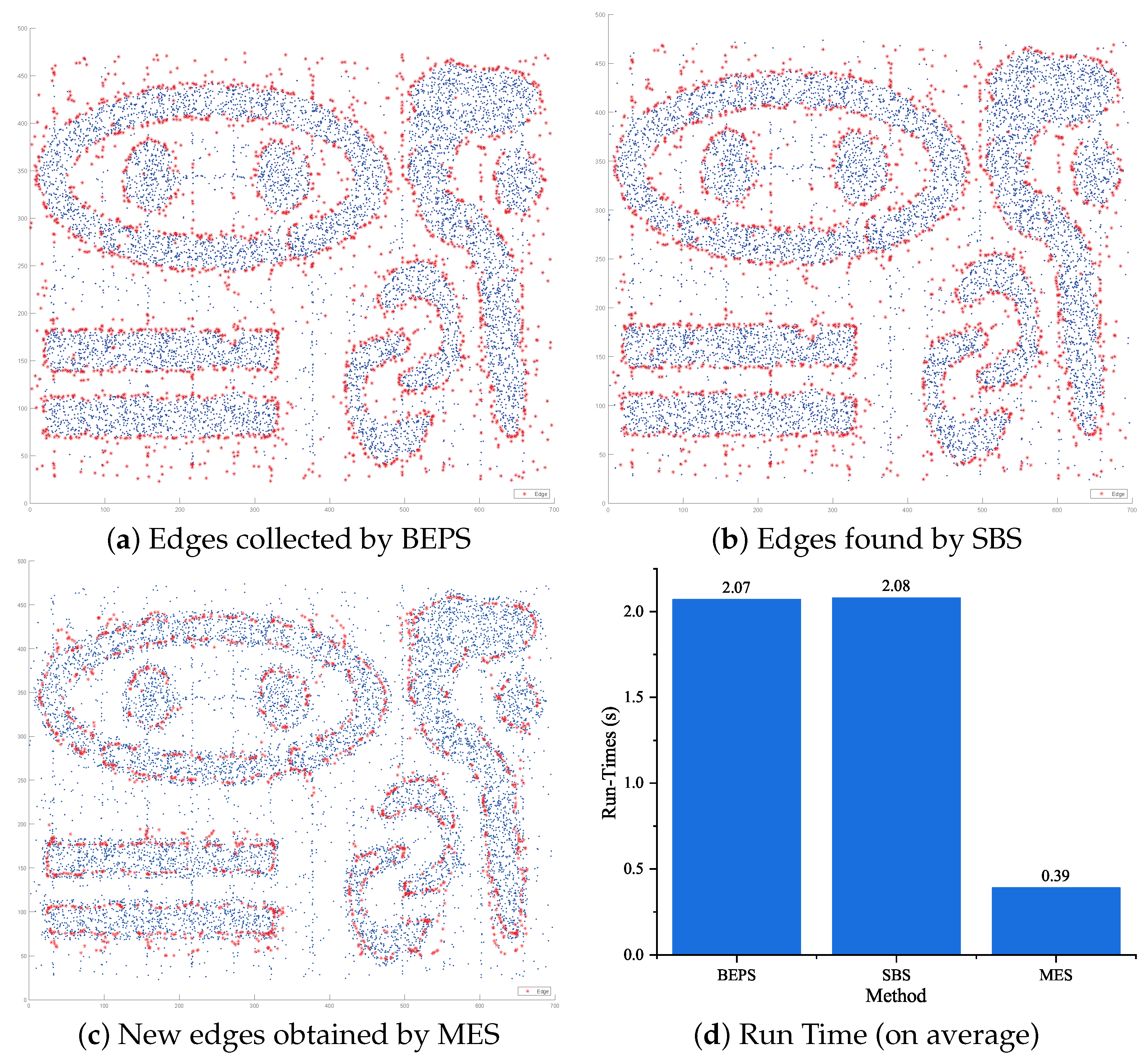
Check whether the MES correctly and efficiently obtains informative edges for data description.

(2)

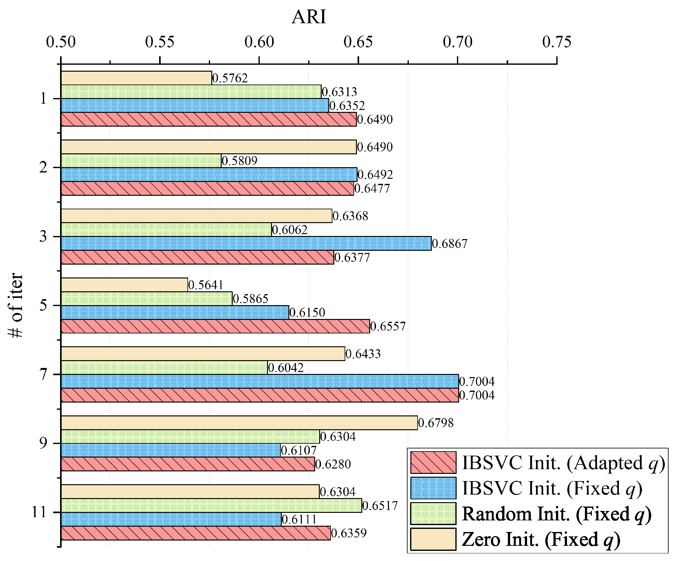
Find out how the $\beta$ initialization strategy affects the number of iterations required by the iSolver and whether the effect can be maintained if we limit the iteration number to a small one, such as with the BSVC.

(3)

Make several comparisons between the FPS and the traditional strategy to collect evidence corresponding to its efficiency and usability. The former is about the run-time, while the latter is closely related to the gap between the discovered kernel width q and the ideal value.

(4)

Perform a comprehensive analysis of the IBSVC based on its comparison with the state-of-the-art variants of the SVC listed in Table 1, which adopt a method similar to clustering.

(5)

Compare IBSVC with the typical k-means++ [22] to verify the cost–performance ratio since k-means++ is well-known for its efficiency.

The aforementioned experiments are conducted on typical data sets from various domains: Synthetic Chameleon is a noise-eliminated version of DS 4 from [16]. A breast cancer dataset called wisconsin and imbalanced shuttle data are provided by the UCI repository [23]. One classic text corpora known as 20Newsgroups [24], with twenty full categories, were processed by [25] following the method of ${\mathrm{DC}}_{\mathrm{GLI}}-\mathrm{CCE}$. UNIBS Anonymized 2009 Internet Traces UNIBS-AIT [26] consists of 9209 flows in four imbalance-distributed categories, i.e., WEB (HTTP and HTTPS), MAIL (POP2, IMAP as well as their encrypted flows), BitTorrent, and eMule. It was supplied by TNG@UniBS Lab and processed by [27] for early traffic behavior analysis. Following the work of [28], kddcup99 is a nine-dimensional data set extracted from the KDD Cup 1999 Data [29], which was used to build a network intrusion detector. The statistical information of the sixteen employed data sets are listed in

Table 2. Description of the benchmark data sets.

Data Sets	Data Set Description
	Size	Dims	# of Classes
wisconsin	683	9	2
Chameleon	7670	2	8
UNIBS-AIT	9209	4	4
20Newsgroups	13,998	20	20
shuttle	43,500	9	7
kddcup99	494,021	9	5

.

To evaluate the accuracy, we adopted the widely used similarity metrics known as the adjusted rand index (ARI) [30], formulated by Equation (19). In Equation (19), $N_{ij}$ is the number of data points with a true label i but is labeled with j, while $N_{i·}$ and $N_{·j}$ are the number of data points with the labels i and j, respectively.

$$\mathrm{ARI}=\frac{{\sum }_{i,j}\left(\genfrac{}{}{0pt}{}{N_{ij}}{2}\right)-\left[{\sum }_i\left(\genfrac{}{}{0pt}{}{N_{i·}}{2}\right){\sum }_j\left(\genfrac{}{}{0pt}{}{N_{·j}}{2}\right)\right]/\left(\genfrac{}{}{0pt}{}{N}{2}\right)}{\frac{1}{2}\left[{\sum }_i\left(\genfrac{}{}{0pt}{}{N_{i·}}{2}\right)+{\sum }_j\left(\genfrac{}{}{0pt}{}{N_{·j}}{2}\right)\right]-\left[{\sum }_i\left(\genfrac{}{}{0pt}{}{N_{i·}}{2}\right){\sum }_j\left(\genfrac{}{}{0pt}{}{N_{·j}}{2}\right)\right]/\left(\genfrac{}{}{0pt}{}{N}{2}\right)}$$

(19)

In this study, we implemented the IBSVC and all the compared methods in MATLAB 2021b without the use of any parallelization tricks. As with the previous settings, the flexibility and usability of the proposed IBSVC prompted the most amount of concern in this study. Efficiency improvement is a matter of course. Therefore, the employed testbed is a computer running Windows 10-X64 on Intel I7-10700@2.90 GHz and 16 GB RAM. For fair comparisons, the run-time cost for each data set is an average of ten times that of the execution.

4.3. Performance of MES for Informative Edges

MES is a hybrid method that consists of three critical components, i.e., k-means++, MBS, and BABE. Compared with BEPS [15], theoretically, MES shrinks the cluster boundary by restricting the upper bound ${\gamma }_u<1$. Thus, noise interference is weak since a proportion of outliers is separated. Based on BSVC, MES supports data division, data movements, and the generation of more informative edge patterns. To check whether MES correctly and efficiently obtains informative edge patterns, we utilized an additional synthetic data DS3 from [16] as a representative. The selected edge patterns and run-time cost on average are depicted in Figure 4.

Intuitively, irregular cluster shapes of DS3 are captured well by all the three methods, and the difference is that they keep different proportions of the noise data. The number of remaining noises have an apparent sequence of $N_{\mathrm{BEPS}}>N_{\mathrm{SBS}}>N_{\mathrm{MES}}$. From an SVDD perspective, these noise samples are generally recognized as outliers or bound support vectors (BSVs), which contribute to the formulation of the support vector function (3) for ${\beta }_j$ approximating 1; they affect the connectivity analysis among clusters, especially for high-dimensional data. Therefore, many data preprocessing methods in the literature have been designed and introduced before clustering. Comparatively, as shown in Figure 4c, MES removed most of the noise samples while keeping relatively clear boundaries (without borders). It is worth mentioning that the average run-time cost of 0.39 s by MES, as can be seen in Figure 4d, is far less than the 2.07 s and 2.08 s consumed by BEPS and SBS of BSVC, respectively.

4.4. Validity Analysis of the Coefficient Vector Initialization Strategy

Generally, different coefficient vector $\beta$ initialization strategies directly influence the iterative analysis of a solver. For the proposed iSolver, the $\beta$ initialization strategy is also related to the decision concerning the kernel width q. Therefore, the chosen strategy indirectly impacts the final accuracy and when the iteration should be stopped. Traditionally, zero and random initialization strategies are frequently preferred, which respectively start the solver by setting ${\beta }_j=0$ and $0<{\beta }_j<1$ for $j=1,\cdots ,M$. For a validity analysis of the proposed $\beta$ initialization strategy, we compared it with both the zero and random initialization strategies on Chameleon. Since the latter two do not match the proposed FPS, we adopted a fixed and optimal kernel width $q=0.0070$ for them, separately denoted by “Zero Init. (Fixed q)” and “Random Init. (Fixed q)”. Meanwhile, we also considered two cases for the proposed $\beta$ initialization strategy: one case uses the fixed kernel width $q=0.0070$ denoted by “IBSVC Init. (Fixed q)”, and the other case follows the proposed self-adapted strategy denoted by “IBSVC Init. (Adapted q)”. For this fair comparison, the labeling phase of FRSVC is adopted to replace lines 7–14 of Algorithm 4. Figure 5 depicts the accuracies obtained by different $\beta$ initial strategies. “# of iter” denotes the fixed number of iterations of iSolver (Algorithm 3). Notice that each value of “# of iter” means an independent evaluation.

From Figure 5, the accuracy does not increase stably as the number of iterations increases. It fluctuates within a certain range, partly because the k-means++ employed by IBSVC is non-deterministic. Another reason is related to the principle of SVC, which does not strictly require high-fidelity models. Similar to what is shown in Figure 3 of [8], all the compared strategies can achieve acceptable accuracies with a small number of iterations. “Zero Init. (Fixed q)” usually requires more iterations to reach its best performance. For instance, its best ARI 0.6798 was reached at the ninth iteration, while “IBSVC Init. (Fixed q)” obtained a comparable result of 0.6867 at the third iteration and the best result of 0.7004 at the seventh iteration. Particularly, “IBSVC Init. (Adapted q)” can always obtain comparable results with “IBSVC Init. (Fixed q)”, and it outperforms “Zero Init. (Fixed q)” and “Random Init. (Fixed q)” when “# of iter” is smaller than 7, especially when we only perform the iteration once. Undoubtedly, “IBSVC Init. (Adapted q)” significantly reduces the requisite number of iterations before achieving acceptable results. This phenomenon also confirms the validity of the idea behind MES.

4.5. Adaptivity Analysis of FPS for Usable Kernel Width Q

Based on the prior section’s discussions, a selected kernel width q is not always the best for each evaluation due to the k-means++ in MES. Furthermore, searching for an optimal kernel width q is a critical and inevitable process. Although “IBSVC Init. (Adapted q)” cannot always outperform the others, it often finds a sub-optimal q value for the collected edges. Therefore, its performance is relatively stable. In the literature [1], the way q exploration is performed generally consists of two critical steps with personalized strategies, i.e., fixing q in a relatively small query range and finding a relatively stable region of cluster division by changing q. Unfortunately, pricey computations are frequently required because the former needs prior knowledge (e.g., density analysis) while the latter wants multiple rounds of the complete training and labeling phases. To check the adaptivity of FPS for a usable kernel width q, we continued to use Chameleon and compared the proposed FPS with the traditional strategy in terms of the average run time (in seconds) of 10-round attempts, the ARIs achieved with the discovered q, and the corresponding cluster number $N_{\mathrm{c}}$. The results are illustrated in

Table 3. q exploration with 10 rounds of analyses on Chameleon.

Methods	Run Time (s)	ARI	${\mathit{N}}_{\mathbf{c}}$	Iteration Control?
CCL	5289.71	0.5004	30	No ([31])
FSVC	1582.19	0.5319	9	No ([5])
VCC	85.32	0.4820	9	No ([6])
FSSVC	123.73	0.5894	23	No ([7])
FRSVC	631.61	0.7060	14	No ( [12])
BSVC	102.65	0.5808	12	# of iter = 10 [8]
RSVC-EO	81.13	0.5898	10	# of iter = 3 [20]
IBSVC	0.57	0.7004	8	No iteration

Note: The sample rate θ = 0.5 for VCC.

. Since strategies of the state-of-the-art methods require the full clustering process, whether to use the iteration control has a certain impact on the efficiency. Column 4 confirms that we strictly followed the iteration control strategies suggested by the corresponding references.

Given ten different q values, FPS conducts a direct calculation of Equation (18) without iteration dependency and finds out the optimal q. Randomly selected $M^{\prime }(<M)$ samples help the further improvement of efficiency. For instance, we set $M^{\prime }=10$ for IBSVC. Therefore, by employing FPS, IBSVC performed at least 142 times better than the second fastest method RSVC-EO [20]. Meanwhile, it obtained the second best ARI of 0.7004, following FRSVC closely [12], which was more than 1000 times faster. Among these methods, the cluster number discovered by IBSVC with the adapted q was the same as the ground truth. Influenced by the k-means++ in MES, the optimal q changed as the final edge patterns changed, which was similar to VCC for random sampling. Although the optimal q changed in the 10 rounds, our main concern was whether the found q met the data description requirement. Fortunately, the average number of clusters found by IBSVC was 8.6, which confirms the adaptivity of FPS to usable kernel width.

4.6. Performance Contrast with the State-of-the-Art Methods

For a deeper analysis, we conducted full comparisons between the proposed IBSVC and the state-of-the-art SVC variants listed in Table 1. Even though RSVC-EO [20] was designed for computation outsourcing in the encrypted domain, we added it for its excellent performance in the plain domain. All the data sets in Table 2 were utilized, except for Chameleon.

Table 4. Benchmark results on five typical data sets.

Method	Wisconsion			UNIBS-AIT			20Newsgroups			Shuttle			kddcup99
	ARI	Time(s.)	${\mathit{N}}_{\mathbf{c}}$	ARI	Time(s.)	${\mathit{N}}_{\mathbf{c}}$	ARI	Time(s.)	${\mathit{N}}_{\mathbf{c}}$	ARI	Time(s.)	${\mathit{N}}_{\mathbf{c}}$	ARI	Time(s.)	${\mathit{N}}_{\mathbf{c}}$
CCL	0.9076 ${}^{†}$	0.21	2	—	—	—	—	—	—	—	—	—	—	—	—
FSVC	0.6687	2.02	153	0.8367	426.15	4	—	—	—	0.58 [5]	—	—	—	—	—
VCC	0.8543	2.60	2	0.7455	7.94 ${}^{‡}$	5	0.4858	14.62 ${}^{†}$	27	0.6096	11.41	14	0.7955 ${}^{‡}$	175.96	9
FSSVC	0.9248	0.71	6	0.8815	3.23 ${}^{†}$	4	0.3628	17.92 ${}^{‡}$	105	0.6857	86.81 ${}^{‡}$	33	—	—	—
FRSVC	0.8798	0.66	2	0.8678 ${}^{‡}$	37.60	4	0.4927 ${}^{‡}$	145.81	26	0.8050 ${}^{†}$	380.91	13	—	—	—
BSVC	0.8963 ${}^{‡}$	0.88	2	0.8565	8.61	4	0.4752	21.05	23	0.8843	108.55	7	0.8677 ${}^{†}$	6191.20 ${}^{‡}$	8
RSVC-EO	0.8632	0.35 ${}^{‡}$	2	0.8807 ${}^{†}$	9.24	4	0.6084	32.13	26	0.7337 ${}^{‡}$	343.46	9	0.7621	9489.38	5
IBSVC	0.8739	0.31 ${}^{†}$	2	0.7482	2.82	5	0.5796 ${}^{†}$	4.23	24	0.6929	19.89 ${}^{†}$	8	0.9120	5500.93 ${}^{†}$	12
IBSVC ${}^{\S }$										0.8395 ${}^{‡}$	0.84	6	0.8862	1.55	4

Note: (1) Boldface rank 1, ^† rank 2, ^‡ rank 3; — means not available or more than 10,000 s. (2) VCC sets θ to 0.001 for kddcup99 and 0.1 for the others, while IBSVC^§ attempts similar sizes of shuttle and kddcup99 for training. (3) The maximum number of iterations is three for FRSVC, BSVC, RSVC-EO, and IBSVC.

details the experimental results, including the ARI, run time in seconds, and the number of clusters discovered by each method. The ranks of the two prior metrics are separately given, depending on the corresponding performance. In particular, the first rank is highlighted by a boldface font, while the second and third ranks are marked with ${}^{†}$ and ${}^{‡}$, respectively. Three points are important and noteworthy. Firstly, data sampling is the first phase of VCC. The sample rate $\theta$ is set to 0.0001 for kddcup99 and 0.1 for the others. For a comprehensive comparison and fairness, we then included an additional evaluation for IBSVC, which adopted a near maximin and random sampling (NMMRS) strategy [32] in the training phase. The NMMRS samples were similar in data size to VCC on the kddcup99 and shuttle. The results are listed in the final row, with the method denoted by IBSVC${}^{\S }$. Secondly, BSVC and IBSVC adopted the same labeling strategies although they had many choices. In this strategy, the connectivity analysis was conducted between the cluster prototype of the convex hulls and the once sample method of FRSVC was selected. Thirdly, based on the analysis of [8], the maximum number of iterations for the solvers FRSVC, BSVC, RSVC-EO, and IBSVC was restricted to three for efficiency, but with sub-optimal results. Some methods required more than 10,000 s to complete the cluster analysis without any parallel strategy and pre-computed kernel matrix. These results are marked with “—”.

On the basis of the data description in Table 2 and the results shown in Table 4, the following critical information is revealed:

(1)

In terms of accuracy, both IBSVC and IBSVC${}^{\S }$ outperform the others on kddcup99 while achieving an equivalent level of sub-optimal results on most of the other data sets. For further verification, we also present the results of the pair comparisons in

Table 5. Comparison under the non-parametric statistical test.

Methods	Average Ranks	Unadjusted p	${\mathit{p}}_{\mathbf{Homm}}$
Control Method: IBSVC${}^{\mathbf{\S }}$, Average Rank = 3.5000
FSVC	7.5000	0.0114	0.0913
CCL	7.3333	0.0153	0.1073
VCC	6.8333	0.0350	0.2101
FSSVC	4.5833	0.4932	2.4662
BSVC	3.8333	0.8330	3.3321
RSVC-EO	3.8333	0.8330	3.3321
IBSVC	3.8333	0.8330	3.3321
FRSVC	3.7500	0.8743	3.3321

, following the work of Garcia and Herrera [33]. Here, IBSVC${}^{\S }$ is the control method, and the results of Table 3 are taken into account. A nonparametric statistical test, namely the Friedman test, was employed to obtain the average ranks and the unadjusted p values. By introducing an adjustment method, namely the Bergmann–Hommel procedure, the adjusted p value denoted by $p_{\mathrm{Homm}}$ and corresponding to each comparison was obtained. IBSVC${}^{\S }$ reached the best performance in terms of the average ranking, while IBSVC’s performance was close to FRSVC and is comparable with that of RSVC-EO and BSVC. Unlike the other methods that adopt the manually discovered optimal parameters, IBSVC utilizes FPS to find the kernel width q in the training phase. Therefore, there is a self-adaptive adjustment of q for each evaluation due to subtle changes in edge patterns. Since the Bergmann–Hommel procedure rejects those hypotheses with p values $\le 0.0071$, together with run-time costs, we further confirm that IBSVC and IBSVC${}^{\S }$ can achieve a comparable accuracy using the state-of-the-art methods with the optimal parameters and achieve better performance on relatively large data sets with clearer shapes.

(2)

In terms of efficiency, IBSVC has significant advantages over the other methods, except for VCC. When we integrated NMMRS into the training phase, IBSVC${}^{\S }$ showed its advantage in efficiency without affecting the accuracy. For instance, IBSVC${}^{\S }$ reached better accuracies and was 13.58 and 113.53 times faster than VCC on shuttle and kddcup99, respectively. This suggests that the k-means++ indeed contributes to the improvement in efficiency, while its drawbacks are effectively controlled by MES. Thanks to the sampling strategy, the absolute proportion of data samples can be directly labeled according to their distances from the cluster prototypes (lines 11–13 of Algorithm 4). If we do not consider the labeling strategy, FSSVC and BSVC take much more time to collect global edges, while FRSVC and RSVC-EO consume too much time in collecting SVs from the entire data through their solvers. Without an appropriate noise elimination strategy integrated, a process similar to that in lines 7–9 of Algorithm 4 is also time-consuming. Therefore, FSVC, FSSVC, and FRSVC cannot complete the cluster analysis in 10,000 s.

(3)

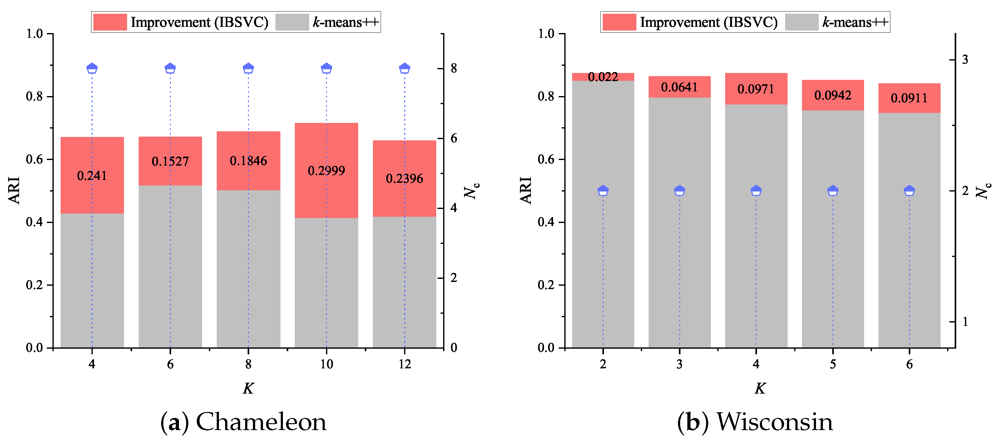
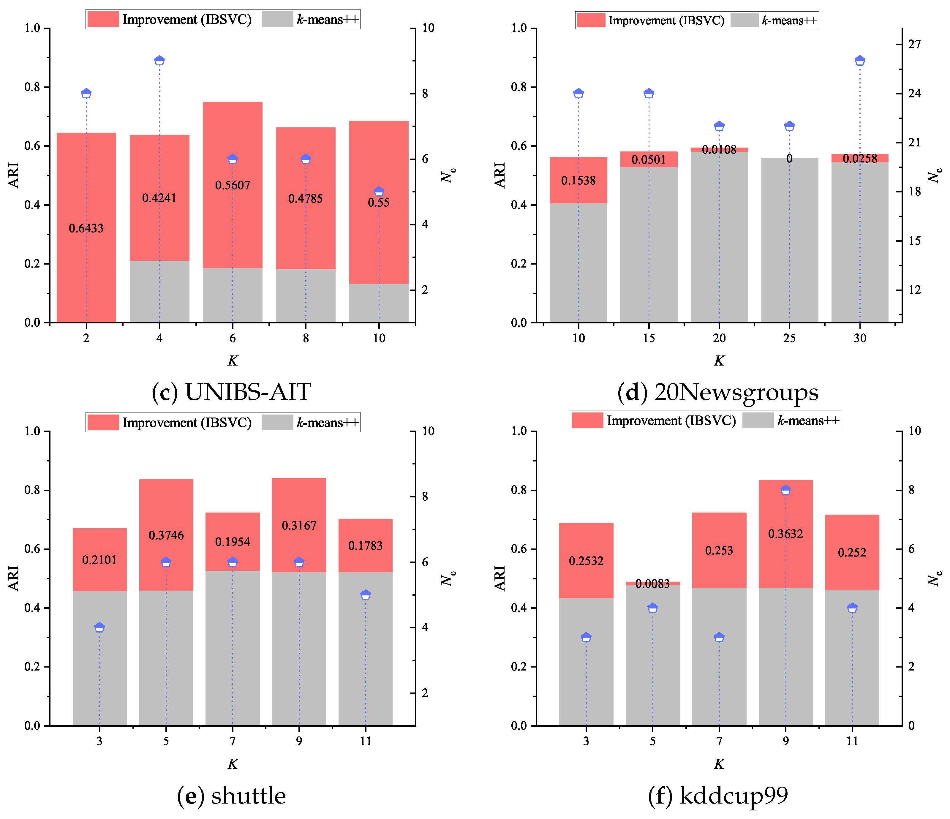
Without sufficient prior knowledge, the discovered cluster number $N_{\mathrm{c}}$ is a critical indicator that shows whether a method can capture data distribution accurately. Generally, if fake edge patterns cannot be eliminated appropriately, the discovered $N_{\mathrm{c}}$ is frequently greater than the ground truth. Meanwhile, if the noise data samples (or outliers) are not removed correctly, many more cluster prototypes (e.g., convex hulls in IBSVC) will be assumed to be connected, which reduces $N_{\mathrm{c}}$. Apparently, IBSVC, FRSVC, BSVC, and RSVC-EO often obtain an $N_{\mathrm{c}}$ decision, which is close or equivalent to the real number given in Table 2.

4.7. Finding Improvement Evidence over K-Means++

As shown in Figure 1, the k-means++ divides data into K subsets, which reduce the number of sample comparisons required by MBS. Although this leads to the appearance of fake edges, significant efficiency improvement is evident in Table 4. However, is k-means++ the major contributor to the accuracy? To answer this question, we conducted additional experiments for IBSVC to observe accuracy changes with respect to the baselines of the k-means++. Without the accurate prior knowledge K, we compared them with five different cluster numbers employed as the prior knowledge on these six datasets. The results are depicted in Figure 6, where the best accuracy in ten evaluations for each K is introduced. For each evaluation, IBSVC and k-means++ used the same K values.

In Figure 6, the horizontal axis represents the attempted K values. The left Y-axis corresponds to the achieved accuracies by the k-means++ (gray bar) and the corresponding improvements made by IBSVC (red bar). The numerical value marked on the red bar is the quantized improvement. As can be seen, there are significant improvements in accuracy, except for 20Newsgroup with $K=20,25$, Wisconsin with $K=2$, and $kddcup99$ with $K=5$. In fact, the corresponding K values are equivalent to or close to the ground truth of the class number (see Table 2). Since the k-means++ insists on dividing the data space into K clusters, we only present the number of clusters discovered by IBSVC using a scatter diagram, which refers to the right Y-axis. For most cases, the discovered cluster numbers $N_{\mathrm{c}}$ do not fluctuate dramatically with the change of K. In fact, $N_{\mathrm{c}}$ is also equivalent or close to the ground truth. As with the results above, IBSVC makes a major contribution to accuracy improvement. Meanwhile, clear evidence confirms the adaptive ability of IBSVC in cluster discovery. It performs stably even though there is no sufficient prior knowledge about K. Therefore, before setting K, the first thing we should consider is efficiency.

5. Related Works

Inspired by the support vector machine (SVM), SVC is well-known for its capability of handling arbitrary cluster shapes. However, evident challenges are also affecting its utilization, i.e., parameter selection, dual problem (2) solver, and cluster labeling. Recently, the latter two have received more attention, while few works have tried to tackle the first one, which is strongly related to the dual problem solver.

For the classic SVC, parameter selection includes the exploration of kernel width q, penalty factor C, and sample rate m. q is the major factor affecting the decomposition of clusters. For an optimal q, many works [1] limit it to $1/{max}_{i,j}\left|\right|{\mathbf{x}}_i-{\mathbf{x}}_j{\left|\right|}^2$ or $\frac{1}{2}({max}_{i,j}\left|\right|{\mathbf{x}}_i-{\mathbf{x}}_j{\left|\right|}^2-{min}_{i,j}\left|\right|{\mathbf{x}}_i-{\mathbf{x}}_j{\left|\right|}^2)$, and then incrementally increase it to force the cluster to split until an appropriate number of clusters is obtained. Another insightful work [34] defined a dissimilarity measure between basion cells (components of a cluster) by using a transition equilibrium vector (TEV); it then introduced a merging strategy to control the number of numbers. By restricting $R<1-\frac{1}{N}$, Lee and Daniels adopted a tangent approximation to yield an optimal q with fewer iterations. For these methods, the termination conditions can be either the available cluster number or the relatively stable region as the achieved cluster number changes. In fact, the former termination condition is difficult to determine without prior knowledge, similar to K for the k-means++. On the other hand, how to make the best choice from among the many stable regions is another challenge. Furthermore, before making the decision, many complete clustering processes that require pricey computation are inevitable.

In contrast, a consensus has been reached on the setting of C and m. Following [13], C is frequently set in order to control the number of BSVs or outliers, i.e., $n_{\mathrm{BSV}}<1/C$. Currently, along with the appearance of reconstructed dual problems [7,8], C is no longer considered important. The choice of the sample rate m is strongly related to the labeling strategy. Traditionally, it is set to any number from 10 to 20. By introducing a convex decomposition cluster labeling strategy [21], the average of m is reduced from 10 to 5 [7], and then to <2 [12]. Recently, [20] presented a novel connectivity analysis strategy for the labeling phase where sampling is no longer required.

A dual problem solver is the core of the training phase in which complex operations, huge iterations, and unaffordable memory by the pre-computed kernel matrix are critical and relevant tasks. To improve the robustness, [9] characterized the optimal sphere by introducing the first-order and second-order statistics. For complexity reduction, [4] rewrote the dual problem by introducing the Jaynes maximum entropy, while [35] started the solver with a position-based weight. Furthermore, [7] was the first work that directly utilized the relationship among the SVs to reformulate an equivalent model. Then, [8] transferred the traditional solvers to a dual coordinate descent (DCD) solver extended from [12]. The reconstruction process was also accompanied by the relaxation of constraints on the dual problem. Thus, the huge iterations were also effectively alleviated. For instance, statistical tests of [8,20] confirmed that the iteration number could be less than or equal to 10 with the DCD solver while obtaining acceptable results. It does not matter whether the original solver or the DCD solver is employed, the collected SVs for data description are a part of the whole data set. There, VCC [6] randomly selects $\theta N(\theta \in (0,1\left]\right)$ samples, while FSSVC [7] and BSVC [8] prefer the boundaries collected by BEPS [15] and its improved method SBS, respectively. In general, using cluster boundary to construct the objective dual problem can significantly reduce the memory consumption of the pre-computed kernel matrix from $O\left(N^2\right)$ to $O\left(N_{\mathrm{SV}}^2\right)$, where $N_{\mathrm{SV}}\ll N$. However, a small $N_{\mathrm{SV}}$ cannot have an efficient pattern description ability when dealing with high-dimensional data. Therefore, another feasible way is to calculate the kernel function on demand or to utilize a divide-and-conquer strategy [1]. However, bottlenecks frequently occur due to insufficient prior knowledge or self-adapted parameters, e.g., pricey time-consumption, instability, etc.

Cluster labeling is frequently related to the method types of the dual problem solver. For instance, various labeling strategies are widely accepted for the proposed IBSVC, similar to BSVC. The major consideration is whether strong dependence exists with the assumed cluster prototype. For the classic SVC, a complete graph (CG) leads to sampling between all the data sample pairs, while position-regularized SVC [35] reduces to SV-pairs. Inherited from a nonlinear dynamics system, R-CG [19] extracted SEVs as the cluster prototypes, whereas E-SVC [18,36] found the transition points (TS) for the connectivity analysis between the nearest neighboring basins. Both of them suffered from pricey iterations of seeking SEVs or TS. Another method using basin as the prototype appeared in [37], which introduced a cell growth strategy that starts at any data sphere, expands by absorbing new neighboring spheres, and splits if its density is reduced to a certain degree. Another strategy employs the convex hull as the prototype, which can be decomposed from any cluster. Sampling strategies for the connectivity analysis between two neighboring convex hulls can be linear [21], nonlinear [7], once sample [12], or no-sample [20,31]. CCL is a special strategy that checks the connectivity of two SVs through once distance calculation. However, overly strict constraints emphasized on the solver degrade its applicability. In fact, for these methods, the pricey consumption is the adjacent matrix, which usually ranges from $O\left(N_{\mathrm{SV}}^2\right)$ to $O\left(N^2\right)$.

Different from the aforementioned works, another insightful attempt [38] is the transfer of knowledge from the sphere of Equation (1) to the framework of k-means. Although k is still a requisite knowledge, it might serve as an inspiration to design ensemble learning with SVC.

6. Conclusions

For further performance improvements in boundary utilization and parameter selection, we proposed an IBSVC with self-adaption support for reasonable boundaries and comfortable parameters. As an improved method of BSVC, the first core idea was to reduce the comparisons in the whole data set, in which the vast majority of samples are useless for boundary determination. By introducing a divide-and-conquer strategy, MES was designed for edge pattern collection in local regions divided by the k-means++. Thus, the first series of self-adaption strategies were presented to remove the fake edges and retrain the outliers by adaptive data movement. Distinct from the state-of-the-art methods, the second core idea was to find the optimal kernel width q without prior knowledge that further contributes to the discovery of clusters. Accordingly, we proposed the second series of self-adaption strategies, which consist of a reasonable $\beta$ initialization method for the improvement of the effectiveness of iteration control in the proposed iSolver, and an FPS method that automatically determines the kernel width q by simple computations. FPS tries to reduce the difference between the data description drawn by the possibly formed model and the actual pattern that does not require any result from tentative cluster analyses. Due to the absence of restrictions on prototype types, IBSVC contributes to the first phase of cluster analysis and accepts various labeling strategies. For simplicity, we chose a convex decomposition-based strategy in order to complete cluster checking and labeling. Experimental results confirm that IBSVC greatly restrains the unstable influence of the k-means++ while achieving excellent efficiency and applicability.

Although IBSVC features efficiency and parameter self-adaptation, further improvements in the accuracy and flexibility of the matrix construction in iSolver have become ever-lasting issues. How to make the setting of the step size in MES and the determination of the kernel width q more elaborate and intelligent are worthy of further investigations.

References

- Li, H.; Ping, Y. Recent Advances in Support Vector Clustering: Theory and Applications. Int. J. Pattern Recogn. Artif. Intell. 2015, 29, 1550002. [Google Scholar] [CrossRef]
- Jin, T.; Gao, X. Overcoming The Error of Optical Power Measurement Caused by The Curvature Radius. Opt. Express 2022, 30, 17115–17129. [Google Scholar] [CrossRef]
- Arslan, G.; Madran, U.; Soyoğlu, D. An Algebraic Approach to Clustering and Classification with Support Vector Machines. Mathematics 2022, 10, 128. [Google Scholar] [CrossRef]
- Guo, C.; Li, F. An Improved Algorithm for Support Vector Clustering based on Maximum Entropy Principle and Kernel Matrix. Expert Syst. Appl. 2011, 38, 8138–8143. [Google Scholar] [CrossRef]
- Jung, K.H.; Lee, D.; Lee, J. Fast support-based clustering method for large-scale problems. Pattern Recogn. 2010, 43, 1975–1983. [Google Scholar] [CrossRef]
- Kim, K.; Son, Y.; Lee, J. Voronoi Cell-Based Clustering Using a Kernel Support. IEEE Trans. Knowl. Data Eng. 2015, 27, 1146–1156. [Google Scholar] [CrossRef]
- Ping, Y.; Chang, Y.; Zhou, Y.; Tian, Y.; Yang, Y.; Zhang, Z. Fast and Scalable Support Vector Clustering for Large-scale Data Analysis. Knowl. Inf. Syst. 2015, 43, 281–310. [Google Scholar] [CrossRef]
- Ping, Y.; Hao, B.; Li, H.; Lai, Y.; Guo, C.; Ma, H.; Wang, B.; Hei, X. Efficient Training Support Vector Clustering with Appropriate Boundary Information. IEEE Access 2019, 7, 146964–146978. [Google Scholar] [CrossRef]
- Wang, Y.; Chen, J.; Xie, X.; Yang, S.; Pang, W.; Huang, L.; Zhang, S.; Zhao, S. Minimum Distribution Support Vector Clustering. Entropy 2021, 23, 1473. [Google Scholar] [CrossRef]
- Li, C.; Wang, N.; Li, W.; Li, Y.; Zhang, J. Regrouping and Echelon Utilization of Retired Lithium-ion Batteries based on A Novel Support Vector Clustering Approach. IEEE Trans. Transp. Electrif. 2022, 1–11. [Google Scholar] [CrossRef]
- Lee, S.H. Gaussian Kernel width Selection and Fast Cluster Labeling for Support Vector Clustering. Ph.D. Thesis, University of Massachusetts Lowell, Lowell, MA, USA, 2005. [Google Scholar]
- Ping, Y.; Tian, Y.; Guo, C.; Wang, B.; Yang, Y. FRSVC: Towards Making Support Vector Clustering Consume Less. Pattern Recogn. 2017, 69, 286–298. [Google Scholar] [CrossRef]
- Ben-Hur, A.; Horn, D.; Siegelmann, H.T.; Vapnik, V.N. Support Vector Clustering. J. Mach. Learn. Res. 2001, 2, 125–137. [Google Scholar] [CrossRef]
- Ting, K.M.; Wells, J.R.; Zhu, Y. Point-Set Kernel Clustering. IEEE Trans. Knowl. Data Eng. 2022, 41–51. [Google Scholar] [CrossRef]
- Li, Y.H.; Maguire, L. Selecting Critical Patterns Based on Local Geometrical and Statistical Information. IEEE Trans. Pattern Anal. Mach. Intell. 2011, 33, 1189–1201. [Google Scholar]
- Karypis, G.; Han, E.H.; Kumar, V. Chameleon: A Hierarchical Clustering Algorithm Using Dynamic Modeling. Computer 1999, 32, 68–75. [Google Scholar] [CrossRef]
- Ping, Y.; Zhou, Y.; Yang, Y. A Novel Scheme for Accelerating Support Vector Clustering. Comput. Inform. 2012, 31, 1001–1026. [Google Scholar]
- Lee, J.; Lee, D. Dynamic Characterization of Cluster Structures for Robust and Inductive Support Vector Clustering. IEEE Trans. Pattern Anal. Mach. Intell. 2006, 28, 1869–1874. [Google Scholar] [PubMed]
- Lee, J.; Lee, D. An Improved Cluster Labeling Method for Support Vector Clustering. IEEE Trans. Pattern Anal. Mach. Intell. 2005, 27, 461–464. [Google Scholar]
- Ping, Y.; Hao, B.; Hei, X.; Wu, J.; Wang, B. Maximized Privacy-Preserving Outsourcing on Support Vector Clustering. Electronics 2020, 9, 178. [Google Scholar] [CrossRef]
- Ping, Y.; Tian, Y.; Zhou, Y.; Yang, Y. Convex Decomposition Based Cluster Labeling Method for Support Vector Clustering. J. Comput. Sci. Technol. 2012, 27, 428–442. [Google Scholar] [CrossRef]
- Arthur, D.; Vassilvitskii, S. k-means++: The Advantages of Careful Seeding. In Proceedings of the Eighteenth Annual ACM-SIAM Symposium on Discrete Algorithms (SODA ’07), New Orleans, LA, USA, 7–9 January 2007; pp. 1027–1035. [Google Scholar]
- Frank, A.; Asuncion, A. UCI Machine Learning Repository. 2010. Available online: http://archive.ics.uci.edu/ml (accessed on 1 June 2022).
- Lang, K. NewsWeeder: Learning to filter netnews. In Proceedings of the 12th International Conference on Machine Learning, (ICML’95), Tahoe City, CA, USA, 9–12 July 1995; pp. 331–339. [Google Scholar]
- Ping, Y.; Zhou, Y.; Xue, C.; Yang, Y. Efficient representation of text with multiple perspectives. J. China Univ. Posts Telecommun. 2012, 19, 101–111. [Google Scholar] [CrossRef]
- UNIBS. The UNIBS Anonymized 2009 Internet Traces. 18 March 2010. Available online: http://www.ing.unibs.it/ntw/tools/traces (accessed on 1 June 2022).
- Peng, J.; Zhou, Y.; Wang, C.; Yang, Y.; Ping, Y. Early TCP Traffic Classification. J. Appl. Sci. Electron. Inf. Eng. 2011, 29, 73–77. [Google Scholar]
- Guo, C.; Zhou, Y.; Ping, Y.; Zhang, Z.; Liu, G.; Yang, Y. A Distance Sum-based Hybrid Method for Intrusion Detection. Appl. Intell. 2014, 40, 178–188. [Google Scholar] [CrossRef]
- UCI Lab. KDD Cup 1999 Intrusion Detection Dataset. 28 October 1999. Available online: http://kdd.ics.uci.edu/databases/kddcup99/kddcup99.html (accessed on 1 June 2022).
- Xu, R.; Wunsch, D.C. Clustering. In Clustering; John Wiley & Sons: Hoboken, NJ, USA, 2008. [Google Scholar]
- Lee, S.H.; Daniels, K.M. Cone Cluster Labeling for Support Vector Clustering. In Proceedings of the 6th SIAM International Conference on Data Mining, Bethesda, MD, USA, 20–22 April 2006; pp. 484–488. [Google Scholar]
- Rathore, P.; Ghafoori, Z.; Bezdek, J.C.; Palaniswami, M.; Leckie, C. Approximating Dunn’s Cluster Validity Indices for Partitions of Big Data. IEEE Trans. Cybern. 2019, 49, 1629–1641. [Google Scholar] [CrossRef]
- Garcia, S.; Herrera, F. An Extension on “Statistical Comparisons of Classifiers over Multiple Data Sets” for all Pairwise Comparisons. J. Mach. Learn. Res. 2008, 9, 2677–2694. [Google Scholar]
- Lee, D.; Lee, J. Dynamic Dissimilarity Measure for Support-based Clustering. IEEE Trans. Knowl. Data Eng. 2010, 22, 900–905. [Google Scholar] [CrossRef]
- Wang, C.D.; Lai, J.H. Position Regularized Support Vector Domain Description. Pattern Recogn. 2013, 46, 875–884. [Google Scholar] [CrossRef]
- Lee, D.; Jung, K.H.; Lee, J. Constructing Sparse Kernel Machines Using Attractors. IEEE Trans. Pattern Anal. Mach. Intell. 2009, 20, 721–729. [Google Scholar]
- Chiang, J.H.; Hao, P.Y. A New Kernel-based Fuzzy Clustering Approach: Support Vector Clustering with Cell Growing. IEEE Trans. Fuzzy Syst. 2003, 11, 518–527. [Google Scholar] [CrossRef]
- Gonitz, N.; Lima, L.A.; Muller, K.R.; Kloft, M.; Nakajima, S. Support Vector Data Descriptions and k-Means Clustering: One Class? IEEE Trans. Neural Netw. Learn. Syst. 2018, 29, 3994–4006. [Google Scholar] [CrossRef]