Introducing the ReaLISED Dataset for Sound Event Classification

Abstract

This paper presents the Real-Life Indoor Sound Event Dataset (ReaLISED), a new database which has been developed to contribute to the scientific advance by providing a large amount of real labeled indoor audio event recordings. They offer the scientific community the possibility of testing Sound Event Classification (SEC) algorithms. The full set is made up of 2479 sound clips of 18 different events, which were recorded following a precise recording process described along the proposal. This, together with a described way of testing the similarity of new audio, makes the dataset scalable and opens up the door to its future growth, if desired by the researchers. The full set presents a good balance in terms of the number of recordings of each type of event, which is a desirable characteristic of any dataset. Conversely, the main limitation of the provided data is that all the audio is recorded in indoor environments, which was the aim behind this development. To test the quality of the dataset, both the intraclass and the interclass similarities were evaluated. The first has been studied through the calculation of the intraclass Pearson correlation coefficient and further discard of redundant audio, while the second one has been evaluated with the creation, training and testing of different classifiers: linear and quadratic discriminants, k-Nearest Neighbors (kNN), Support Vector Machines (SVM), Multilayer Perceptron (MLP), and Deep Neural Networks (DNN). Firstly, experiments were carried out over the entire dataset, and later over three different groups (impulsive sounds, non-impulsive sounds, and appliances) composed of six classes according to the results from the entire dataset. This clustering shows the usefulness of following a two-step classification process.

1. Introduction

Nowadays, there is a growing interest in smart environments (e.g., smart cities, smart buildings, smart homes), which are spaces where a set of sensors, actuators and many other computational elements provide services for betterment of human life [1]. In these places, a large number of applications can be developed by combining advanced sensory systems based on cameras, microphones, motion sensors, etc., and communication and signal processing systems. Application examples include fields such as identification and discrimination of microseismic events [2,3], or pavement monitoring and analysis [4]. These types of systems aim to improve the quality of life of humans in several aspects such as security, safety, and comfort, among others. Acoustic sensors are potentially important in these smart environments, since applying the proper sound processing techniques to the sound waves we can extract information about the sound sources, their positions, and about the environment in which sensing is carried out. Furthermore, these sensors can work with or without light, they are inexpensive, and the computational requirements for implementing algorithms are affordable, given that the required sampling rates are relatively low.

Sound processing in smart environments seeks in many cases to solve the problem of Sound Event Classification (SEC), which consists in recognizing the set of active sounds in a given audio signal. An example of a growing field where acoustic recognition is applied is speech emotion recognition [5,6,7]. Classification is performed once a sound event is detected, task that is solved by a Sound Event Detection (SED) algorithm, which detects the onset and offset of sounds in a given audio signal [8]. These approaches have a key role in different applications, such as the design of “Health Smart Homes” which provide health care services for people with special needs who wish to remain independent and to live in their own home [9], the security systems in public transport [10], and the field of surveillance systems in general [11].

One of the most relevant challenges in both SEC and SED fields is the Detection and Classification of Acoustic Scenes and Events (DCASE). The current challenge (DCASE 2022) [12], is divided into six different tasks, such as “Low-complexity Acoustic Scene Classification”, which aims to classify acoustic scenes (urban park, metro station, public square, etc.). The second task, called “Unsupervised Anomalous Sound Detection for Machine Condition Monitoring Applying Domain Generalization Techniques”, consists in identifying whether the sound emitted by a target machine is normal or anomalous. Another task strongly associated to the present work is carried out in “Sound Event Detection in Domestic Environments” (task 4), where new systems are developed for SED using real data, which are unlabeled, weakly labeled or strongly labeled with time stamps.

SEC has been approached using several machine learning methods, such as Hidden Markov Models [13] and Gaussian Mixture Models [14]. Other approaches use more recent methods, as in [15,16,17], where Convolutional Recurrent Neural Network and Support Vector Machines (SVM) are applied, respectively. Recently, other approaches have used Deep Neural Networks (DNN) [18], but a large dataset is necessary.

In all cases the use of an appropriate dataset of sounds is crucial. Several examples of recent acoustic datasets for SEC, which consist of several audio clips and the labels explaining the class presented in each clip, can be found in the literature. As far as we know, the largest one at the moment is AudioSet, proposed in [19], which consists of more than 1.7 million audio clips of more than 500 classes from different acoustic scenes, with multiple event labels per clip. Its main advantage is the well-structured hierarchy (6 levels), which covers a great amount of different sounds of each class. All clips were taken from YouTube videos, without taking the real environment into account. Due to the huge size of this dataset, the use of big data techniques would be feasible, as more amount of data enables the use of more deeper and complex learning methods [20]. However, this database does not provide the waveform but audio features which makes the research on SEC more difficult, as new features cannot be calculated. To overcome some problems of AudioSet, the FDS50K set is proposed in [21], an open set based on sounds from the online platform FreeSound, using a hierarchy similar to the AudioSet one. This set is composed of 51 k audio clips of 200 weakly labeled classes of everyday sounds, which are not recorded in real scenarios. In [22], the set GISE-51 is proposed, which is composed of 1.6 k sound clips of 51 isolated sound events which belong to event types such as vehicles, environmental, musical instrument, speech, and others. These sounds are also mixed with other soundscapes to complete the set. Another audio set called TUT is presented in [14], with sounds recorded in streets, parks and homes, covering 15 different acoustic environments. In the case of TUT-Home, the set is composed of different human-labeled clips grouped into 11 classes of an average of 60 audio samples of 30 s length. These general sets are based on audio sounds taken from another greater set, which generally are extracted from platforms such as YouTube or FreeSound, so the main issue is that new recordings are not provided. Another drawback is the fact that the background sound is not recorded with the audio event, but is artificially added. In addition, they are not oriented to the domestic environment, with the exception of the last one, the TUT-Home set. Other proposals oriented their sets to urban sounds, such as SONYC, presented in [23] and used in DCASE 2019. This set is made up of 3 k real sounds recorded in New York, representing 23 sound events grouped into eight different human labeled classes. Other proposals are aimed at other types of environments and applications, such as detecting the malfunction of industrial machines [24,25].

The dataset presented in [26] is composed of three different kinds of sound sources (material, noise, and music) recorded in an anechoic chamber. The real scenario was simulated by the convolution of these sounds and an impulse response, considering a linear and stable transmission channel. The authors collected some impulse responses in different locations, using a variable reverberating room, and considering reverberation times between 0.01 and 2 s. The problem with this methodology is the lack of real audios, being all of them simulated. Another case is presented in [16], where information about coordinates is enclosed for the location.

Another public dataset oriented to domestic sounds is DESED, presented in [27] and used in DCASE challenge for SED. It is composed of 10 domestic sound classes taken from AudioSet and others synthetically generated. CHiME-Home [28] uses seven human-labeled classes of domestic sounds and consists of 4378 clips of 4 s recorded by a binaural recorder and labeled by three people. Its main drawback is that the recordings only take place in one house, so it could not provide sounds generalized to other spaces. In addition, some of the classes seem to be too general, such as percussive sounds or broadband noise, while others are too specific, such as adult male, adult female or child speech. Another dataset [29] is composed of 11 event classes recorded at several realistic positions in two different rooms, resulting in a total of 5 h of duration. However, the recordings of this dataset focus on SED for office environments, so its purpose and proposed classes are not directly applicable to the domestic sphere.

Developing a new acoustic dataset has its advantages and disadvantages. On the one hand, it allows having a wide variety of new labeled events recorded by several people in real environments. This is important because real recordings include the room impulsive response instead of adding synthetically the room reverberation afterwards. On the other hand, this development involves a big investment of time and resources for recording, trimming and labelling each audio individually.

This paper proposes a new audio dataset called ReaLISED, composed of 18 different classes and 2479 clips recorded in real scenarios. The proposed dataset is very diverse in the places where the sounds were recorded and in the kinds of audio sources (windows, doors, objects, etc.). The ultimate objective of this proposal is to provide a real, heterogeneous and rich dataset susceptible to be used in several studies, and thus contribute to solve some important issues present in nowadays societies. The dataset is focused on domestic sounds but it is scalable to other sounds and scenarios. It includes the real waveforms of isolated sounds that also can be used to propose and calculate new features useful for SED or SEC, or to apply deep-learning based detectors or classifiers fed directly with the sound waveform instead of pre-calculated features.

The paper is divided into the following sections. First, Section 2 shows a detailed description of the proposed database. Later, in Section 3 and Section 4 both the intraclass and interclass similarities are studied. After that, the experiments and results carried out are presented in Section 5. Finally, Section 6 shows the conclusions drawn from the presented proposal.

2. Description of the Database

The ReaLISED (Real-Life Indoor Sound Event Dataset) is a new database recorded, labeled and developed by the authors of the present proposal. It is composed of eighteen (18) different events. Some of them are related to daily household tasks, such as cooking, walking or cleaning, and others include sounds produced by humans or other objects present in a house. The event classes are the following: beater, cooking, cupboard/wardrobe, dishwasher, door, drawer, furniture movement, microwave, object falling, smoke extractor, speech, switch, television, vacuum cleaner, walking, washing machine, water tap, and window. There are 2479 clips of isolated sounds, which result in 3624.51 s (slightly more than one hour).

Apart from the labels related to the class of event, extra information for each recording is provided in order to be exploited if necessary in the future, with other research purposes. This extra information completes the description of the sound source. For example, in events related to objects such as doors, windows, wardrobes or drawers, the action taken during the clip is specified, e.g., opening or closing. Another example of extra information is the material in which an object has fallen when the class is “object falling”. In addition, descriptions of events such as furniture movement, door, window, cupboard, and vacuuming are accompanied by labels with information about the material they are made of.

The recordings were made in different locations, including apartments, semi-detached houses, and the Polytechnic School of University of Alcalá. The reason for choosing this heterogeneous set of environments is to try to generalise as much as possible the impulse responses of the rooms. This would allow the development of classifiers that, working with real signals, focus on the event class information rather than on the environment in which the sound source is located.

Four Olympus LS-100 recorders [30] were used during the recording process. They are equipped with a high-performance directional stereo microphone and a quality amplifier circuit, with a characteristic frequency response with a lower cut-off frequency of 20 Hz and an upper cut-off frequency of 20 kHz, and with an upper sound pressure limit of 140 dBSPL. The coding format can be chosen between the linear PCM with a sampling rate of 96.0/88.2/48.0/44.1 kHz and 16/24 bits per sample, and MP3 with 320/256/128/64 kbps bitrate.

The recording process of the dataset was based on a robust protocol that included rules about the parameters selected on the recorder and its proximity to the source. The sampling frequency was set to 44.1 kHz and 24 bits per sample, which is enough to sample signals with 20 kHz bandwidth and dynamic range up to 144 dB. The stereo mode was used although one channel was discarded later, and a medium sensitivity of the microphone was set, which corresponds to 94 dBSPL, to avoid saturation of sounds, even though it was checked that saturation did not take place in the recorder sound before starting the records. Regardless, the audio was later revised and those which still presented saturation were discarded. Apart from that, the distance between the recorder and the sound source was set to approximately 30–40 cm.

In

Table 1. Summary of the dataset characteristics, including the number of audios, the average duration and the impulsivity or non-impulsivity of the different classes.

Event Class	Number of Audios	Average Duration (s)	Impulsive Sound (Yes/No)
Beater	126	1.02	No
Cooking	176	1.01	No
Cupboard/Wardrobe	156	0.96	Yes
Dishwasher	130	1.01	No
Door	109	1.75	Yes
Drawer	158	1.34	Yes
Furniture movement	152	1.18	No
Microwave	124	1.03	No
Object falling	119	0.49	Yes
Smoke extractor	142	1.01	No
Speech	190	4.03	No
Switch	108	0.24	Yes
Television	143	2.18	No
Vacuum cleaner	166	1.26	No
Walking	119	2.67	No
Washing machine	117	1.01	No
Water tap	140	1.40	No
Window	104	1.74	Yes

, the description of the dataset is summarized. It includes the event class recorded in each audio, the number of recordings (audios) of each class, the average duration of each class (in seconds), and the impulsivity or not impulsivity of the class. The impulsivity of this audio is characterized by a short duration, an abrupt onset, and a rapid decay [31]. The number of events in each class is between 104 for the “Window” class and 190 for the “Speech” class, with a mean value of 138 events and a standard deviation of 25. The average duration depends on the type of sound, with the shortest in the impulsive sound classes (“Object falling”, “Switch”), and the longest for the classes where the sound source is a person (“Speech”, “Walking”).

The dataset is introduced to the scientific community by providing all the .flac files which composed it. The name of the files is built with 5 pieces of information, separated with underscores (“_”), with the format “$abc\_123\_45\_67\_8.flac$”. In the following lines the meaning of each part of the name is explained:

• “abc”: the first three letters indicate the source that produces the sound. This segment can take 18 different values: ‘bea’ (beater), ‘coo’ (cooking), ‘cup’ (cupboard/wardrobe), ‘dis’ (dishwasher), ‘doo’ (door), ‘dra’ (drawer), ‘fur’ (furniture movement), ‘mic’ (microwave), ‘obj’ (object falling), ‘smo’ (smoke extractor), ‘spe’ (speech), ‘swi’ (switch), ‘tel’ (television), ‘vac’ (vacuum cleaner), ‘wal’ (walking), ‘was’ (washing machine), ‘wat’ (water tap), ‘win’ (window).
• “123”: this set of digits identifies the event among the number of events produced by the source identified with “abc”. This segment can take all the values between ‘001’ and ‘190’, which is the maximum number of events of a particular class we can find in the dataset (speech).
• “45”: this set of digits identifies the action that produces the sound. This segment can take 11 different values: ‘01’ (close), ‘02’ (open), ‘03’ (throw), ‘04’ (turn on), ‘05’ (turn off), ‘06’ (move), ‘07’ (plug), ‘08’ (unplug), ‘09’ (raise), ‘10’ (lower), and ‘00’ (there is no information about the action).
• “67”: this set of digits identifies the material the sound source is made of. This segment can take 14 different values: ’01’ (wood), ’02’ (glass), ’03’ (metal), ’04’ (plastic), ’05’ (ceramic), ’06’ (synthetic), ’07’ (cardboard), ’08’ (marble), ’09’ (floating platform), ’10’ (platelet), ’11’ (wicker), ’12’ (carpet), ’13’ (medium-density fibreboard MDF), and ’00’ (there is no information about the material).
• “8”: the last digit gives approximate information about the intensity of the recorded sound. It can take 4 different values: ’1’ (low intensity), ’2’ (medium intensity), ’3’ (high intensity), ’0’ (there is no information about the intensity).

For clarity, some examples of audio file names with this code are shown hereunder:

• “doo_040_02_00_3.flac” is the name of the 40th file in the “door” class, described as “opening a door of unknown material with high intensity”.
• “fur_058_06_01_2.flac” is the name of the 58th file in the “furniture movement” class, described as “moving a wooden furniture with medium intensity”.
• “vac_001_00_00_0.flac” is the name of the 1st audio file in the “vacuum cleaner” class, described as “using the vacuum cleaner, without information about the action, neither the material or the intensity”.

The full dataset is available and can be downloaded from [32].

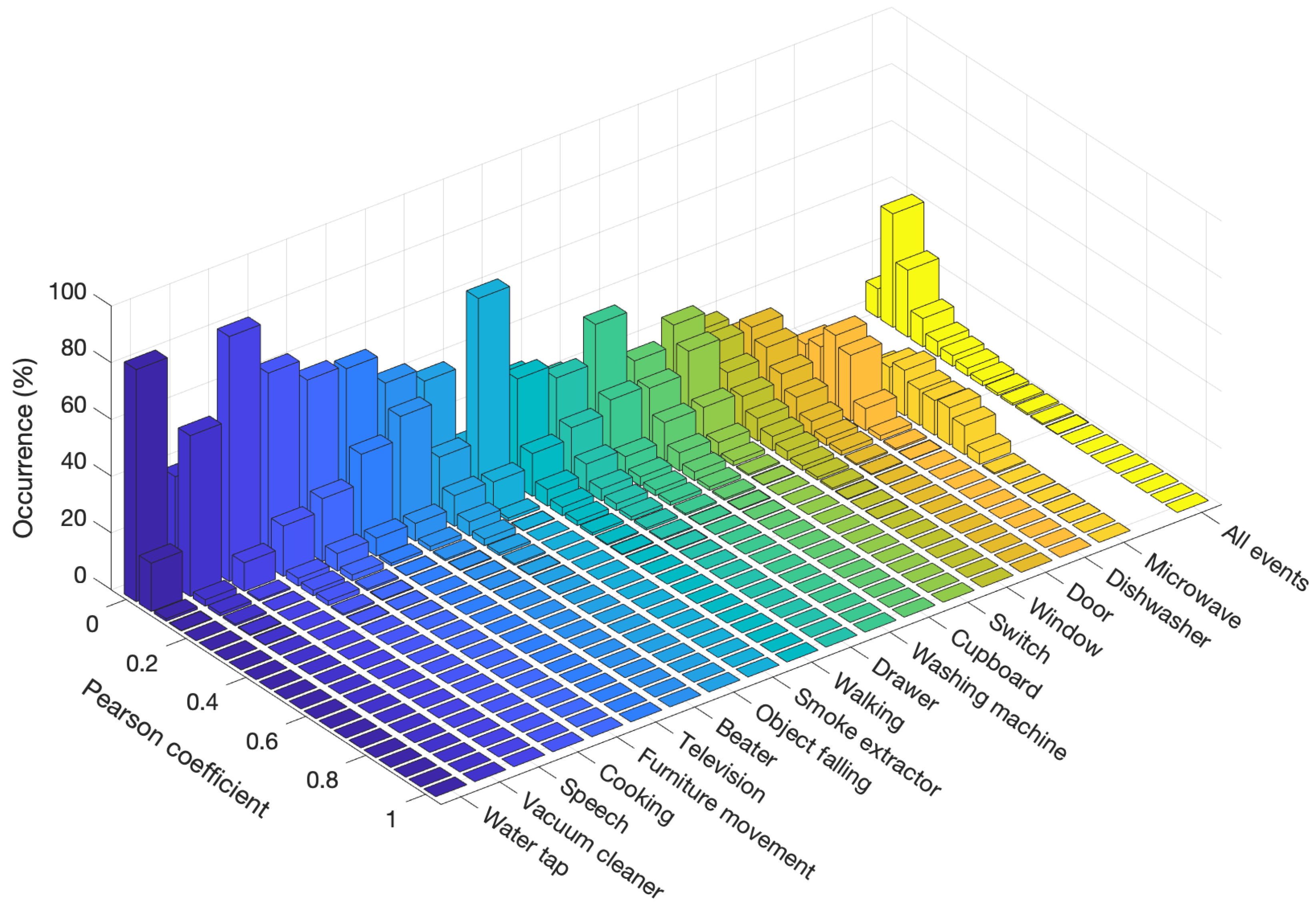
3. Intraclass Similarity

One of the key issues in any new database proposal is how to ensure and measure its quality. The quality assessment must ensure that data are consistent, there are neither duplicated data nor duplicated identifiers, and there are no missing values, or incomplete or imprecise metadata [33]. In this sense, all data, metadata and identifiers were reviewed following a standard procedure.

Furthermore, we measured the intraclass Pearson correlation coefficient, to find sound events with similar information. Events that are similar should be detected with the objective of keeping only one of them, since the rest would not provide relevant new information and would be unbalancing the database. The maximum Pearson correlation coefficient r of two different discrete signals $x_1\left[n\right]$ and $x_2\left[n\right]$, is determined by evaluating the maximum of the cross correlation of the signals, divided by the standard deviation of each of the two signals [34], as shown in Equation (1). It is important to highlight that the average value of each signal must be removed previously to the evaluation of the cross-correlation.

$$r=\frac{\underset{m}{max}\left(E_n\left\{(x_1\left[n\right]-{\overline{x}}_1)(x_2[n-m]-{\overline{x}}_2)\right\}\right)}{\sqrt{E_n\left\{{(x_1\left[n\right]-{\overline{x}}_1)}^2\right\}{E}_n\left\{{(x_2\left[n\right]-{\overline{x}}_2)}^2\right\}}},$$

(1)

where m is the shift applied to the signal $x_2\left[n\right]$, ${\overline{x}}_i=E_n\left\{x_i\left[n\right]\right\}$ represent the average value of the signal $x_i$, and $E\{·\}$ represent the expected value.

This r parameter gives us an idea of the similarity between the signals. If in any case this value is very close to unity, one of the two signals should be discarded from the database. So, to measure the similarity of the database, we measured the cross-correlation over the signals belonging to a given class. It is important to highlight that the comparison must be made between signals of the same class.

4. Interclass Similarity

When using a database for SEC, it is not only necessary to ensure that sound events within a class are loosely correlated, but it is also necessary to know the similarity between classes that could affect the performance of the classifiers. For this purpose, a set of classifiers was created, trained and tested, and the results obtained have allowed us to know which classes are most similar to each other and which give rise to the highest number of classification errors.

The general scheme of the classification process is presented in Figure 1. In the first stage, every audio signal is divided into frames of 20 ms and the features are extracted to obtain valuable information for the following stage. Once the relevant information is obtained, the classifier assigns each audio signal to one of the classes. To guarantee the validity of results, k-fold cross-validation method is used. Furthermore, several metrics are used in order to be compared easily for future works. These parts are defined in this section as follows.

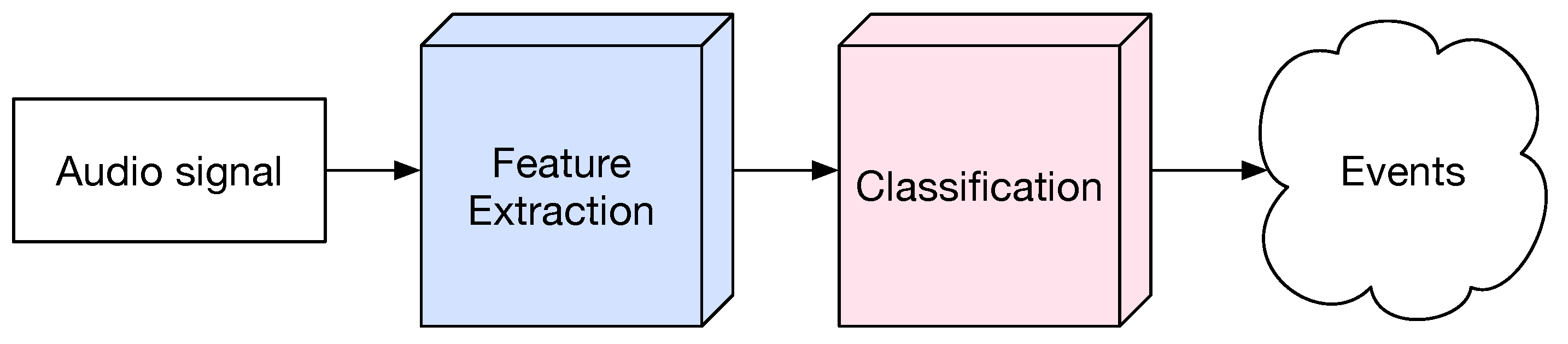
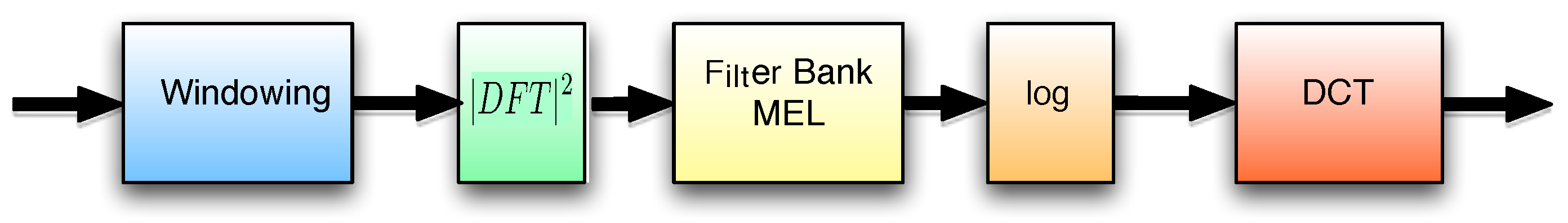
4.1. Feature Extraction

The feature extraction stage determines the relevant information for classification from each audio signal. In this work, features are obtained by calculating MFCCs (Mel-Frequency Cepstral Coefficients) and some statistical parameters. MFCCs have been regarded as one of the essential techniques of parametrization used in audio and speech processing [35]. Perceptual analysis pretends to emulate the human ear non-linear frequency response by creating a set of filters on non-linearly spaced frequency bands. Mel cepstral analysis uses the Mel scale and a cepstral smoothing to get the final smoothed spectrum. The procedure can be found in [36] and is presented in the scheme shown in Figure 2.

This scheme is composed of five blocks or tasks. The first task is windowing, in which the signal is divided into several short-time overlapping segments to avoid loss of information. Each segment is windowed and the squared magnitude of the Discrete Fourier Transform (DFT) is obtained. The next block is the filter bank, in which the frequency domain information of the previous block is multiplied by a set of triangular shape frequency response filters whose bandwidth is directly related to the central frequency in the band. The output of this block is a vector which elements are the summation of the weighted frequency components in each band. The next block applies a logarithmic function to the previous result, and this is the input to the last block, where the Discrete Cosine Transform (DCT) is applied. The spectral coefficients are transformed to the frequency domain, that is, they are converted into cepstral coefficients.

Once MFCCs are obtained, features are calculated as some statistics of the MFCCs set. Some of the most commonly used statistics are the mean and the standard deviation. It is also normal to use statistics from differential values of the MFCCs, denominated delta MFCC or ΔMFCCs. These ΔMFCCs are determined using Equation (2).

$$\Delta MFC{C}_{ft}=MFC{C}_{ft}-MFC{C}_{f(t-d)},$$

(2)

being f-th the triangular filter of the t-time frame and d the differentiation shift. The features used by the classifiers are the mean of the MFCCs, the standard deviation of the MFCCs, and the standard deviation of the $\Delta MFCCs$ with $d=2$. Related to the number of MFCCs, 5, 15 and 20 coefficients were tested to study the impact of this parameter on the SEC task. Therefore, there will be a total of 4 feature sets: the one which calculates 5 MFCCs (15 features in total), the one which calculates 15 MFCCs (45 features in total), the one which computes 20 MFCCs (60 features in total), and the one which combines the previous three sets (120 features in total).

4.2. Classification Stage

The classification stage assigns the input pattern to one of the classes, being the pattern the input vector composed of the extracted features. The classifiers used in this work are the following:

• Least Squares Linear Classifier (LSLC), where the values of the weights of the linear combinations are those that minimize the Mean Squared Error (MSE) obtaining the Wiener-Hopf equations [37].
• Least Squares Quadratic Classifier (LSQC). This classifier linearly combines first and second degree combinations of the input data, generally obtaining better results than the LSLC without greatly increasing the computational complexity [38].
• k-Nearest Neighbors (kNN). This classifier measures the distance of the input vector x to k vectors representing the class in question and choosing the class with the smallest average distance [39].
• Support Vector Machine (SVM) with linear kernel [40]. SVMs project the observation vector to a higher dimensional space, using a set of kernel functions. The centers of the kernel functions are chosen from the design set and are denominated “support vectors”. Once the observation vector is projected, a linear discriminant is used to determine the SVM’s output and take the decision.
• Multilayer Perceptron (MLP). It consists of three layers of nodes (one input layer, one hidden layer and one output layer). Except for the input nodes, each node is a neuron that uses a nonlinear activation function. The most common type of neuron is McCulloch–Pitts neuron [41], which consists of a weighted sum of the inputs, followed by the application of a non-linear function (sigmoidal function or hyperbolic tangent, commonly). In this work, MLPs were trained with the Scaled Conjugate Gradient training function, a fast supervised learning algorithm [42].
• Deep Neural Networks (DNN). It consists of at least four layers of nodes (one input layer, two or more hidden layers and one output layer). This type of classifier is an extension of the MLP included within deep learning techniques.

4.3. Validation Stage

To test the results adequately, cross-validation methods were used to reduce overfitting (generalization loss) and maximize the accuracy in estimating the classification error rate. Specifically, we used the k-fold cross-validation consisting in partitioning the dataset into k different folds and running k times the whole design process. So, for each experiment, a given fold is used as the test set, and the remaining $k-1$ folds are used as the design set. The absolute error is averaged over the k experiments. In the present case, the data were divided into $k=4$ folds. It must be noted that the events are proportionally distributed in each of them before the sound processing take place. This ensure an adequate balance in the experiments so that it is avoided the emergence of low prediction accuracies when some algorithms try to classify rare categories in a dataset. The dataset was divided into a set used for training and a set used for testing, being the 75% of the events assigned to the training set and the 25% to the test set. Additionally, this process is repeated 10 times to minimize the randomization of the experiments. Finally, the results considered and presented later are the average of the results of each experiment.

4.4. Evaluation Metrics

To evaluate the obtained results, we used several parameters. These are the Accuracy (ACC), Precision (P), Recall (R), and F1-Score (F1):

• ACC is calculated using the number of True Positives (TP), True Negatives (TN), False Positives (FP) and False Negatives (FN):

  $$ACC(\%)=\frac{TP+TN}{TP+TN+FP+FN}·100$$

  (3)
• P and R are defined as follows:

  $$P(\%)=\frac{TP}{TP+FP}·100$$

  (4)

  $$R(\%)=\frac{TP}{TP+FN}·100$$

  (5)
• Once we have the values of P and R, F1 is directly calculated as shown in Equation (6).

  $$F1(\%)=\frac{2·P·R}{P+R}·100$$

  (6)

5. Experiments and Results

This section shows the experiments carried out and the obtained results to show the properties of the dataset. The results of the analysis of intraclass similarity were used to discard similar sound events. Only those events whose information is not similar to that of other events of the same type in the database are kept. The resulting database was applied to the interclass similarity analysis, mainly based on the analysis of classification results.

5.1. Results of Intraclass Similarity Analysis

Figure 3 shows the distribution of the maximum values of the Pearson correlation coefficients (r), which were computed according to Equation (1), when comparing all the possible pairs of different events within the same class. Each column of the figure (displayed in a different color) represents the histogram of the r values that were obtained for a given class in the database, so the taller the height of the column bar the more frequent that range of r value is obtained. The average histogram taking into account all the events is also displayed in yellow in the rightmost part of the figure. From the results, none of the pairs have a Pearson correlation coefficient greater than 0.9. Furthermore, 99% of the comparisons between instances gave r values lower than 0.8, and 95% of the comparisons were concentrated between 0 and 0.6. All this indicates the level of consistency of the files in the database, as the similarity between audio from the same class is very small according to the Pearson correlation coefficient (r).

The sound event classes with worse similarity results are “Microwave” and “Dishwasher”, as their r values are mainly concentrated in the 0.2–0.4 range. They are two examples of household appliances which produce stationary sounds that tend to present larger r values. To increase the number of uncorrelated sound events, very different models of these appliances might be used. This task will be completed in a future work.

The sound events maintained in the database present a low correlation between them, which is indicative that they share little information, concluding that the database was generated so that the ratio between the amount of information and the number of events is high. This is a desirable property to properly train a classification system, as the richness and diversity of data always contributes to making more generalized and robust algorithms.

5.2. Results of Interclass Similarity Analysis

Different classifiers were trained and tested, to infer if the classes are linearly separable or not, and if they could be separated in the features domain or is better to project the features to a higher dimension space where the classes are linearly separable. In addition, knowledge of the similarity measure between the classes included in the database is interesting to explore the possibility of using layered classification strategies. The number of features is another parameter tested. In the case of MLP, where one hidden layer is used, the number of neurons tested has taken values in powers of two: 8 neurons (MLP8), 16 neurons (MLP16), …, 512 neurons (MLP512). In the case of DNN, different numbers of neurons and different number of hidden layers were tested: 2 (DNN2), 3 (DNN3), …, 5 (DNN5). For reasons of simplification, only the most significant results will be presented. In the case of using DNN, all the experiments presented have hidden layers made up of 128 neurons.

5.2.1. Interclass Analysis with the Whole Set of Classes

First of all, we trained and tested classifiers to classify the whole set of sound event classes, to find out the classes of events with the highest probability of confusion. The results were used to define the groups or categories of sound events with similar characteristics that are responsible for most of the confusions.

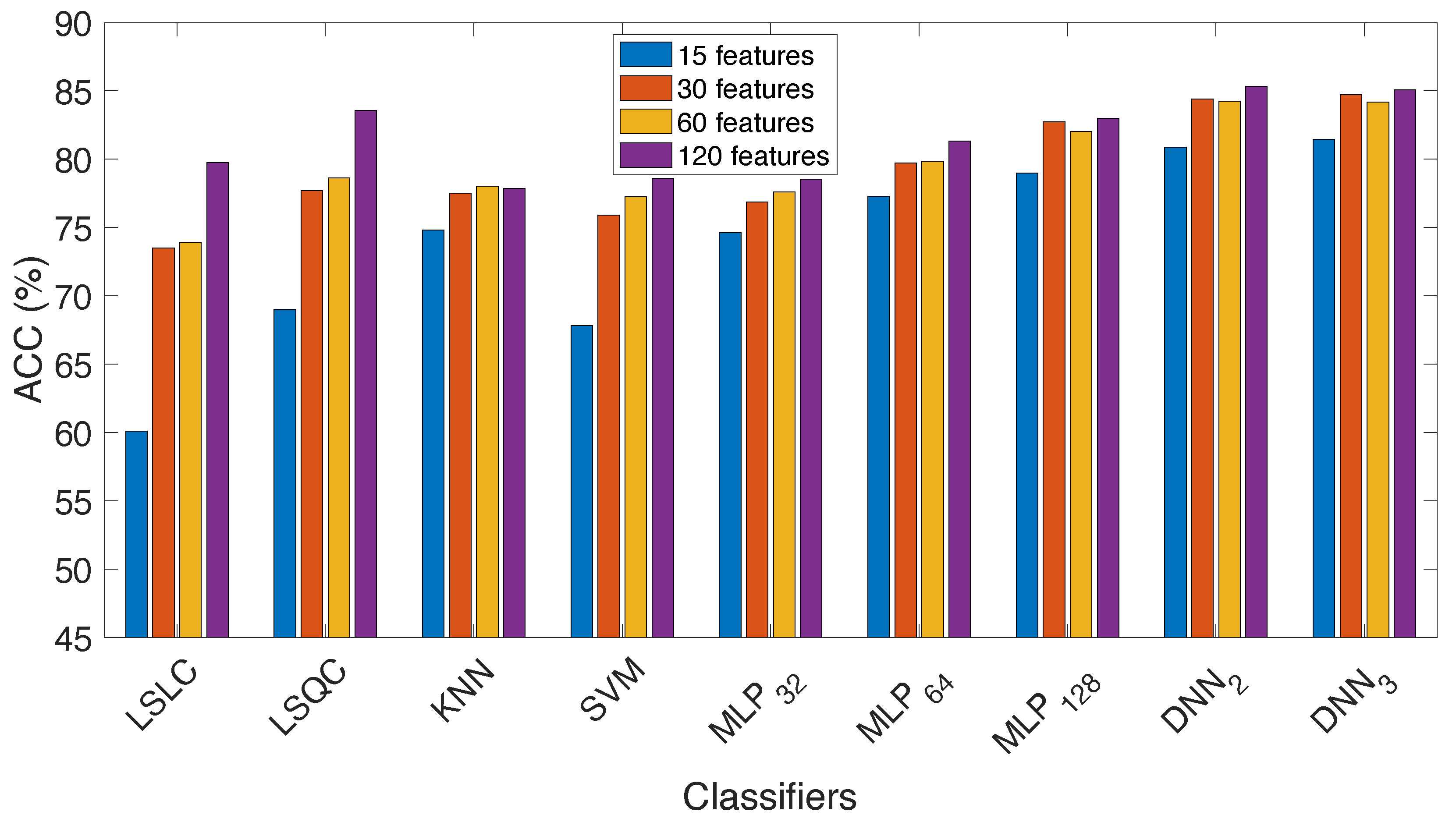
• In Figure 4, the ACC is represented according to the classifiers used and the number of features selected. It is observed that the more features used, the better results are obtained for all classifiers. The best results are obtained when combining the three sets of MFCCs (120 features). When the sets are tested separately, the number of MFCCs that gets the best results is 20 in most cases (60 features), followed closely by 15 MFCCs (45 features). The classifiers most sensitive to the number of features are LSLC, LSQC and SVM, while the performance of the rest of them is not as dependent on the number of features. Regarding the classifiers applied, the best results are obtained when using the DNN with two hidden layers (DNN2) and the LSQC.

Figure 4. ACC values obtained when applying the seven classifiers mentioned in Section 4.2, and selecting different number of features.

Figure 4. ACC values obtained when applying the seven classifiers mentioned in Section 4.2, and selecting different number of features.

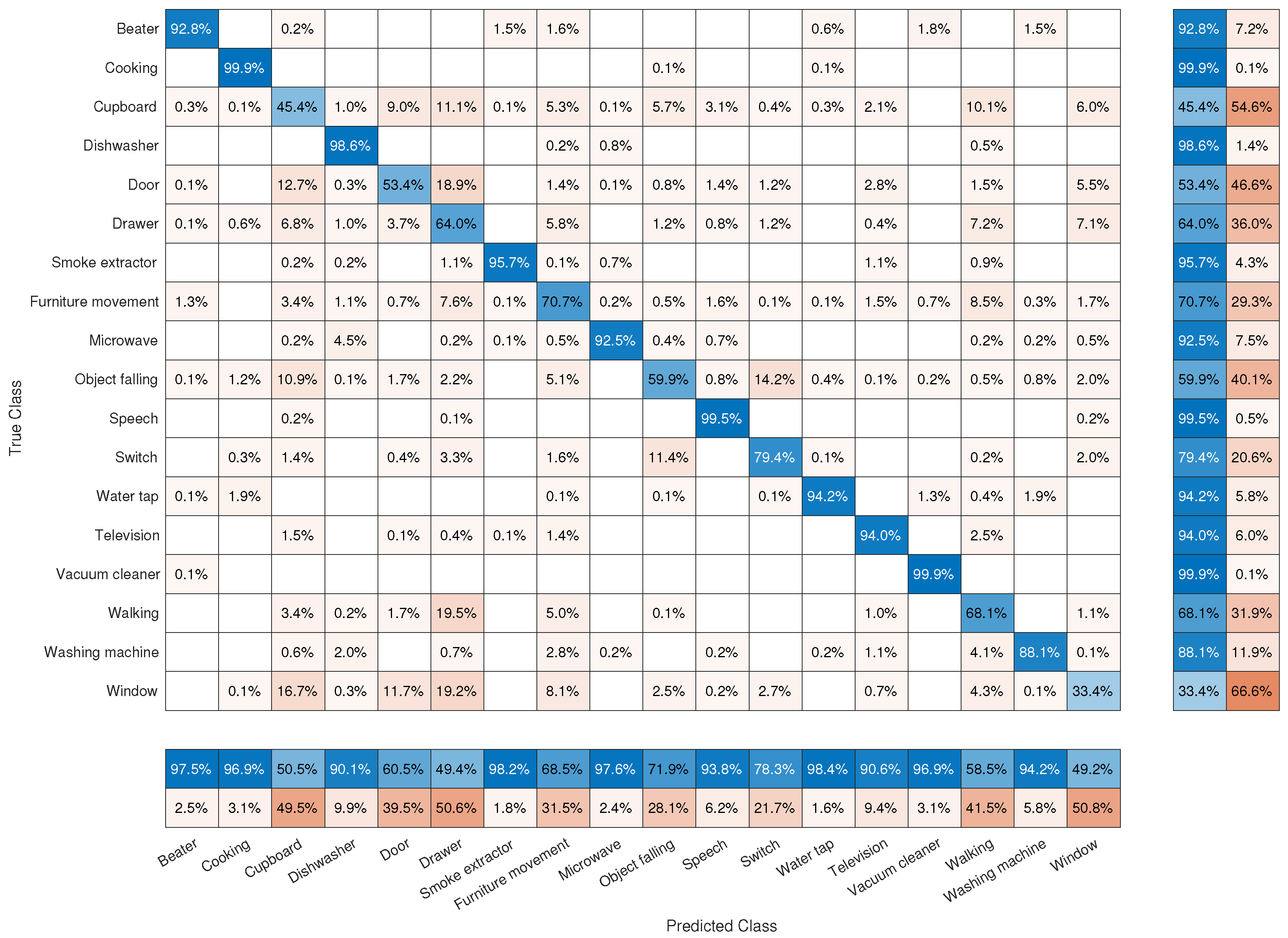
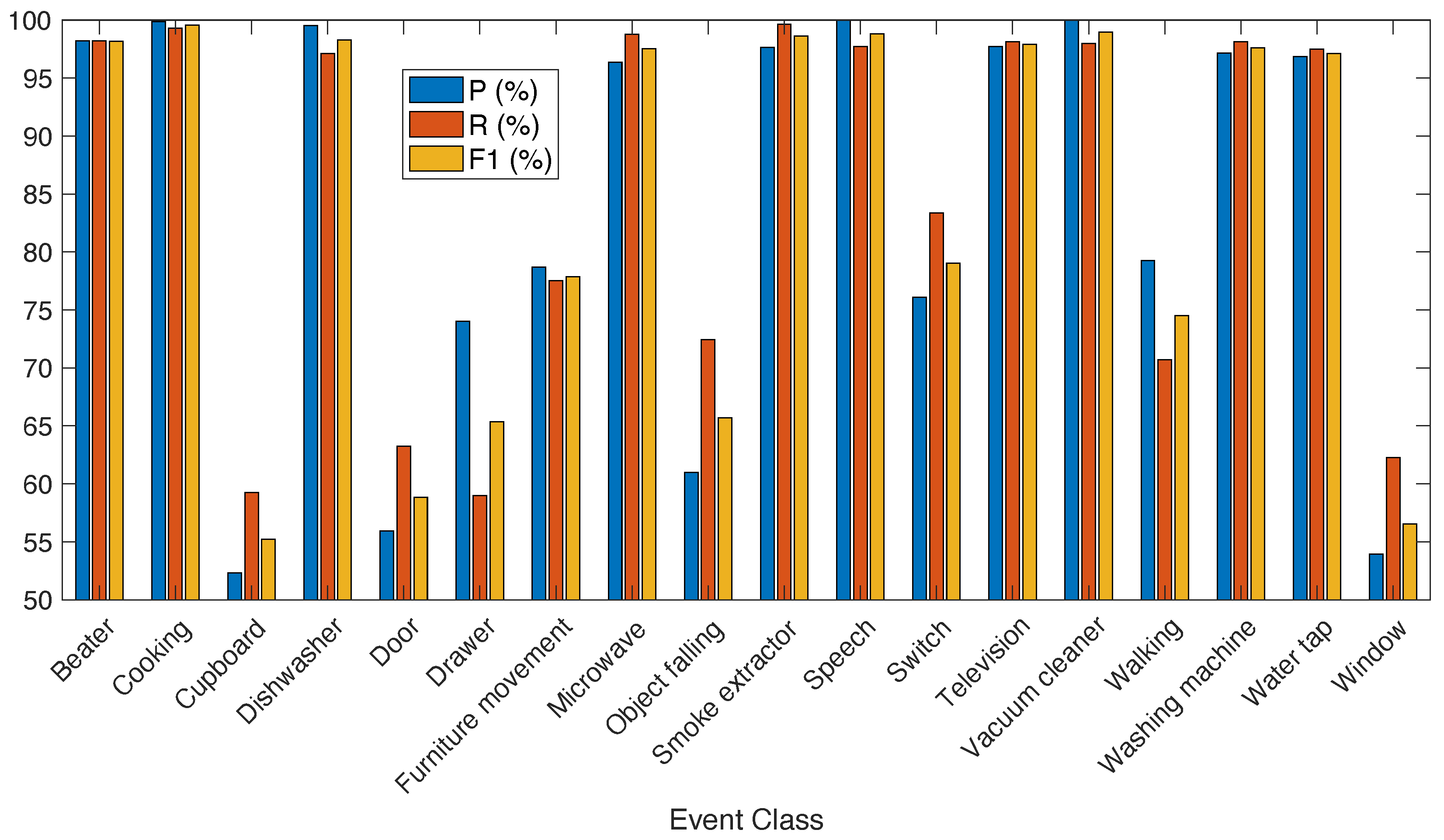
• The results of ACC, P, R and F1, obtained with the whole set of event classes using the complete set of features (120) are presented in Table 2. The best results are obtained using the DNN2, getting 85.33% of ACC and 84.44% of F1. If we focus on machine learning based classifiers, the best results are provided by the LSQC, which gets 83.58% of ACC and 82.12% of F1. These results also indicate that the problem of SEC with this database can only be solved satisfactorily if the number of free parameters in the classifier is high. Therefore, the performance with simpler classifiers such as LSLC, kNN or SVM are worse.

Table 2. Results obtained when testing the full dataset with the maximum number of features (120).

Classifier	ACC (%)	P (%)	R (%)	F1 (%)
LSLC	79.75	78.25	78.59	77.69
LSQC	83.58	82.24	82.82	82.12
kNN	77.86	76.45	77.40	76.53
SVM	78.62	77.54	76.72	76.55
MLP32	78.55	76.67	77.96	76.55
MLP64	81.34	79.65	80.88	79.79
MLP128	83.01	81.53	82.86	81.74
DNN2	85.33	84.15	85.02	84.44
DNN3	85.09	83.86	84.73	84.17

Table 2. Results obtained when testing the full dataset with the maximum number of features (120).

Classifier	ACC (%)	P (%)	R (%)	F1 (%)
LSLC	79.75	78.25	78.59	77.69
LSQC	83.58	82.24	82.82	82.12
kNN	77.86	76.45	77.40	76.53
SVM	78.62	77.54	76.72	76.55
MLP32	78.55	76.67	77.96	76.55
MLP64	81.34	79.65	80.88	79.79
MLP128	83.01	81.53	82.86	81.74
DNN2	85.33	84.15	85.02	84.44
DNN3	85.09	83.86	84.73	84.17

The confusion matrix obtained when testing all the events with the DNN2 using 120 features is shown in Figure 5. It must be noted that these results include the average of the 4-fold cross-validation method and the 10 repetitions of the experiment. The vertical axis represents the true classes (labels) and the horizontal axis represents the assigned classes (outputs of classifiers). A summary of the results from the columns and rows can be shown at the right and the bottom of the figure. It can be observed that most events are classified very well (more than 90% of the tested events of these classes are correctly classified). These classes are “beater”, “cooking”, “dishwasher”, “smoke extractor”, “microwave”, “speech”, “water tap”, “television”, and “vacuum cleaner”.

The worst classified classes are “window”, “cupboard” and “door”, since only 33.4% of windows, 45.4% of cupboards and 53.4% of doors sound events are correctly assigned to the corresponding class. These classes are confused mainly with “drawers”, and with each other. The class “furniture movement” is easily confused with “walking” class, although it does not happen the same in the contrary. In fact, “walking” is usually confused with “drawer”. Besides, “object falling” gives rise to many errors in classification, since it is easily confused with many other classes, especially “switch” and “cupboard”.

In order to analyze the classification results within each event class, we present the results in terms of ACC, P, R, and F1 in Figure 6. The results presented are those obtained with the DNN2 (2 hidden layers). Regarding the event classes, some of them (beater, cooking, dishwasher, microwave, smoke extractor, speech, television, vacuum cleaner, washing machine and water tap) are classified very well, reaching more than 95% of F1. They correspond to non-impulsive events or events produced by different appliances. On the contrary, the worst results are obtained with impulsive sounds (produced by cupboards, doors, drawers, object falling, switches and windows). This suggests to carry out a previous classification into impulsive and non-impulsive events to improve the classification results. Furthermore, some event classes are more prone to be misclassified due to FP errors (cupboard, door, object falling, switch, window), as their P is substantially smaller than their R. For its part, in drawer and walking classes the errors are mainly produced by the large number of FN.

5.2.2. Interclass Analysis by Grouping the Classes

The events were grouped according to the types of sounds to know the performance of classifiers when the sound events have similar acoustic properties, making classification more difficult. Three different groups were proposed, composed of six classes each, according to the results in the previous subsection.

• Group 1: Impulsive sound events, is composed of six different classes: cupboard/wardrobe, door, drawer, object falling, switch, and window. In

  Table 3. Event classes that make up Group 1: Impulsive sound events, as well as the number of audios and length of each of them.

  Event Class	Number of Files	Length (s)
  Cupboard/Wardrobe	156	149.52
  Door	109	119.89
  Drawer	158	121.47
  Object falling	119	38.43
  Switch	108	26.03
  Window	104	181.21

  , the event class, the number of files and their lengths are shown.

• Group 2: Non-impulsive sound events encompasses six different events: furniture movement, speech, television, vacuum cleaner, walking, and water tap.

  Table 4. Event classes that make up Group 2: Non-impulsive sound events, as well as the number of audios and length of each of them.

  Event Class	Number of Files	Length (s)
  Furniture movement	152	178.78
  Speech	190	764.86
  Television	143	311.87
  Vacuum cleaner	166	208.58
  Walking	119	317.52
  Water tap	140	196.25

  shows the classes, the number of files in each class, and their lengths.

• Group 3: Appliances includes six classes of sound events produced typically in the kitchen by different household appliances and by a person which is cooking (e.g., frying, roasting): beater, cooking, dishwasher, microwave, smoker extractor, and washing machine.

  Table 5. Event classes that make up Group 3: Appliances, as well as the number of audios and length of each of them.

  Event Class	Number of Files	Length (s)
  Beater	126	128.67
  Cooking	176	177.85
  Dishwasher	130	131.72
  Microwave	124	125.64
  Smoke extractor	142	144.10
  Washing Machine	117	117.88

  shows the classes, the number of files in each class, and their lengths.

Hereinafter, the results were obtained with the maximum number of features selected (120). The following tables show the ACC, P, R, and F1 in percentage for each group of events using the different classifiers. It must be noted that the F1 was calculated by averaging the F1 values obtained with the different events groups, folds (as k-fold cross-validation is applied) and number of repetitions of the experiment, so the value obtained when replacing the values of P and R from the table to the F1 equation will not correspond to the F1 value showed. It applies to all the tables showed in this section.

Firstly,

Table 6. Results obtained when testing Group 1: Impulsive sound events with different classifiers.

Classifier	ACC (%)	P (%)	R (%)	F1 (%)
LSLC	76.48	75.38	75.41	75.26
LSQC	75.94	75.22	75.02	75.03
kNN	73.44	72.43	72.50	72.32
SVM	73.22	70.96	71.36	70.51
MLP32	76.54	75.12	75.49	75.17
MLP64	76.25	74.96	74.88	74.78
MLP128	76.74	75.59	75.77	75.56
DNN2	76.26	75.02	75.32	74.97
DNN3	77.21	76.07	76.30	76.09

shows the aforementioned parameters in the case of testing Group 1 (impulsive events). The best performance is obtained with the DNN3 in terms of ACC (77.21%) and F1 (76.09%), followed closely by the LSLC. In general, the complexity of the classifiers does not substantially affect the performance in Group 1. Regarding the values of P and R, they are very similar to each other for all the classifiers. This means the misclassified events are due to FP and FN in equal proportion.

The results obtained for the next combination of events, Group 2 (non-impulsive events), are showed in

Table 7. Results obtained when testing Group 2: Non-impulsive sound events with different classifiers.

Classifier	ACC(%)	P (%)	R (%)	F1 (%)
LSLC	75.08	74.66	75.61	75.04
LSQC	77.48	76.93	77.39	77.11
kNN	76.63	76.15	76.79	76.35
SVM	73.20	72.98	74.34	73.47
MLP32	76.91	76.40	78.11	77.08
MLP64	76.64	76.19	77.86	76.82
MLP128	76.78	76.28	77.43	76.76
DNN2	77.67	77.19	78.83	77.82
DNN3	77.75	77.38	79.11	78.03

. In this case, the best results of ACC and F1 are obtained with the DNN3 (77.75% and 78.03%, respectively), but the LSQC from the traditional machine learning methods also gets proper results (77.48% of ACC and 77.11% of F1). In this case, it can be observed that R is better than P for all the classifiers. It means that the errors made by the system are due to the number of FP rather than to the number of FN.

Table 8. Results obtained when testing Group 3: Appliances with different classifiers.

Classifier	ACC (%)	P (%)	R (%)	F1 (%)
LSLC	83.29	82.17	82.40	82.21
LSQC	83.66	82.65	82.92	82.60
kNN	79.44	78.02	78.58	77.93
SVM	80.83	79.31	79.56	79.36
MLP32	83.55	82.52	82.86	82.53
MLP64	83.64	82.53	82.78	82.58
MLP128	83.80	82.77	83.17	82.74
DNN2	83.64	82.57	83.00	82.63
DNN3	84.34	83.36	83.67	83.36

shows the results obtained when testing Group 3 (appliances). In this case, the best results are obtained with the DNN3, achieving 84.34% of ACC and 83.36% of F1, although other classifiers such as LSLC, LSQC or and MLP present really close values. With Group 3, the results are better than with the previous ones (between 6 and 8 points of ACC, depending on the classifier applied). This may be due to the distinctive sound of the different appliances, which can make them easily separable.

These results show a high similarity among the classes included in each group, but a low similarity between two classes of different groups, so it may be interesting to approach the problem of classifying sound events in two stages. In a first one, we would classify between groups of events, and in a second one, we would classify between classes within each group. This strategy will be probably developed in a future work.

6. Conclusions

In this proposal, a dataset composed of real indoor audio is presented for SEC tasks. The characteristics of the different events, the recording conditions and the experiments were explained. The dataset is composed of 2479 sound events, belonging to 18 sound classes. The number of sound events in each class ranges from 104 to 190, with a mean value of 138 events per class and a standard deviation of 25 events. The sampling frequency is 44.1 kHz and each sample is encoded in PCM with 24 bits. The large number of sound event classes gives the database sufficient generality to be used in a wide range of applications.

The sound events included in each class were carefully chosen to maximize the amount of information for the size of the database. To achieve this, a sound event is included in the dataset if the correlation with other sound events in the same class is low, thus minimizing redundancy.

The sound database includes classes of sound events with similar properties, in order to be used to train and test classifiers in very demanding applications with similar sound sources. The sound event classes can be grouped into three large groups, with six similar classes each. Within each group, the classes have a certain similarity, but the classes of different groups are not similar. This is evident because it is easy to correctly classify sounds belonging to classes of different groups, but it is more complicated to correctly classify sounds of classes included in the same group. Additionally, we tried to ensure that the sound events included in the same class are poorly correlated with each other, thus increasing the ratio between the amount of information and the number of events.

This clustering allows the database to be used to train simple classifiers or complex classifiers, and also to address the problem of classifying the 18 sound classes in two stages. The first stage would consist of a simple classifier to distinguish between groups and the second stage would consist of a more complex classifier to distinguish between similar classes.

Finally, it should be noted that this database is scalable. As the conditions of the sound recording are described in detail, more events could be easily added, as long as the properties of bandwidth and number of bits per sample are maintained. In addition, a procedure for deciding whether or not a sound event is added to the database, based on the correlation with sounds of the same class, was proposed and should be followed in the future when increasing the number of sound events in the database, so as to avoid including sounds that add little new information. The main limitation of the provided dataset is that all the audio is recorded in indoor environments, which was the aim behind this development.

References

1. Ambika, N. Secure and Reliable Knowledge-Based Intrusion Detection Using Mobile Base Stations in Smart Environments. In Encyclopedia of Information Science and Technology, 4th ed.; IGI Global: Hershey, PA, USA, 2021; pp. 500–513. [Google Scholar]
2. Dong, L.J.; Tang, Z.; Li, X.B.; Chen, Y.C.; Xue, J.C. Discrimination of mining microseismic events and blasts using convolutional neural networks and original waveform. J. Cent. South Univ. 2020, 27, 3078–3089. [Google Scholar] [CrossRef]
3. Peng, K.; Tang, Z.; Dong, L.; Sun, D. Machine Learning Based Identification of Microseismic Signals Using Characteristic Parameters. Sensors 2021, 21, 6967. [Google Scholar] [CrossRef]
4. Hou, Y.; Li, Q.; Zhang, C.; Lu, G.; Ye, Z.; Chen, Y.; Wang, L.; Cao, D. The state-of-the-art review on applications of intrusive sensing, image processing techniques, and machine learning methods in pavement monitoring and analysis. Engineering 2021, 7, 845–856. [Google Scholar] [CrossRef]
5. Kwon, S. Att-Net: Enhanced emotion recognition system using lightweight self-attention module. Appl. Soft Comput. 2021, 102, 107101. [Google Scholar]
6. Kwon, S. MLT-DNet: Speech emotion recognition using 1D dilated CNN based on multi-learning trick approach. Expert Syst. Appl. 2021, 167, 114177. [Google Scholar]
7. Zhu-Zhou, F.; Gil-Pita, R.; García-Gómez, J.; Rosa-Zurera, M. Robust Multi-Scenario Speech-Based Emotion Recognition System. Sensors 2022, 22, 2343. [Google Scholar] [CrossRef]
8. Adavanne, S.; Fayek, H.; Tourbabin, V. Sound event classification and detection with weakly labeled data. In Proceedings of the Detection and Classification of Acoustic Scenes and Events 2019 Workshop (DCASE2019), New York, NY, USA, 25–26 October 2019. [Google Scholar]
9. Vacher, M.; Portet, F.; Fleury, A.; Noury, N. Development of audio sensing technology for ambient assisted living: Applications and challenges. Int. J. E-Health Med. Commun. 2011, 2, 35–54. [Google Scholar] [CrossRef]
10. Rouas, J.L.; Louradour, J.; Ambellouis, S. Audio events detection in public transport vehicle. In Proceedings of the 2006 IEEE Intelligent Transportation Systems Conference, Toronto, ON, Canada, 17–20 September 2006; pp. 733–738. [Google Scholar]
11. Clavel, C.; Ehrette, T.; Richard, G. Events detection for an audio-based surveillance system. In Proceedings of the 2005 IEEE International Conference on Multimedia and Expo, Amsterdam, The Netherlands, 6 July 2005; pp. 1306–1309. [Google Scholar]
12. DCASE2022 Challenge. Challenge on Detection and Classification of Acoustic Scenes and Events. Available online: https://dcase.community/challenge2022/ (accessed on 27 May 2022).
13. Diment, A. Sound event detection for office live and office synthetic AASP challenge. In Proceedings of the IEEE AASP Challenge on Detection and Classification of Acoustic Scenes and Events, New Paltz, NY, USA, 20–23 October 2013. [Google Scholar]
14. Mesaros, A.; Heittola, T.; Virtanen, T. TUT database for acoustic scene classification and sound event detection. In Proceedings of the 2016 24th European Signal Processing Conference (EUSIPCO), Budapest, Hungary, 29 August–2 September 2016; pp. 1128–1132. [Google Scholar] [CrossRef]
15. Adavanne, S.; Pertilä, P.; Virtanen, T. Sound event detection using spatial features and convolutional recurrent neural network. In Proceedings of the 2017 IEEE International Conference on Acoustics, Speech and Signal Processing (ICASSP), New Orleans, LA, USA, 5–9 March 2017; pp. 771–775. [Google Scholar]
16. Adavanne, S.; Politis, A.; Virtanen, T. A multi-room reverberant dataset for sound event localization and detection. arXiv 2019, arXiv:1905.08546. [Google Scholar]
17. Foggia, P.; Petkov, N.; Saggese, A.; Strisciuglio, N.; Vento, M. Reliable detection of audio events in highly noisy environments. Pattern Recognit. Lett. 2015, 65, 22–28. [Google Scholar] [CrossRef]
18. Ciaburro, G.; Iannace, G. Improving Smart Cities Safety Using Sound Events Detection Based on Deep Neural Network Algorithm. Informatics 2020, 7, 23. [Google Scholar] [CrossRef]
19. Gemmeke, J.F.; Ellis, D.P.W.; Freedman, D.; Jansen, A.; Lawrence, W.; Moore, R.C.; Plakal, M.; Ritter, M. Audio Set: An ontology and human-labeled dataset for audio events. In Proceedings of the 2017 IEEE International Conference on Acoustics, Speech and Signal Processing (ICASSP), New Orleans, LA, USA, 5–9 March 2017; pp. 776–780. [Google Scholar] [CrossRef]
20. Yiu, C. The big data opportunity. Policy Exch. 2012, 1, 36. [Google Scholar]
21. Fonseca, E.; Favory, X.; Pons, J.; Font, F.; Serra, X. FSD50K: An Open Dataset of Human-Labeled Sound Events. arXiv 2020, arXiv:2010.00475. [Google Scholar] [CrossRef]
22. Yadav, S.; Foster, M.E. GISE-51: A scalable isolated sound events dataset. arXiv 2021, arXiv:2103.12306. [Google Scholar]
23. Cartwright, M.; Mendez, A.E.M.; Cramer, J.; Lostanlen, V.; Dove, G.; Wu, H.H.; Salamon, J.; Nov, O.; Bello, J. SONYC Urban Sound Tagging (SONYC-UST): A multilabel dataset from an urban acoustic sensor network. In Proceedings of the Detection and Classification of Acoustic Scenes and Events 2019 Workshop (DCASE2019), New York, NY, USA, 25–26 October 2019. [Google Scholar]
24. Purohit, H.; Tanabe, R.; Ichige, K.; Endo, T.; Nikaido, Y.; Suefusa, K.; Kawaguchi, Y. MIMII Dataset: Sound Dataset for Malfunctioning Industrial Machine Investigation and Inspection. arXiv 2019, arXiv:1909.09347. [Google Scholar]
25. Koizumi, Y.; Saito, S.; Uematsu, H.; Harada, N.; Imoto, K. ToyADMOS: A Dataset of Miniature-Machine Operating Sounds for Anomalous Sound Detection. In Proceedings of the 2019 IEEE Workshop on Applications of Signal Processing to Audio and Acoustics (WASPAA), New Paltz, NY, USA, 20–23 October 2019; pp. 313–317. [Google Scholar] [CrossRef] [Green Version]
26. Nakamura, S.; Hiyane, K.; Asano, F.; Nishiura, T.; Yamada, T. Acoustical sound database in real environments for sound scene understanding and hands-free speech recognition. In Proceedings of the 2nd International Conference on Language Resources and Evaluation, Athens, Greece, 31 May–2 June 2000. [Google Scholar]
27. Turpault, N.; Wisdom, S.; Erdogan, H.; Hershey, J.; Serizel, R.; Fonseca, E.; Seetharaman, P.; Salamon, J. Improving Sound Event Detection In Domestic Environments Using Sound Separation. arXiv 2020, arXiv:2007.03932. [Google Scholar]
28. Foster, P.; Sigtia, S.; Krstulovic, S.; Barker, J.; Plumbley, M.D. Chime-home: A dataset for sound source recognition in a domestic environment. In Proceedings of the 2015 IEEE Workshop on Applications of Signal Processing to Audio and Acoustics (WASPAA), New Paltz, NY, USA, 18–21 October 2015; pp. 1–5. [Google Scholar]
29. Brousmiche, M.; Rouat, J.; Dupont, S. SECL-UMons Database for Sound Event Classification and Localization. In Proceedings of the ICASSP 2020–2020 IEEE International Conference on Acoustics, Speech and Signal Processing (ICASSP), Barcelona, Spain, 4–8 May 2020; pp. 756–760. [Google Scholar]
30. Olympus. Multi-Track Linear PCM Recorder LS-100 User’s Manual; Olympus: Tokyo, Japan, 2012. [Google Scholar]
31. Pedersen, T. Audibility of impulsive sounds in environmental noise. In Proceedings of the 29th International Congress on Noise Control Engineering, Nice, France, 27–28 August 2000; pp. 4158–4164. [Google Scholar]
32. Mohino-Herranz, I.; Garcia-Gomez, J.; Aguilar-Ortega, M.; Utrilla-Manso, M.; Gil-Pita, R.; Rosa-Zurera, M. Real-Life Indoor Sound Event Dataset (ReaLISED) for Sound Event Classification (SEC). Available online: https://zenodo.org/record/6488321 (accessed on 5 June 2022).
33. Rosli, M.M.; Tempero, E.; Luxton-Reilly, A. Evaluating the quality of datasets in software engineering. Adv. Sci. Lett. 2018, 24, 7232–7239. [Google Scholar] [CrossRef]
34. Lee Rodgers, J.; Nicewander, W.A. Thirteen ways to look at the correlation coefficient. Am. Stat. 1988, 42, 59–66. [Google Scholar] [CrossRef]
35. Davis, S.; Mermelstein, P. Comparison of parametric representations for monosyllabic word recognition in continuously spoken sentences. IEEE Trans. Acoust. Speech Signal Process. 1980, 28, 357–366. [Google Scholar] [CrossRef] [Green Version]
36. Mohino-Herranz, I.; Gil-Pita, R.; Alonso-Diaz, S.; Rosa-Zurera, M. Synthetical enlargement of mfcc based training sets for emotion recognition. Int. J. Comput. Sci. Inf. Technol. 2014, 6, 249–259. [Google Scholar]
37. Van Trees, H.L. Detection, Estimation and Modulation, Part I; Wiley Press: New York, NY, USA, 1968. [Google Scholar]
38. Gil-Pita, R.; Alvarez-Perez, L.; Mohino, I. Evolutionary diagonal quadratic discriminant for speech separation in binaural hearing aids. Adv. Comput. Sci. 2012, 20, 227–232. [Google Scholar]
39. Kataria, A.; Singh, M.D. A review of data classification using k-nearest neighbour algorithm. Int. J. Emerg. Technol. Adv. Eng. 2013, 3, 354–360. [Google Scholar]
40. Vapnik, V.N.; Vapnik, V. Statistical Learning Theory; Wiley: New York, NY, USA, 1998; Volume 1. [Google Scholar]
41. McCulloch, W.S.; Pitts, W. A logical calculus of the ideas immanent in nervous activity. Bull. Math. Biophys. 1943, 5, 115–133. [Google Scholar] [CrossRef]
42. Møller, M.F. A scaled conjugate gradient algorithm for fast supervised learning. Neural Netw. 1993, 6, 525–533. [Google Scholar] [CrossRef]
Figure 1. Stages of the classification process followed to evaluate the interclass similarity of the dataset.
Electronics 11 01811 g001
Figure 2. Steps involved in the MFCC feature extraction.
Electronics 11 01811 g002
Figure 3. Distribution of the maximum of the Pearson correlation coefficient (r) over the different classes considered in the paper. The event classes are placed in increasing order of intraclass similarity from left to right. The rightmost part of the axis refers to the average distribution of all the events.
Electronics 11 01811 g003
Figure 5. Confusion matrix obtained when applying the DNN2 to the full dataset with the maximum number of features (120).
Electronics 11 01811 g005
Figure 6. Results in terms of P, R and F1 when testing the full dataset. The classifier tested is the DNN2, which provided the best results in Table 2.
Electronics 11 01811 g006