A New Beamforming Approach Using 60 GHz Antenna Arrays for Multi-Beams 5G Applications

Abstract

Recent studies and research have centred on new solutions in different elements and stages to the increasing energy and data rate demands for the fifth generation and beyond (B5G). Based on a new-efficient digital beamforming approach for 5G wireless communication networks, this work offers a compact-size circular patch antenna operating at 60 GHz and covering a 4 GHz spectrum bandwidth. Massive Multiple Input Multiple Output (M–MIMO) and beamforming technology build and simulate an active multiple beams antenna system. Thirty-two linear and sixty-four planar antenna array configurations are modelled and constructed to work as base stations for 5G mobile communication networks. Furthermore, a new beamforming approach called Projection Noise Correlation Matrix (PNCM) is presented to compute and optimise the fed weights of the array elements. The key idea of the PNCM method is to sample a portion of the measured noise correlation matrix uniformly in order to provide the best representation of the entire measured matrix. The sampled data will then be utilised to build a projected matrix using the pseudoinverse approach in order to determine the best fit solution for a system and prevent any potential singularities caused by the matrix inversion process. The PNCM is a low-complexity method since it avoids eigenvalue decomposition and computing the entire matrix inversion procedure and does not require including signal and interference correlation matrices in the weight optimisation process. The suggested approach is compared to three standard beamforming methods based on an intensive Monte Carlo simulation to demonstrate its advantage. The experiment results reveal that the proposed method delivers the best Signal to Interference Ratio (SIR) augmentation among the compared beamformers.

1. Introduction

The amount and magnitude of wireless communication data traffic have expanded significantly in recent years, necessitating such frequency band regions to meet predicted requirements. 5G and subsequent 6G mobile networks operate in high-frequency zones to achieve greater bandwidth than traditional frequency bands, enabling high-capacity wireless transmission of multi-gigabit-per-second (Gbps) data speeds [1]. As a result, millimetre wave bands have been receiving much attention in 5G and 6G mobile network research [2]. Although mm-wave technology has a large bandwidth, its short wavelengths provide fundamental technological obstacles in signal transmission, such as obstruction sensitivity, significant route losses, and directivity [1]. From a technological point of view, the physical size of antenna arrays based on these bands is fairly modest. Thus, massive Multiple Input Multiple Output (MIMO) with beamforming methodology can be used to build and maintain a robust communication link between the users and base stations [3,4,5].

MIMO technology has gotten a lot of press because it dramatically increases data speed and link range in wireless communications without requiring more bandwidth or transmitting power. As a result, MIMO solutions for mm-wave frequencies are critical because they use beamforming gain to construct links with a suitable signal-to-noise ratio (SNR) to extend the communication range and overcome path losses. Beamforming technology, in general, employs an antenna array to perform spatial filtering in order to capture or radiate a signal in specific directions over its aperture based on information received via the Angle-of-Arrival (AoA) method [6,7,8]. As a result, prioritising transmit and/or receive gain over the omnidirectional transmission or reception can significantly improve both base and mobile stations [9,10]. To that end, antenna gain can be controlled and increased to compensate for penetration losses and excessive path in millimetre-wave bands by enhancing the reception power in the desired signal directions while decreasing radiated power in the undesired directions [11]. This is possible by using an electrical beam steering technique and a specific geometric arrangement of a phased antenna array [12].

In terms of a literature review and background information, J. C. Bose is the first scientist who developed and described research in the mm-wave lengths by using a horn antenna to investigate the 60 GHz band under Line-of-Sight (LOS) signal transmission conditions and over a distance of 23 metres [13]. After J. C. Bose’s experiments, research on mmWave technology stayed in government and university labs for almost 50 years [14]. In the 1980s, the production of mmWave integrated circuits led to the mass production of mmWave devices [15]. In the late 1990s, Japan initiated research on 60 GHz communication, which led to the development of a point-to-point base station user using a Monolithic Microwave Integrated Circuit (MMIC) with a speed of 156 Mbps. As a result, the real revolution period of the mmWave frequency band started in the 1990s. The Federal Communications Commission (FCC) permitted unlicensed commercial usage of 57–64 GHz in 1995. Following this action, Europe authorised the 57–66 GHz band, while Japan approved the 59–66 GHz band. In 2002, the E-band was made available to the federal government exclusively. The FCC declared in October 2003 that the E-band frequencies (71–76 GHz, 81–86 GHz, and 92–95 GHz) were now accessible for licensed point-to-point communication, paving the way for new sectors to develop products and services in this band [14]. In 2014, the FCC released a notice of inquiry on exploiting spectrum bands higher than 24 GHz for mobile communication systems.

Following the FCC notice of inquiry, many works discussed and investigated the high-bandwidth communication links that can provide multi-Gigabit-per-second (Gbps) for 5G mobile devices [16,17,18,19,20]. In [21], an interesting approach called MAcro-Electro-Mechanical Systems (MÆMS) was proposed to perform two-dimensional (2D) microwave beam steering in reflect array antennas. The presented method used collective control over macro-scale mechanical movements of the ground plane to achieve the beam steering without the need to use any integrated phase shifters or solid-state devices within the antenna aperture. Many electromechanical actuators were used to scan a direct beam by changing the orientation of a flat ground plane backing the reflecting elements. It has been proven to have the possibility of implementation with fast electromechanical devices. Consequently, it is considered a significant achievement since it overcomes the previous schemes’ complexities by controlling each unit cell separately and performing 2D beam steering with a large element [22]. However, this approach still has some significant challenges, such as high sidelobe levels and beamwidth widening, which prevent the presented antenna from meeting the minimum requirements for beam steering [23].

A digital beamformer receiver (DBR), consisting of a tapered slot antenna array and a signal generator, is proposed in [24] to control the beam precisely and provide a fine beamforming technique for the 5G communication network. The antenna array contains eight elements, while the signal generator comprises two parts: DSS (direct digital synthesiser) and a PLL (phase lock loop). The beamforming performance was evaluated by controlling and rotating the radiation pattern of the main lobe in several directions, including 0, 15, and 30 degrees. However, the implemented beamformer steers the beam in 1D and generates only one beam. A hybrid beamforming model based on a massive MIMO rectangular antenna array has been proposed for a 5G mobile network [25]. Four planar antenna arrays with different numbers of array elements have been modelled and simulated. The radiation pattern was compared with and without applying Chebyshev tapering, and it has been concluded that using Chebyshev tapering can enhance the main lobe gain and, at the same time, suppress the sidelobe levels. In [26], a centralised and distributed algorithm based on deep reinforcement learning (DRL) to improve beamforming in the uplink of a cell-free network was developed. The developed system was compared with two widely used linear beamforming schemes: minimal mean square estimation (MMSE) and simplified symmetric conjugate methods. It has been found that the proposed scheme offers better performance than the compared schemes.

Currently, most antenna design research is focused on figuring out how to characterise mm-waves with certain interest bands, such as 28 GHz, 38 GHz, 60 GHz, and E-band (71–76 GHz and 81–86 GHz), which will be used by 5G and then 6G mobile cellular communications [27]. To this end, this work proposes a design of a 60 GHz compact-size circular patch for 5G mobile cellular applications where the obtained bandwidth at −10 dB return loss criteria is 4 GHz. Two different phased array geometries are modelled and designed to enhance the reception of 5G base stations. A new-efficient beamforming method called Projection Noise Correlation Matrix (PNCM) is presented to feed antenna array elements with the necessary weights for producing multiple beams at the base station reception end. The theoretical concept and working principle of the PNCM method are described and derived. The advantage of the PNCM method is that there is no need to compute the signal and interference correlation matrices, which results in less execution time and consumption power. The beamforming scheme that includes the two antenna array configurations and the PNCM approach is tested and used to improve the desired users’ reception by providing multiple active beams. The scheme is tested using MATLAB and CST software. The PNCM approach is compared with several well-known beamforming techniques using numerical examples and an intensive Monte Carlo simulation to prove its effectiveness.

Lowercase symbols refer to scalar quantities in the following sections, while lowercase and uppercase symbols in boldface indicate vectors and matrices, respectively. For superscript, (·)⁻¹ refers to the inverse, E{.} denotes the expected value, while (·)^T and (·)^H represent transpose and transpose conjugate, respectively. The rest of the paper is organised as follows: Section 2 presents a model of an adaptive antenna array with two different array structures. Section 3 provides the proposed patch antenna’s design and CST simulation results, including 32 linear and 64 planar arrays. The theoretical analysis and mathematical model of the PNCM method are presented in Section 4. Section 5 presents numerical simulation examples, discusses and interprets the obtained results, and compares the PNCM approach with other beamforming techniques. Finally, Section 6 summarises the findings and concludes the paper.

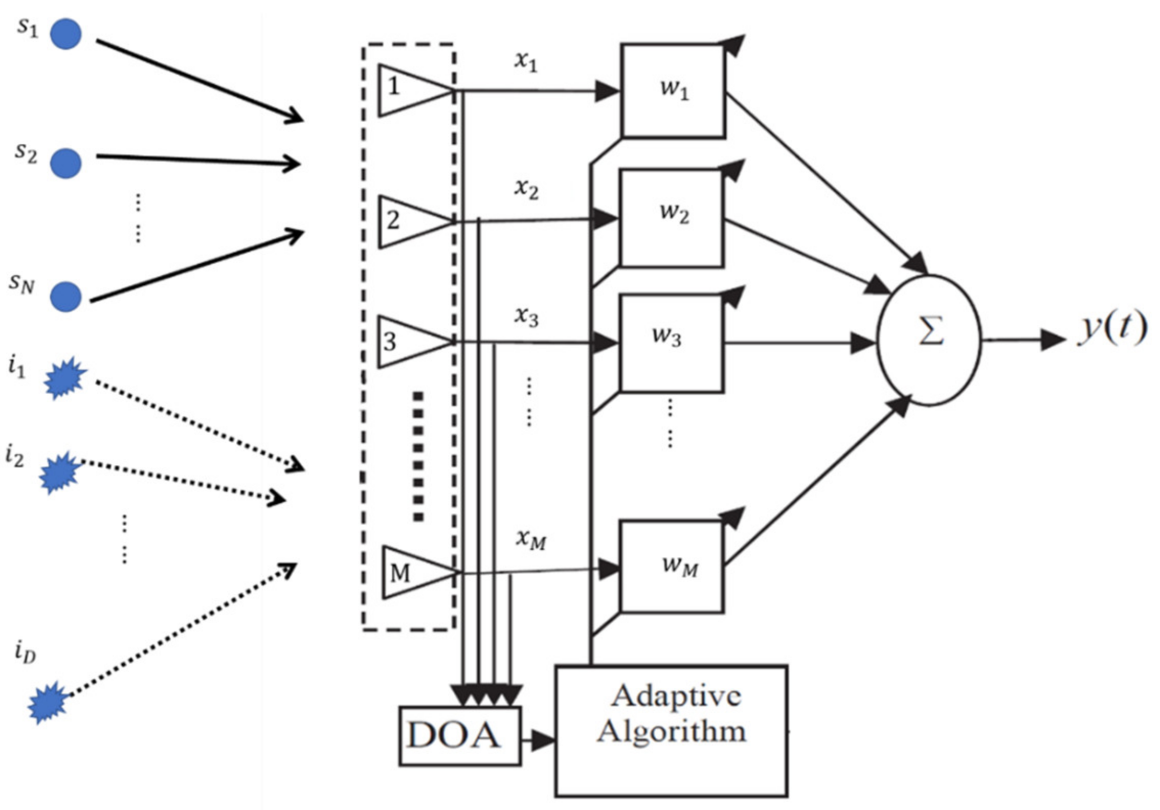
2. Adaptive Antenna Array Signal Model

Consider there is an antenna array made up of $M$ elements that receive $N$ desired signals (i.e., $s_1\cdots \cdots s_N$) and $D$ interference signals (i.e., $i_1\cdots \cdots i_D$) from different directions shown in Figure 1. As a result, the signal induced on all elements can be given in terms of a vector notation:

$$\mathit{x}\left(t\right)={{\displaystyle \sum }}_{k=1}^N{\mathit{s}}_{\mathit{k}}\left(t\right){\mathit{a}}_N\left({\theta }_k\right)+{{\displaystyle \sum }}_{l=1}^D{\mathit{i}}_l\left(t\right){\mathit{a}}_D\left({\theta }_l\right)+\mathit{n}\left(t\right), t=1, 2, \dots .T$$

(1)

In this case, ${\mathit{s}}_{\mathit{k}}\left(t\right)$ and $\mathit{a}\left({\theta }_k\right)$ represent the kth wanted signal and the corresponding steering vector, respectively, whereas ${\mathit{i}}_l\left(t\right)$ and $\mathit{a}\left({\theta }_l\right)$ denote the lth interferes user and its steering vector, respectively. The symbol $\mathit{n}\left(t\right)$ refers to the Additive White Gaussian Noise (AWGN), while $T$ is the number of snapshots for data collection. Alternatively, the formula above can be expressed as follows:

$$\mathit{x}\left(t\right)=\mathit{s}\left(t\right)+\mathit{i}\left(t\right)+\mathit{n}\left(t\right)=\mathit{s}\left(t\right)+\mathit{u}\left(t\right)$$

(2)

Here, $\mathit{s}\left(t\right)={\mathit{s}}_k\left(t\right) {\mathit{a}}_N\left({\theta }_k\right)\in {ℂ}^{1\times M}$ and $\mathit{i}\left(t\right)={\mathit{i}}_l\left(t\right){\mathit{a}}_D\left({\theta }_l\right)\in {ℂ}^{1\times M}$ represent the received vector data of the desired and interference signals, respectively, and $\mathit{u}\left(t\right)$ refers to the unwanted signal (i.e., interference signal + noise) vector at the receiver end, while $\mathit{x}\left(t\right)\in {ℂ}^{1\times M}$ is the total received data vector that contains all the previously mentioned signals.

The covariance matrix of the wanted and interference signals, in addition to the additive noise, is constructed as follows [11]:

$${{ℛ}}_{\mathit{s}\mathit{s} }= E\left[ \mathit{s}\left(t\right) \mathit{s}{\left(t\right)}^H\right]$$

(3)

$${{ℛ}}_{\mathit{i}\mathit{i}}= E\left[ \mathit{i}\left(t\right) \mathit{i}{\left(t\right)}^H\right]$$

(4)

$${{ℛ}}_{\mathit{n}\mathit{n}}= E\left[ \mathit{n}\left(t\right) \mathit{n}{\left(t\right)}^H\right]$$

(5)

By supposing all signals are independent and the noise has a zero-mean stationary process, then the output of the receiving array, $\mathit{y}\left(t\right)$, can be formed by multiplying the computed weights, $\mathit{w}={\left[w_1 w_2 \dots \dots \dots w_M\right]}^{\mathit{T}}$, with total received signal, $\mathit{x}\left(t\right)$, yields:

$$\mathit{y}\left(t\right)={\mathit{w}}^{\mathit{H}} \mathit{x}\left(t\right)=\mathit{w} \left(\mathit{s}\left(t\right)+\mathit{i}\left(t\right)+\mathit{n}\left(t\right)\right)={\mathit{y}}_{\mathit{s}}\left(t\right)+{\mathit{y}}_{\mathit{i}}\left(t\right)+{\mathit{y}}_{\mathit{n}}\left(t\right)$$

(6)

The first element of a uniform linear array is considered to be a reference, and thus the array steering vector becomes as follows:

$$\mathit{a}\left(\theta \right)=\left[\begin{array}{ccc}1& e^{-j\beta dsin\theta }& \begin{array}{cc}\dots & e^{j\beta d\left(M-1\right)sin\theta }\end{array}\end{array}\right]$$

(7)

Here, $d$ represents the separation distance between adjacent elements, and $\beta$ is the propagation constant. To model the steering vector, which contains the information of elevation angle (i.e., $\theta$) and azimuth angle (i.e., $\varphi$), an M₁ × M₂ planar array is supposed to be located in the x–y plane. M₁ and M₂ are the antenna element numbers in the x and y directions, respectively. The steering vector of the planar antenna array needs to be computed to produce a beam towards the desired signal as follows:

$$\mathit{a}\left(\theta ,\varphi \right)={\mathit{a}}_{\mathit{x}}\left(\theta ,\varphi \right) {\mathit{a}}_{\mathit{y}}\left(\theta ,\varphi \right)$$

(8)

Here, ${\mathit{a}}_{\mathit{x}}\left(\theta ,\varphi \right)$ represents the steering vector in the horizontal plane, while ${\mathit{a}}_{\mathit{y}}\left(\theta ,\varphi \right)$ is the steering vector in the vertical direction, and it can be defined using the following formula:

$${\mathit{a}}_{\mathit{x}}\left(\theta ,\varphi \right)= {\displaystyle \sum }_{m=1}^{M_1}{e}^{j\left(m-1\right){\beta }_x}$$

(9)

$${\mathit{a}}_{\mathit{y}}\left(\theta ,\varphi \right)= {\displaystyle \sum }_{n=1}^{M_2}{e}^{j\left(n-1\right){\beta }_y}$$

(10)

where ${\beta }_x$ is the phase increment per element in the x-direction while ${\beta }_y$ represents the phase increment per element in the y-direction, and it can be defined as described below:

$${\beta }_x=\frac{\pi d_x}{\lambda }\left(sin\theta cos\varphi -sin{\theta }_{0}cos{\varphi }_0\right)$$

(11)

$${\beta }_y=\frac{\pi d_y}{\lambda }\left(sin\theta cos\varphi -sin{\theta }_{0}sin{\varphi }_0\right)$$

(12)

Finally, the manifold array vector is given by multiplying ${\mathit{a}}_{\mathit{x}}\left(\theta ,\varphi \right)$ with ${\mathit{a}}_{\mathit{y}}\left(\theta ,\varphi \right)$ as follows [11]:

$$\mathit{a}\left(\theta ,\varphi \right)={\displaystyle \sum }_{m=1}^{M_1}{\displaystyle \sum }_{n=1}^{M_2}{e}^{j\left( m-1\right){\beta }_x}{e}^{j\left( n-1\right){\beta }_y}$$

(13)

where $\lambda$ is the wavelength while $d_x$ and $d_y$ are the separation distances between the adjacent elements of the antenna array in the x and y planes, respectively.

3. The Proposed Circular Patch Antenna

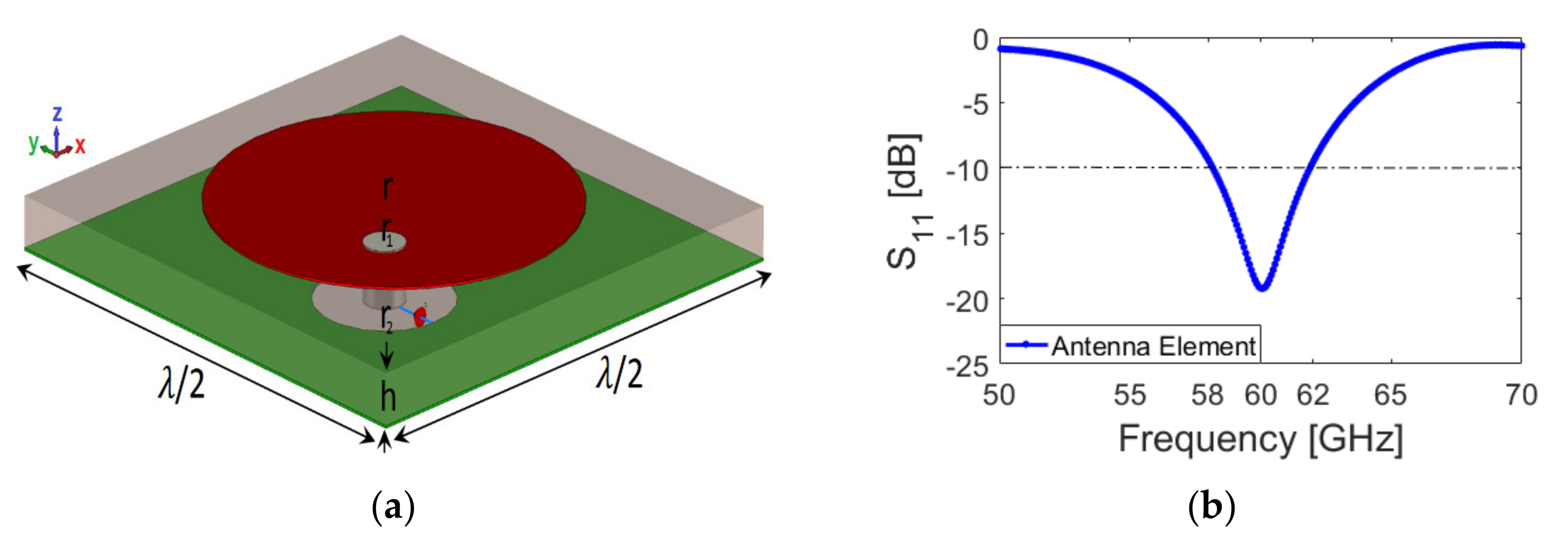
For the front-end stage, the performance of the sensor/antenna strongly affects the wireless communication link and system quality. Thus, a compact-size patch antenna with a circular shape is designed to work at a resonant frequency of 60 GHz, as illustrated in Figure 2a. An RT5880 dielectric is used in the patch antenna design with an overall size of 0.5λ × 0.5λ × h = 2.5 × 2.5 × 0.2 mm³. As shown in the figure below, the inner conductor of a coaxial cable has been brought through the substrate and connected to the circular patch surface to feed the antenna.

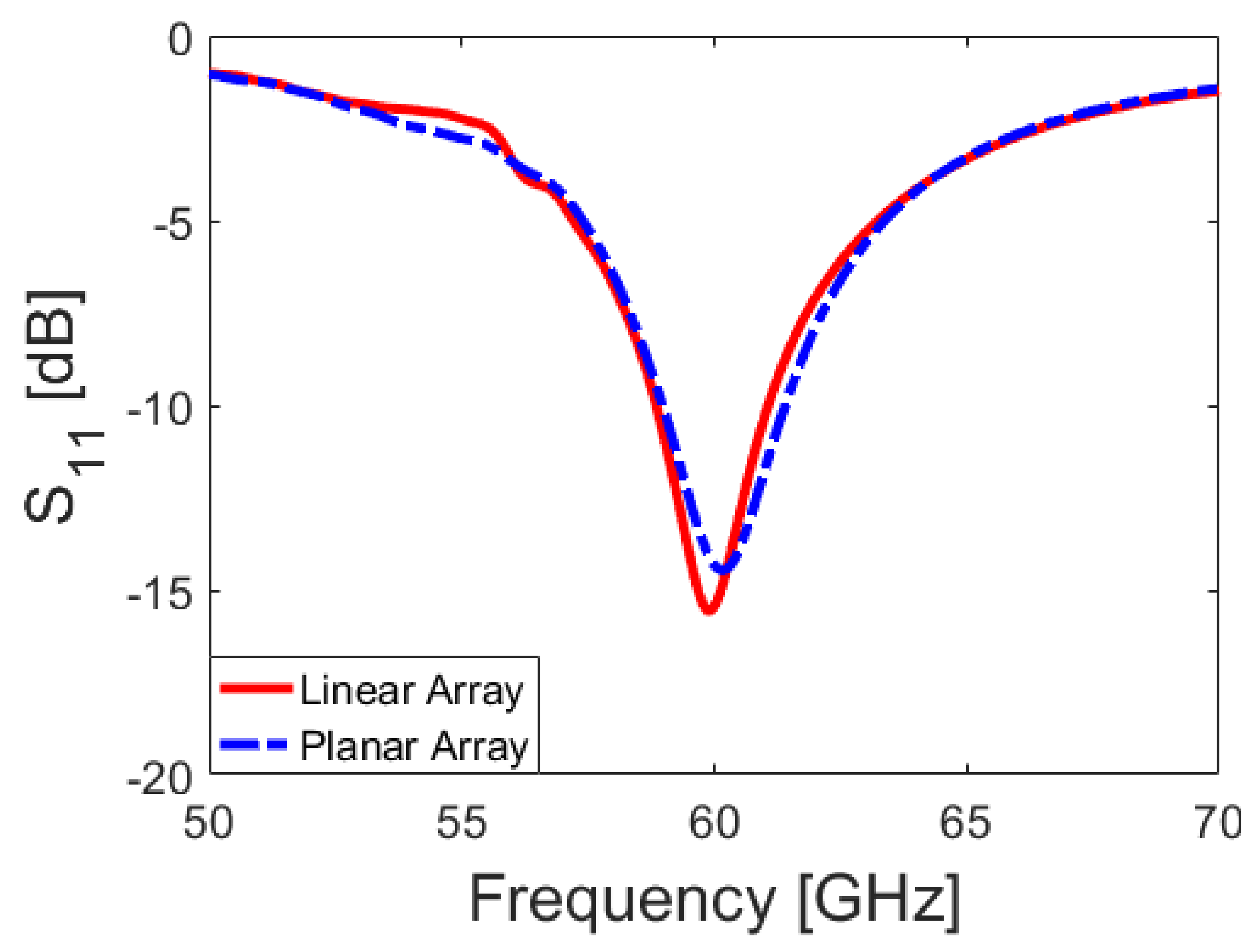
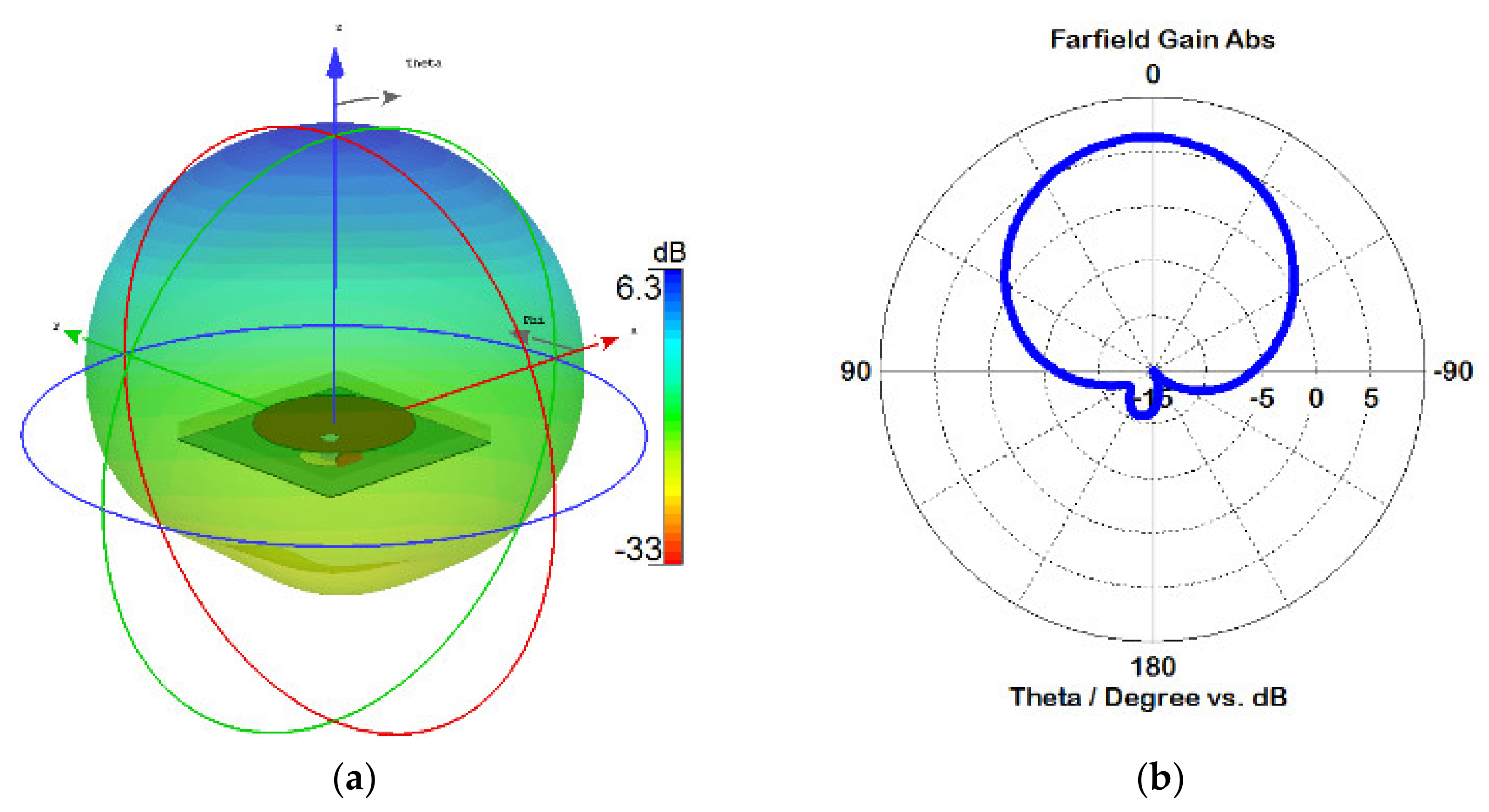
The values of the designed parameters for the proposed single-antenna element are: r (radius of the circular patch) = 0.92 mm; r₁ (radius of the inner connector) = 0.1 mm; r₂ (radius of the outer connector) = 0.35 mm; and h (substrate thickness) = 0.2 mm. The diameter of the circular patch is 0.92 × 2 = 1.84 mm, printed on a substrate with a size of λ/4 = 2.5 mm. Figure 2b illustrates the S₁₁ (i.e., the reflection coefficient) of the proposed antenna against the frequency band. As illustrated, the antenna has a 4 GHz bandwidth of around 60 GHz. The proposed antenna’s 3D and 2D radiation patterns are simulated and illustrated in Figure 3. It has low back-lobes with 7.43 dBi directivity. 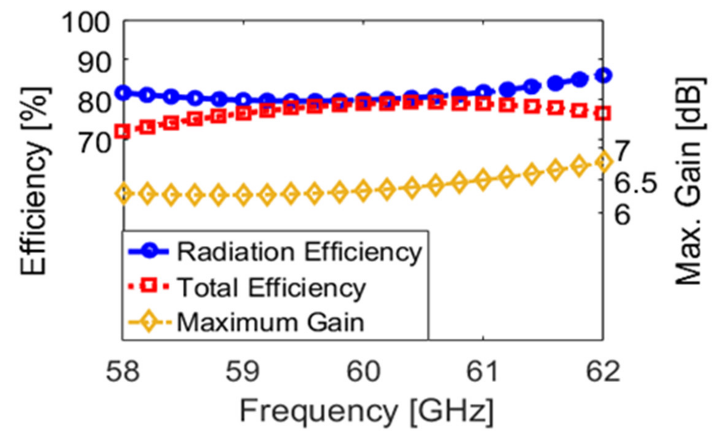Figure 4 shows the antenna efficiencies within a frequency range from 58 to 62 GHz. As shown, the designed coaxial-fed antenna has a radiation efficiency of more than 80%, and the total efficiency is higher than 70% and provides a 6.5 dB maximum gain.

Antenna array has several proven benefits in cellular systems base stations, such as increasing the channel capacity and spectrum efficiency arising from extended range coverage co-channel interference reduction [28]. Thus, it is considered an essential part of accomplishing beamforming, beam-steering, and null steering technologies. Moreover, the multipath fading reduction and isolation of signals with different AoAs as the essential property can be achieved by exploiting antenna arrays [29,30,31]. To this end, two different array configurations are designed and adopted in this work to achieve the mentioned targets. Thus, multiple elements of the proposed 60 GHz patch antenna, 1 × 32 and 8 × 8 arrays, are designed and studied where the distance between the antenna elements is set to d_x = d_y = λ/2 = 2.5 mm. 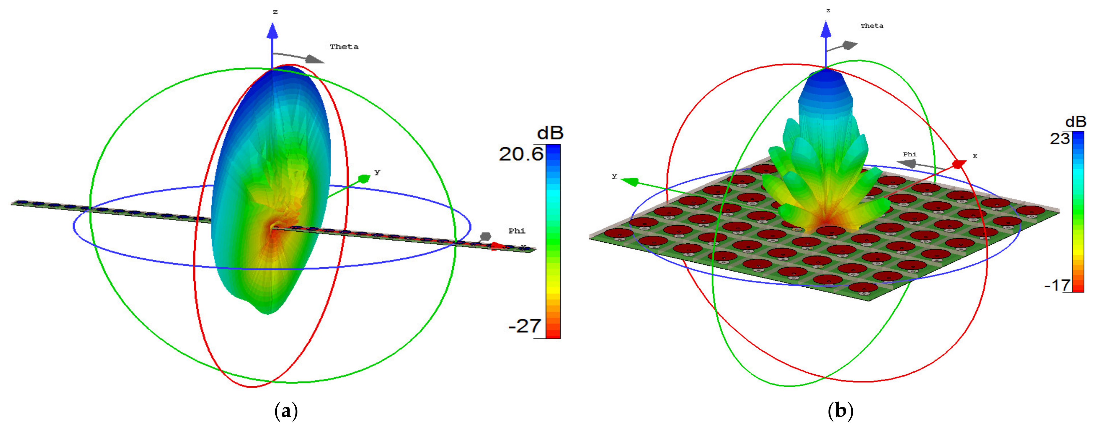Figure 5 depicts the performance of 32 linear and 8 × 8 planar arrays of the 60 GHz patch antenna.

The 3D radiation beam pattern of the 32 linear antenna array at θ = 0° and ϕ = 0° is illustrated in Figure 5a, while the 3D radiation beam pattern of the 8 × 8 planar array at directions at θ = 0° and ϕ = 90° is shown in Figure 5b. Obviously, the designed array has good beam steering characteristics with a wide range of beam-coverage properties. The obtained gains of the main beams using 32 linear arrays and 64 planar arrays are 20.6 dB and 23 dB, respectively, as shown in Figure 5.

The S₁₁ results of linear and planar antenna arrays are depicted in Figure 6. As shown, the arrays provide sufficient reflection coefficients at the desired frequency (60 GHz). However, there is a slight difference with the single-element result, mainly due to the couplings between the array elements.

The advantage of the proposed antenna is its highly compact size, and it provides desirable characteristics at 60 GHz. In addition, the antenna element provides excellent radiation performance with very low side and back lobes, which makes it a good choice for beam-steering and beamforming. The proposed patch antenna exhibits high gain levels, good radiation, and total efficiencies compared with other antenna types such as slot, monopole, etc. As shown in Figure 5, the designed linear and planar arrays provide symmetrical high-gain radiation, a flexible and wide scanning function, and narrow beamwidth, which can be used in point-to-point 5G communications.

4. The Proposed Beamforming Algorithm

The usefulness of adaptive digital beamforming stems from its capacity to compute weights that may be supplied to the antenna array elements to produce the desired radiation pattern that enhances user reception while rejecting jamming and interference signals [10]. To this end, 32 linear arrays and 8 × 8 planar arrays should be combined with an efficient beamforming method to make multiple adaptive beams and nulls. To this end, we propose a new-efficient adaptive beamforming algorithm that relies upon estimating the maximum likelihood of the desired signal power, while the rest of the signals are assumed to be interference sources. The signal to interference (SIR) ratio can be represented as follows:

$$SIR=\frac{P_s}{P_i}$$

(14)

where $P_s$ and $P_i$ are the received power of the desired and interference signals, respectively.

Let us assume a beam needs to be produced towards the desired user in order to improve its reception, while the rest of the directions are supposed to be interference or unwanted sources. Thus, the downlink channel’s noise/unwanted correlation matrix needs to be measured. It may be difficult to separate signal/interference from noise in practical applications. However, it is possible to separate the inclusion of the signal from the interference and noise covariance matrix if the desired direction is known by applying a cross-correlation technique between the received signal and such a pilot signal. Once the desired signal is extracted, the rest of the signal will be treated as noise necessary for the next stage of the beamforming process. However, the method does not involve the interference directions in the computation engine of the array weights. Consider the observed noise correlation matrix, ${{ℛ}}_{\mathit{n}\mathit{n} }\in {ℂ}^{M\times M}$, as follows:

$${{ℛ}}_{\mathit{n}\mathit{n} }= \left(\begin{array}{ccccc}{𝓇}_{1,1}& {𝓇}_{1,2}& \dots & {𝓇}_{1,M-1}& {𝓇}_{1,M}\\ {𝓇}_{2,1}& {𝓇}_{2,2}& \dots & {𝓇}_{2,M-1}& {𝓇}_{2,M}\\ ⋮& ⋮& \ddots & ⋮& ⋮\\ {𝓇}_{M,1}& {𝓇}_{M,2}& \dots & {𝓇}_{M,M-1}& {𝓇}_{M,M}\end{array}\right)$$

(15)

Once this goal is achieved, the next step is to sample $N$ columns (i.e., the number of desired users) from the measured noise correlation matrix to construct the projection noise matrix. The challenge here is how to sample the $N$ columns in such a way that can provide the best representation of the original matrix (i.e., ${{ℛ}}_{\mathit{n}\mathit{n}}$) and extract the information about the signal parameters efficiently [32,33,34]. To this end, assume ${\mathit{Q}}_N$ represents the sampled matrix constructed by sampling N columns uniformly instead of sampling the first N columns straightforwardly. It should be noted that the proposed sampling methodology sampled the first and last columns deliberately to maximise the aperture size of the sampled matrix, while the rest of the columns were sampled based on the following formula:

$$\kappa =\left\{k_i|k_i=round\left(\frac{\left(i-1\right)·M}{\left(N-1\right)}\right) \mathrm{for} i=\left\{2,\dots ,N-1\right\}\right\}$$

(16)

where $\kappa ={\kappa }_i|{\kappa }_i$ represents the number of the selected random column in the set and can be expressed as given below:

Then, the total sampled matrix, including the first and last column, can be expressed as follows:

$${\mathit{Q}}_N=\left(\left\{\begin{array}{c}\begin{array}{c}{r}_{11}\\ r_{21}\end{array}\\ ⋮\\ r_{M1}\end{array}\right\} \left\{\begin{array}{ccc}{r}_{1\kappa }& \dots & r_{1\kappa }\\ r_{2\kappa }& ⋮& r_{2\kappa }\\ ⋮& \ddots & ⋮\\ r_{M\kappa }& \dots & r_{M\kappa }\end{array} \right\} \left\{\begin{array}{c}\begin{array}{c}{r}_{1M}\\ r_{2M}\end{array}\\ ⋮\\ r_{MM}\end{array}\right\}\right)$$

(17)

Once the sampled matrix is measured, the projection matrix can be constructed using the formula below.

$${{𝒫}}_{\mathit{P}\mathit{N}\mathit{C}\mathit{M}}={\mathit{I}}_{\mathit{M}}- {\mathit{Q}}_N{}^{\mathit{H}} {\left({\mathit{Q}}_N {\mathit{Q}}_N{}^{\mathit{H}}\right)}^{-\mathbf{1}}{\mathit{Q}}_N$$

(18)

As can be seen from the formula above, the performance and effectiveness of ${{𝒫}}_{\mathit{P}\mathit{N}\mathit{C}\mathit{M}}$ depends mainly on ${\mathit{Q}}_N$. Now, to compute such optimum weights, the Joint Probability Density Function (JPDF) is applied to estimate the measured parameter, $\mathit{n}=\mathit{x}- {\mathit{a}}_{\mathit{N}}\left(\theta ,\varphi \right)\mathit{s}$, as described below.

$$P\left(\raisebox{1ex}{$\mathit{x}$}\!\left/ \!\raisebox{-1ex}{$\mathit{s}$}\right.\right)=\frac{1}{\sqrt{2\pi {\sigma }_n^2}}\exp -\left\{{\left(\mathit{x}- {\mathit{a}}_{\mathit{N}}\left(\theta ,\varphi \right)\mathit{s}\right)}^H {{𝒫}}_{\mathit{P}\mathit{N}\mathit{C}\mathit{M}} \left(\mathit{x}- {\mathit{a}}_{\mathit{N}}\left(\theta ,\varphi \right)\mathit{s}\right)\right\}$$

(19)

Since the wanted signal is placed in the exponent part of the equation above, a log function is taken for both sides as follows:

$$L\left[\mathit{x}\right]=-\log \left[P\left(\raisebox{1ex}{$\mathit{x}$}\!\left/ \!\raisebox{-1ex}{$\mathit{s}$}\right.\right)\right]=C\left\{{(\mathit{x}-{\mathit{a}}_N\left(\theta ,\varphi \right)\mathit{s})}^H{{𝒫}}_{\mathit{P}\mathit{N}\mathit{C}\mathit{M}}\left(\mathit{x}-{\mathit{a}}_{\mathit{N}}\left(\theta ,\varphi \right)\mathit{s}\right)\right\}$$

(20)

where $C=-\frac{1}{\sqrt{2\pi {\sigma }_n^2}}$ is a constant.

To maximise the log-likelihood function, (i.e., $L\left[\mathit{x}\right]$) is partially derived to $\mathit{s}$ and set to zero as given below.

$$\frac{\partial L\left[\mathit{x}\right]}{\partial \mathit{s}}=-2 {\mathit{a}}_{\mathit{N}}^H\left(\theta ,\varphi \right) {{𝒫}}_{PNCM }\mathit{x}+2\mathit{s}{\mathit{a}}_{\mathit{N}}^H\left(\theta ,\varphi \right) {{𝒫}}_{PNCM }{\mathit{a}}_{\mathit{N}}\left(\theta ,\varphi \right)=0$$

(21)

Solving the equation above for $\mathit{s}$ yields:

$$\mathit{s}=\frac{{\mathit{a}}_{\mathit{N}}^H\left(\theta ,\varphi \right) {{𝒫}}_{PNCM}}{{\mathit{a}}_{\mathit{N}}^H\left(\theta ,\varphi \right){{𝒫}}_{\mathit{P}NCM} {\mathit{a}}_{\mathit{N}}\left(\theta ,\varphi \right)}\mathit{x}=\mathit{W}\mathit{x}$$

Then, the obtained optimum weights are:

$$\mathit{W}=\frac{{\mathit{a}}_{\mathit{N}}^H\left(\theta ,\varphi \right) {{𝒫}}_{PNCM}}{{\mathit{a}}_{\mathit{N}}^H\left(\theta ,\varphi \right){{𝒫}}_{\mathit{P}NCM} {\mathit{a}}_{\mathit{N}}\left(\theta ,\varphi \right)}$$

The formula above can be further simplified to be written as follows:

$$\mathit{W}={{𝒫}}_{PNCM} {\mathit{a}}_{\mathit{N}}\left(\theta ,\varphi \right)$$

(22)

It can be noticed that the optimum weights are computed without the requirement to find the correlation matrices of useful and interference signals. In addition, there is no need for matrix inverse calculation and Eigen decomposition operations, which makes the operating system more efficient than the classical beamformers.

To make the size of $\mathit{W}$ size in (22) compatible with the array steering vector size, it is possible to manipulate these matrices’ sizes by applying a summation over each column to obtain an average weight vector, ${\mathit{w}}_{\mathit{v}}=\sum \mathit{W}$, with dimensions ($M\times 1$) and (($M_1{M}_2$) $\times$ 1) for 1D and 2D arrays, respectively. The output radiation pattern can be formed by multiplying the optimum weights by the steering vector as follows:

$$AF\left(\theta ,\varphi \right)=\mathit{a}\left(\theta ,\varphi \right) {\mathit{w}}_{\mathit{v}}$$

(23)

The array factor, $AF\left(\theta ,\varphi \right)$, can be normalised as follows:

$$A{F}_{normalised }=\frac{AF\left(\theta ,\varphi \right)}{\underset{\left(\theta ,\varphi \right)}{\max }\left|\left(AF\left(\theta ,\varphi \right)\right)\right|}$$

(24)

As can be seen, the array factor is a function of the array geometry and amplitude/phase shifts applied to individual elements. It should be noted that the array steering vector depends on the exploited antenna element and the array shape, while the fed weights to the antenna array are based on many factors such as the selected beamforming method, Channel State Information (CSI) and location of desired and interference users to the receiving array, etc.

4.1. Beam Generation and Adjustment Using the PNCM Algorithm

The procedures and simulation steps for generating and directing beams toward the desired users using the proposed beamforming algorithm are summarised below.

Algorithm 1 The simulation procedures of the proposed beamforming approach.

Algorithm 1: Projection Noise Correlation Matrix
Input:	${{ℛ}}_{\mathit{n}\mathit{n} }\in C^{M\times M}$, T number of snapshots, frequency (fc) and N desired directions, M elements for 1D array and M1, M2 for a planar array
Output:	The desired output radiation pattern of the antenna array
Step 1:	Sample ${\mathit{Q}}_N$ based on the Equations (17) and (16) conditions
Step 2:	Construct the noise projection correlation matrix, ${{𝒫}}_{\mathit{P}\mathit{N}\mathit{C}\mathit{M}}$, using (18)
Step 3:	Apply JPDF to estimate $\mathit{n}=\mathit{x}- {\mathit{a}}_{\mathit{N}}\left(\theta ,\varphi \right)\mathit{s}$ using (19)
Step 4:	Set the gradient of (20) to zero and calculate the weights as given in (22)
Step 5:	Apply (23) to construct the output radiation pattern of the antenna array
Step 6:	%For the 1D array, the Array Factor (AF) is constructed in MATLAB as follows: fc = 60 × 109;    % Carrier frequency c = 3 × 108;         % Speed of light (m/s) lambda = c/fc;      % wavelength d = lambda/2;      % Inter element spacing theta = (−90 : 0.5 : 90); n = 1:M; d = 0.5; for ii = 1: length (theta) th = theta(ii) a = exp(1j×2×pi× (n − 2) ×d×sin(th×pi/180)).’; AF1(:,ii) = Wv’ ×a; end
Step 7:	%For the 2D array, AF can be constructed in MATLAB as follows: [n,m] = meshgrid(−1× (M1 − 1)/2:(M1 − 1)/2, −1× (M2 − 1)/2:(M2 −1 )/2); nn = reshape (n,[],1); mm = reshape (m,[],1); dx = 0.5; dy = 0.5; theta2 = 0 : 0.5 : 90; phi = 0 : 0.5 : 360; for ii = 1:length(theta2) for iii = 1:length(PHI) ax = 2×pi×dx×sin(theta2(ii) ×pi/180) ×cos(PHI(iii) ×pi/180); ay = 2×pi×dx×sin(theta2(ii) ×pi/180) ×sin(PHI(iii) ×pi/180); aa = exp(1j× (nn×ax + mm×ay)); AF2(ii,iii) = Wv’×aa; end end
Step 8:	Plot the output radiation pattern of the array as follows: plot (theta,20×log10(abs(AF1)/max(abs(AF1)))) %For linear array mesh (PHI,theta2, abs(AF2)/max(abs(AF2))) %For planar array

4.2. Degrees of Freedom (DOFs) Theoretical Analysis

The DOFs characteristic function is computed using the separated distances between the sampled columns to investigate the proposed distribution advantage. It should be noted that our objective here is to determine the number of nulls/maxima of the antenna array factor. Accordingly, the array factor using the classical sampling approach can be formulated using the first $N$ sampled columns as described below.

$$\mathit{A}{\mathit{F}}_{\mathit{C}}\left(\theta \right)=\left[1 e^{-j\pi \cos \theta } \dots e^{-j\left(N-1\right)\pi \cos \theta }\right]$$

(25)

The formula above can be multiplied by $e^{-j\pi \cos \theta }$, yielding:

$$\mathit{A}{\mathit{F}}_{\mathit{C}}\left(\theta \right) e^{-j\pi \cos \theta }=\left[ e^{-j\pi \cos \theta } e^{-2j\pi \cos \theta } \dots e^{-jN\pi \cos \theta }\right]$$

(26)

Equation (26) can be subtracted from Equation (25) as follows:

$$\mathit{A}{\mathit{F}}_{\mathit{C}}\left(\theta \right)=\frac{\left(e^{-jN\pi \cos \theta }-1 \right) }{\left(e^{-j\pi \cos \theta }-1\right)}$$

(27)

The formula above represents the number of nulls using the conventional sampling criterion. By performing further manipulations and simplifications, (27) becomes as follows:

$$\mathit{A}{\mathit{F}}_{\mathit{C}}\left(\theta \right)=\frac{sin\left(\frac{N\pi \cos \theta }{2}\right) }{sin\left(\frac{\pi \cos \theta }{2}\right)}$$

(28)

As can be seen, the array factor using the classical criterion produced only $N$–1 nulls, which could be used to provide beams in the wanted directions and/or put nulls in the unwanted directions. In order to formalise the investigation of the proposed beamforming method, let us define an object, X_j, which represents a column location at x point and another object, called X_k (k$\ne$j), located at the position of ‘x + U’ with no other objects located between them. Based on this assumption, the number of produced nulls is computed to verify the angular resolution of the suggested sampling methodology in comparison with the classical distribution in which the array factor can be formulated as follows:

$$\mathit{A}{\mathit{F}}_{\mathit{U}}\left(\theta \right)=\left[1 e^{-j\left(U-1\right)\pi \cos \theta } e^{-j\left(2U-1\right)\pi \cos \theta }\dots e^{-j\left(NU-1\right)\pi \cos \theta }\right]$$

(29)

Here, U = round (M/N) represents the uniform sampled factor. Both sides of the equation above are multiplied by $e^{-jU\pi \cos \theta }$ which results in:

$$\mathit{A}{\mathit{F}}_{\mathit{U}}\left(\theta \right)e^{-jU\pi \cos \theta }=\left[e^{-jU\pi \cos \theta } e^{-j\left(2U-1\right)\pi \cos \theta } \dots e^{-j\left(NU+U-1\right)\pi \cos \theta }\right]$$

(30)

By applying such a subtraction between the two above equations and after some manipulations, the result becomes as follows:

$$\mathit{A}{\mathit{F}}_{\mathit{U}}\left(\theta \right)=\frac{\left(e^{-j\mathcal{H}\pi \cos \theta }-1 \right) }{\left(e^{-jU\pi \cos \theta }-1\right)}, \mathcal{H}=\left(NU+U-1\right)$$

(31)

Alternatively, the equation above can be represented as follows:

$$\mathit{A}{\mathit{F}}_{\mathit{U}}\left(\theta \right)=\frac{\sin \left(\frac{\mathcal{H}\pi \cos \theta }{2}\right) }{\sin \left(\frac{U\pi \cos \theta }{2}\right)}$$

(32)

Based on the numerator argument of the formula above, the array factor nulls can occur at $\mathcal{H}\mathsf{\psi }$/2 = $\pm 2n\pi$ and, consequently, the produced nulls in the angular range using the proposed sampling distribution can be expressed in the following equation:

$${\theta }_{null}={\sin }^{-1}\left(\pm \frac{2n\pi }{\left(\mathcal{H}\right)}\right), n=1, 2, \dots ,\mathcal{H}$$

(33)

It can be clearly seen that the DOFs number of the Array Factor (AF) based on the proposed sampling criterion is much higher than the produced ones that sample only the first N columns of a noise correlation matrix. Therefore, to find the null ratio number, $R$, between these two criteria, the number of produced nulls in (32) is divided by (28), which yields:

$$R=\frac{A{F}_U\left(\theta \right)}{A{F}_C\left(\theta \right)}=\frac{\mathcal{H} }{\mathrm{N}-1}=\frac{NU+U-1 }{\mathrm{N}-1}$$

(34)

The null ratio number can significantly affect the beamforming process and weight generation, leading to accurate beam-steering and null steering based on the direction of the incident signals on the receiver array. Even though DOFs are equal for both approaches, the accuracy can be improved through the unique generated weights.

4.3. Computational Complexity Comparison

This section investigates the amount of the needed computation by the beamforming method to obtain the weights of an antenna array. First, it should be noted that computing matrix inversion or decomposing matrix is a complex process and needs a significant memory storage size. The computational load to perform a matrix inverse or decomposition with (M × M) dimension is $\mathsf{O} \left({\mathrm{M}}^3\right)$. Hence, these operations will make the system complex in terms of the algorithm implementation on the Field-Programmable Gate Array (FPGA) platform or System on Chip (SoC). Secondly, performing these matrices processes under poor channel conditions such as low SNR, fewer snapshots, and a high correlation between the received signals could lead to matrix singularity. Finally, the consumption power is based mainly on the running time and computational burden. Furthermore, considering many parameters such as signal and interference correlation matrices through the weights calculation process will increase the computational load.

To this end, the proposed beamforming is compared with three popular beamforming methods, namely: Maximum Signal to Interference Ratio (MSIR), Minimum Mean Square Error (MMSE), and the Minimum Variance (MV), by considering the final formula of the weight calculation as given in

Table 1. Comparing the computational complexity of the proposed method with three rival techniques.

Method	MSIR	MMSE	MV	Proposed
Weight calculation Formula	$w=\frac{{{ℛ}}_{uu}^{-1} a_N\left(\theta ,\varphi \right)}{{\zeta }_{max}}$	$w={{ℛ}}_{\mathit{x}\mathit{x}}^{\mathbf{-}\mathbf{1}} a_N\left(\theta ,\varphi \right)$	$w={{ℛ}}_{\mathit{u}\mathit{u}}^{\mathbf{-}\mathbf{1}} a_N\left(\theta ,\varphi \right)$	$w={{𝒫}}_{PNCM} a_N\left(\theta ,\varphi \right)$
Computational Complexity	$3\times \mathsf{O}\left({\mathrm{M}}^3\right)$	$\mathsf{O}\left({\mathrm{M}}^3\right)$	$\mathsf{O}\left({\mathrm{M}}^3\right)$	$\mathsf{O}\left({\mathrm{M}}^2\mathrm{N}\right)$

${{ℛ}}_{\mathit{u}\mathit{u}}={{ℛ}}_{\mathit{i}\mathit{i}}+{{ℛ}}_{\mathit{n}\mathit{n}} \in {ℂ}^{M\times M}$ is the correlation matrix of the unwanted signals. ${\zeta }_{max}$ is the largest eigenvalue. ${{ℛ}}_{\mathit{x}\mathit{x}}={{ℛ}}_{\mathit{s}\mathit{s}}+{{ℛ}}_{\mathit{i}\mathit{i}}+{{ℛ}}_{\mathit{n}\mathit{n}} \in {ℂ}^{M\times M}$ is the total received correlation matrix. ${{𝒫}}_{\mathit{P}\mathit{N}\mathit{C}\mathit{M}}={\mathit{I}}_{\mathit{M}}- {\mathit{Q}}_{\mathit{N}}{}^{\mathit{H}} {\left({\mathit{Q}}_{\mathit{N}} {\mathit{Q}}_{\mathit{N}}{}^{\mathit{H}}\right)}^{\mathbf{-}\mathbf{1}}{\mathit{Q}}_{\mathit{N}} \in {ℂ}^{M\times M}$ is a projection matrix.

.

Based on these equations and definitions, the MSIR method has the highest computational burden among the compared methods because it needs to include the largest eigenvalue in the weight calculation process. To find this value, another matrix (i.e., ${ℛ}=R_{uu}^{-\mathrm{v}1} {{ℛ}}_{\mathit{s}\mathit{s}}$) should be computed first and then decomposed to determine the largest eigenvalue. Although the MMSE and MV methods need fewer arithmetic computations than the MSIR, they are still required to compute the matrix inverse of ${{ℛ}}_{\mathit{x}\mathit{x}}$ and ${{ℛ}}_{\mathit{u}\mathit{u}}$, respectively. However, the proposed beamforming method computed the optimum weights without the need to calculate the signal correlation matrix (i.e., ${{ℛ}}_{\mathit{s}\mathit{s}}$) and the interference signal correlation matrix (i.e., ${{ℛ}}_{\mathit{i}\mathit{i}}$). Moreover, the computational burden of the projection matrix is $\mathsf{O} \left(M^{2}N\right)$ where $N “M$.

5. Numerical Simulations and Discussions

A computer simulation is used to test and evaluate the performance of the proposed beamforming scheme by considering six different scenarios. Firstly, the beamforming scheme is tested using MATLAB and MICROWAVE^® STUDIO software to form several beams and point nulls towards the desired and interference sources, respectively. The second scenario is implemented by combining the proposed 8 × 8 planar antenna arrays with the new beamforming method to form and rotate 3D multiple beams. Again, both MATLAB and CST software are applied to simulate the results. In the third scenario, two numerical examples are implemented to compare the performance of the proposed approach with three popular beamforming algorithms. The fourth scenario compares the Signal to Interference Ratio (SIR) enhancement based on the different measured SNRs at the receiver end, whereas the fifth one evaluates the computation speed and execution time of the proposed beamforming approach against the MSIR, MMSE, and MV methods. Finally, the advantage of the proposed beamforming antenna array is compared with a considerable number of relevant 5G antenna arrays based on several criteria.

5.1. 2D Beams Rotation Using Linear Array

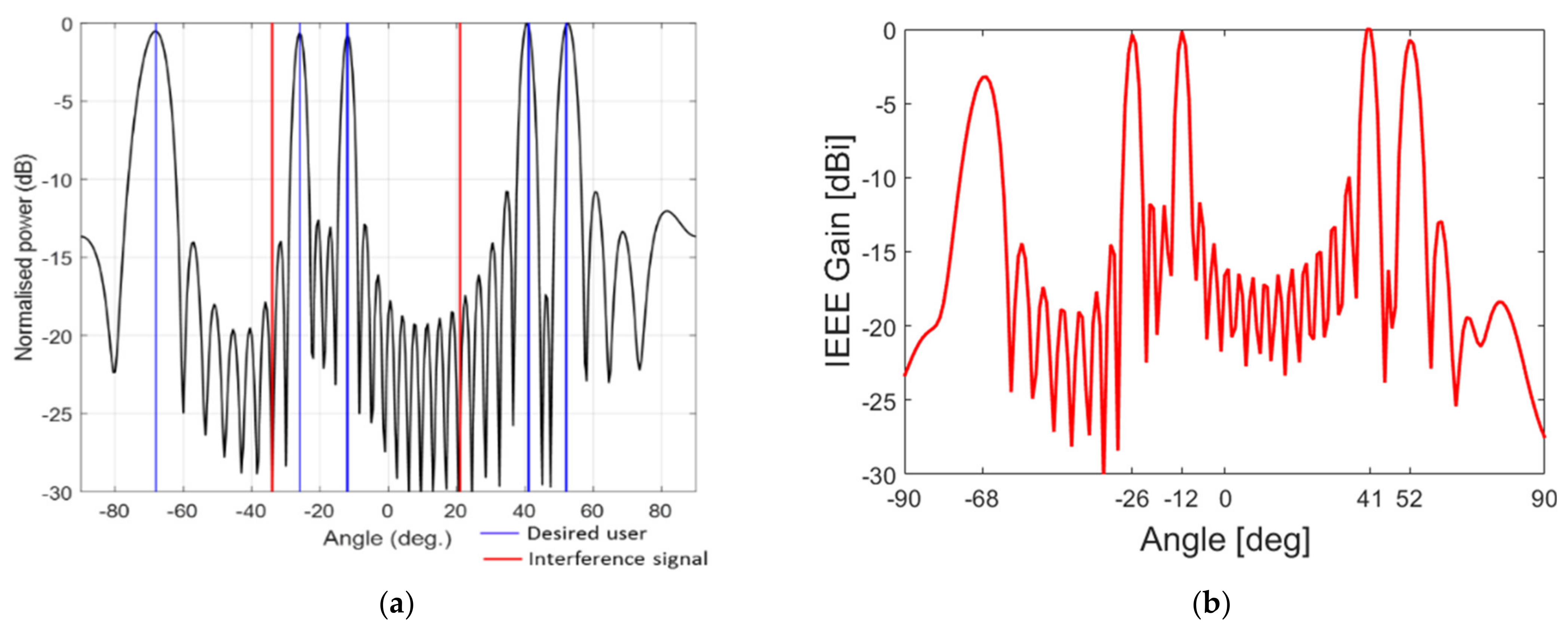
In this scenario, a 32 patch antenna element is arranged as a ULA with d = 2.5 mm and is used to enhance the channel reception of five users and reject two unwanted signals. The power of desired and inferred signals is set to be unity, while the directions of desired users and interference signals are presented in

Table 2. The directions of the desired users and interference signals.

Directions of Desired Users	Directions of Interference Signals
−68°, 41°, 52°, −12°, −26°	−35°, 21°

.

The PNCM algorithm is applied to compute the optimum weights at the baseband level (i.e., I and Q amplitudes). Then, the normalised power of the array factor is simulated using MATLAB software, as shown in Figure 7a. As shown, five beams were formed towards the desired users, while the reception of the two interference sources was rejected by putting nulls in their directions. Next, the PNCM beamforming method was used to compute the required weights and then fed manually to the 32 array elements within the CST software. As depicted in Figure 7b, five beams are produced in the directions of the desired signals, and such nulls have then formed in the unwanted locations. There is good agreement between the MATLAB and CST results, confirming that the proposed scheme works efficiently.

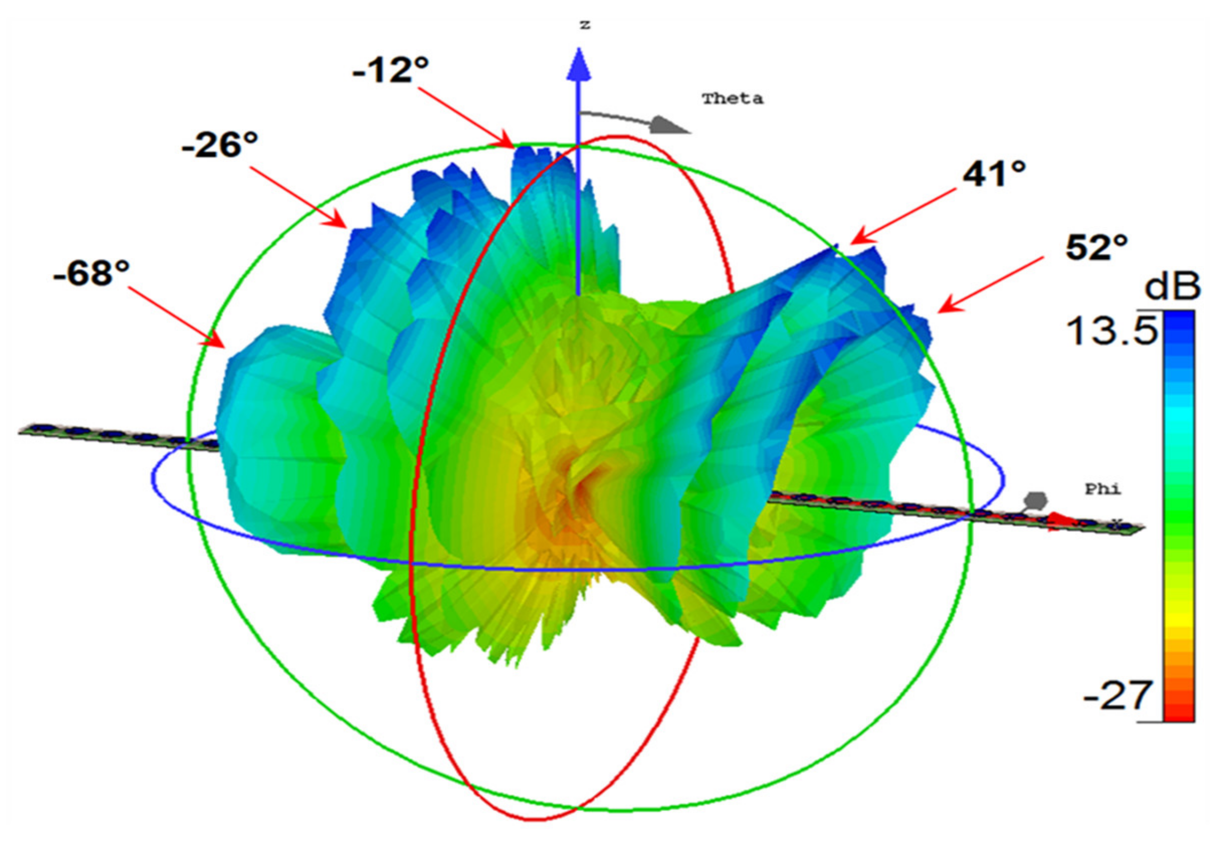
The 3D radiation patterns and the generated beams of this scenario are also simulated using CST software, as illustrated in Figure 8. This confirms that the proposed 32-linear array elements based on the new beamforming can produce multiple beams compared to Figure 5a, which generates only a single beam. Consequently, the proposed scheme has enhanced the useful users’ reception and reduced the radiated power towards the two undesired signals.

5.2. 3D Beams Rotation Using Planar Array

Despite the linear array being simple to design and fabricate, it is not suitable for three-dimensional scanning applications, such as radar systems, missile tracking, mobile communications, etc. [35]. On the other hand, the planar array appears to be a promising array configuration for military systems and wireless mobile communications networks. The beam is directed and steered in both θ and ϕ directions. To this end, this scenario simulates an 8 × 8 planar array based on the PNCM beamforming method to boost the reception of five signal sources located in the far-field with the angular locations given in

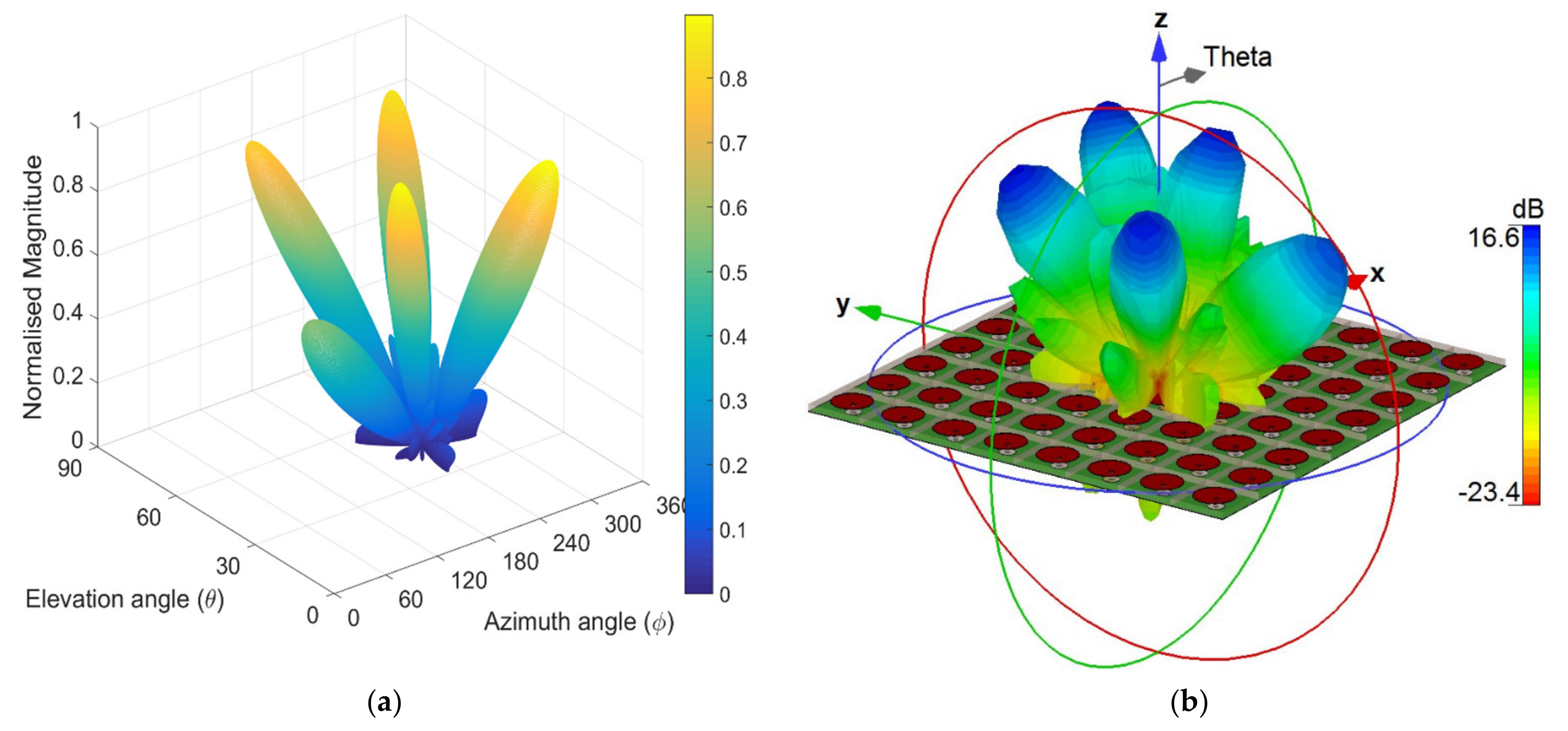
Table 3. The directions of the desired users.

User No.	1	2	3	4	5
$\left(\theta ,\varphi \right)$ in deg	(28, 327)	(32, 51)	(35, 121)	(46, 185)	(14, 192)
$\left(\theta ,\varphi \right)$ in deg	−68°, 41°, 52°, −12°, −26°		−35°, 21°

. The PNCM technique uses these angles to calculate the weights digitally, which is used to feed the planar array elements to maximise the radiated power in the directions of the wanted users by generating five beams. Therefore, about 17 dB of gain was realised for each desired user.

The 3D radiation pattern of the proposed scheme (i.e., the proposed 8 × 8 planar array in Section 3 and the proposed beamforming approach) is tested and illustrated in Figure 9. As can be observed, the proposed beamforming scheme generated five beams simultaneously toward the desired users and suppressed the reception of the other directions.

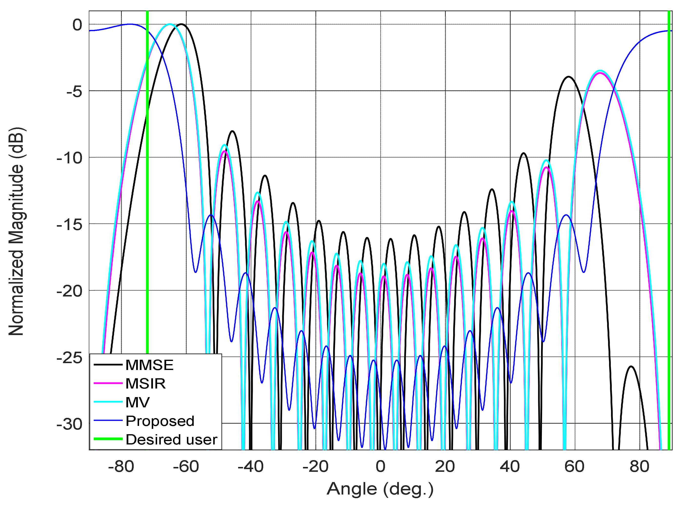
5.3. Numerical Examples Comparison

This subsection presents numerical examples of comparison between the proposed method, PNCM, and three well-known techniques, namely the MMSE method, the MSIR, and the MV method. Two scenarios are considered here to simulate such major challenges encountered by the beamformer system in practical applications. The former is to test the beamformer system performance when the directions of desired and interference signals are spatially close to each other, while the latter is to be emulated when the directions of the desired users are located near the array edges. The simulation parameters of the former and latter scenarios are given in

Table 4. The simulation parameters of the first scenario.

Parameter	M	SNR	T	Distance between Elements	Desired User Directions	Interference User Directions
Value	10	10 dB	100	$d=0.5\lambda$	${\theta }_s$ = −5°, 65°	${\theta }_I$ = −17°, 45°

and

Table 5. The simulation parameters of the second scenario.

Parameter	M	SNR	T	Distance between Elements	Directions of Desired Users
Value	16	10 dB	100	$d=0.5\lambda$	${\theta }_s$ = −72°, 88°

, respectively.

From Figure 10, it can be clearly noticed that the produced beams using the proposed method are the most accurate compared to the other compared methods. This is because the PNCM technique chooses the sampled columns uniquely, which can increase the number of DOFs and improve the antenna array weights.

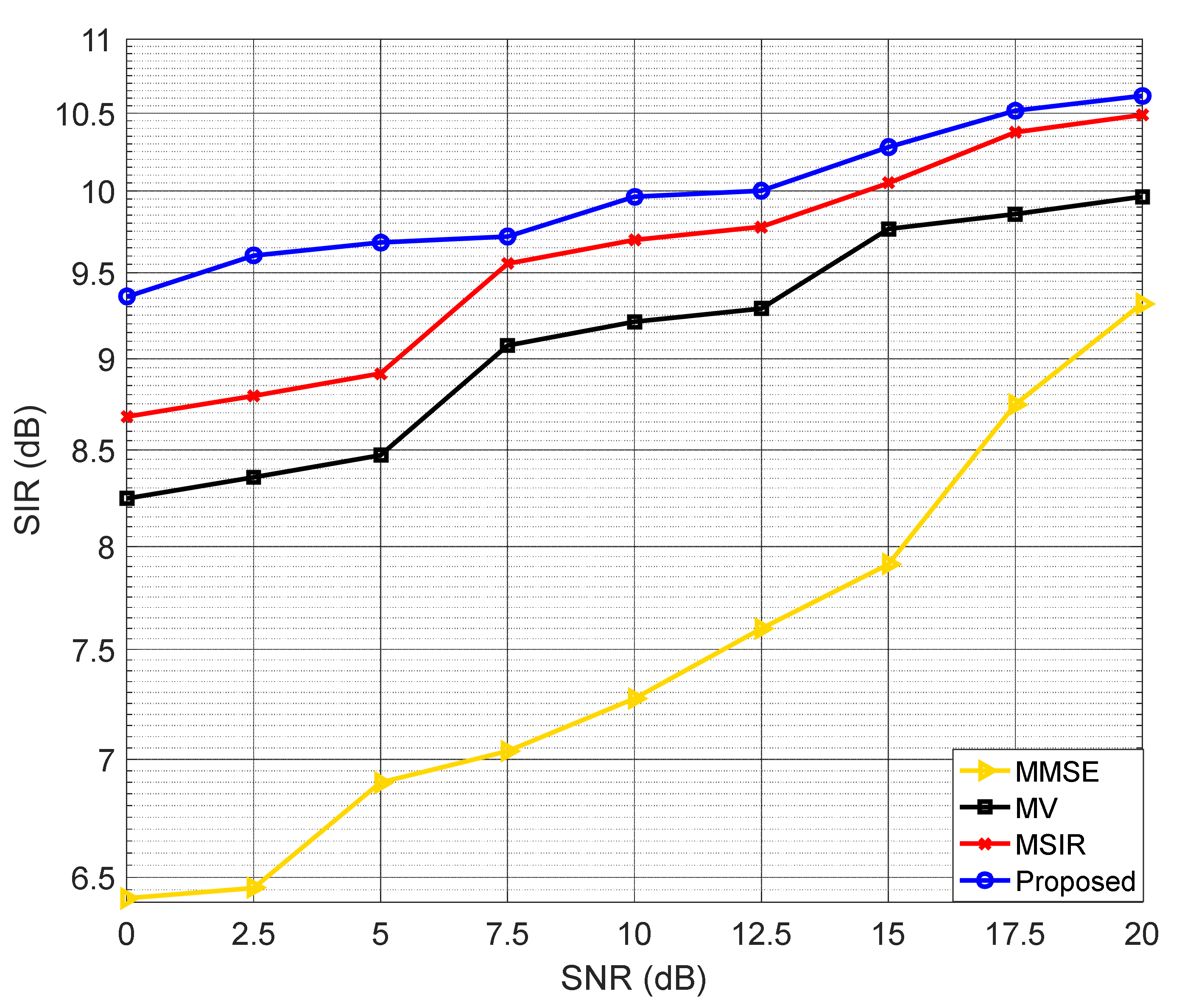
5.4. Signal to Interference Ratio (SIR) Comparison

This section compares the proposed method with the same techniques in the previous subsection based on the various values of the input SNR. A ULA made up of ten elements with a half-wavelength equally spaced between the antenna elements is considered to receive four signals. Two of them are desired while the other signals interfere. Our target is to enhance the reception in the direction of desired users while putting nulls or minimising the reception in the interference directions. The directions of all signals have been assumed to be estimated using a suitable angle of arrival method. A Monte Carlo simulation consisting of K = 1000 trials has been applied to generate the directions of the signals randomly and then passed to all the compared methods to ensure a fair comparison between them. Finally, each technique has been used to compute the required weights fed into the antenna array.

The AF of all methods is generated based on the obtained weights, and SIR is calculated to measure the method’s performance to enhance the reception of the wanted signal and reject the interference receptions via producing nulls towards them. The average SIR is computed as follows:

$$SIR=10{\log }_{10}\left(\frac{{{\displaystyle \sum }}_{n=1}^K{{\displaystyle \sum }}_{i=1}^N{P}_{si}}{{{\displaystyle \sum }}_{n=1}^K{{\displaystyle \sum }}_{j=1}^D{P}_{Ij}}\right)$$

(35)

where $K$ is the number of Monte Carlo simulations, N is the number of desired users, and D is the number of interference signals.

As shown in Figure 11, the proposed method provides the best SIR enhancement among the compared methods, which will improve the Quality of Service (QoS) of the network and the communication link between the base station and mobile stations. The interpretation of the proposed method outperforming is due to sampling and selecting that increases the physical array size and number of DOFs. As a result, the constructed projection matrix will have less between the received data and measured noise at the receiving end. Consequently, this will improve the computed weights used to generate beams in the directions of useful signal sources and put accurate nulls in the interference users’ locations.

5.5. Execution Time Comparison

The computation speed of any method is an essential part of evaluating the system efficiency and power consumption for any application. Therefore, the execution time of the PNCM approach is compared with the same techniques in the previous subsection. The same simulation parameter applied in the mentioned subsection has been assumed and used here. A simulation programme of each beamforming method was run with a for loop set to one thousand iterations (i.e. K = 1000) in MATLAB R2016–a. The average execution time has been measured using the tic and toc MATLAB functions as follows:

• tic;
• for jj = 1:K
• tstart = tic;
• Beamforming algorithm
• telapsed = toc(tstart);
• end
• averageTime = toc/K

All experiments were conducted on a computer running Windows 11 Pro, with 32 GB of installed RAM and an 11th Gen Intel (R) Core (TM) i9–11900H 2.50 GHz processor. As can be seen from the recorded execution times in

Table 6. Execution time comparison between the proposed beamforming and three different techniques.

Method	MSIR	MMSE	MV	Proposed (PNCM)
Average Execution Time	$1.3\times {10}^{-3}$	$1.2\times {10}^{-3}$	$1.1\times {10}^{-3}$	$0.88\times {10}^{-3}$
Arthemic Operations Number	3000	1000	1000	200

, the PNCM has the least execution time and needs fewer arithmetic operations than the rival methods. This advantage will make the beamforming system based on the PNCM algorithm fast and more energy efficient. These results confirm the correctness of the theoretical analysis of the computational complexity that has been conducted in Section 4.3.

It should be noted that the execution time results of the compared methods could be different from those given here according to the computer specifications and simulation situations that are associated with the programme running. Still, the behaviour of every method should be relatively the same.

5.6. Antenna Array Beamforming Comparison

A comparison with the most recent relevant works was made to demonstrate the effectiveness and advantages of the proposed beamforming antenna array. The comparison includes the frequency band, array elements and dimension, beamwidth, efficiency, the produced gain, and expected applications, as given in

Table 7. Comparison between the proposed antenna and several mm-wave antenna designs.

Refences	Frequency Band (GHz)	Array Elements	Dimension (mm)	Beamwidth (°)	Efficiency	Gain (dBi)	Applications
[36]	59.6–61.2	8 × 8	29.4 × 29.4	–30–+30	NA	22	5G base stations
[37]	58.46–62.14	4 × 1	12.8 × 10.87	±45	90%	10.02	3D AiP applications
[38]	57–66	4 × 6 (10 layers)	20 × 15	±45	NA	14.5	3D AiP applications
[39]	27.5–28.35	4 × 4	30 × 30	22	64%	16.02	Digital beamforming applications.
[40]	57.2–64.5	4 × 4 (5 layers)	14 × 14	50	89%	4.5–7.5	60–GHz-phased array
[41]	24–26	8 × 2	150 × 126	–14.6–27.9	65%	10	Future wireless devices.
[42]	57–66	1 × 1 (4 layers)	11 × 11	NA	78%	6	Industrial applications
[43]	23.34–28.25	10 × 2	79.42 × 11.53	32	70%	12.39	Future wireless devices.
[44]	55–65	4 × 16 (3 layers)	50 × 41	±50	NA	20.8	Wireless communications
[45]	27.4–28.6	4 × 4	21.2 × 19.9	–34–33	72%	10	Future wireless devices.
[46]	37.5–38.5	10 × 8	64.4 × 60	±36 and ±12	69%	19.8 and 21	High gain applications.
[47]	57.6–61.2	5 × 5	15 × 15	±40	85%	18.5	Future communication and sensing applications.
[48]	24–32	1 × 1	4.52 × 3.52	45–50	74%	10.9	Future wireless devices.
[49]	50–70	2 × 4	10.0 × 19.50	26	73%	13.4	Wi-Gig applications.
[50]	57.24–65.88	4 × 6	27.05 × 31.60	11	40%	19.26	WLAN/WPAN point to point communications.
[51]	56.25–63.25	4 × 4 (18 layers)	14.4 × 15	NA	NA	18.62	Millimetre wave applications.
[52]	57–69.4	1 × 1	30 × 30	45.10	91.2%	11.8	V-band applications.
[53]	55–65	10 × 4	47 × 13	25	60%	16.5	Millimetre wave applications.
proposed	58–62	32 × 1 8 × 8	80 × 2.5 20 × 20	12 3	80% 85%	20.6 23	5G beamforming applications.

.

As presented, the proposed beamforming antenna array provides the highest gain and the least size among the competitive rivals with comparable efficiency to refs, [37,40,42,47,52]. Furthermore, considering the array elements, the proposed beamforming method has a smaller size and a narrower beam than the other antenna array designs.

6. Conclusions

For 5G mobile communication applications, a novel effective beamforming method has been developed for two antenna array designs. A circular patch antenna operating at 60 GHz with a bandwidth of 4 GHz was proposed first, followed by two distinct array configurations that were modelled and built. The effect of mutual coupling inside the antenna array was considered throughout the evaluation. The new beamforming approach’s concept, working principle, and theoretical analysis have been described and derived. The optimal weights were calculated using the new beamforming approach, which was then fed to 32-linear and 64-planar arrays. The PNCM technique was tested using two distinct software programmes, MATLAB and CST, and the results showed that it could efficiently produce and spin many beams. Finally, the proposed beamforming has been compared with many popular beamforming techniques in terms of SIR enhancement with various values of SNR, execution time, and the required amount of computation, and the results confirmed the superiority of the PNCM method. The advantages of the proposed beamforming antenna arrays were demonstrated against numerous relevant mm-wave antenna arrays based on a wide range of criteria. As future work, it is intended to test the proposed beamforming with the 5G standards in a real-time scenario by considering measured data from a particular 5G network covering indoor and outdoor environments or using Wireless-InSite software and the 5G MATLAB toolbox to build and simulate dense urban, urban macro, and rural environments.