Article

Techno-Economic Evaluation of 5G-NSA-NPN for Networked Control Systems

1
Laboratory for Machine Tools and Production Engineering (WZL), RWTH Aachen University, Campus Boulevard 30, 52074 Aachen, Germany
2
Fraunhofer Institute for Production Technology IPT, 52074 Aachen, Germany
*
Author to whom correspondence should be addressed.
Electronics 2022, 11(11), 1736; https://doi.org/10.3390/electronics11111736
Submission received: 28 April 2022 / Revised: 20 May 2022 / Accepted: 24 May 2022 / Published: 30 May 2022
(This article belongs to the Special Issue 5G Technology in Smart Manufacturing)

Abstract

:
Wireless closed-loop control systems, so-called networked control systems (NCS) promise technical and economic benefits for production applications. To realize prospective benefits, the right communication technology is key. The fifth generation of mobile communication is predicted to have a significant impact on the deployment of NCS in the industrial connectivity landscape. However, there are different options for 5G deployment influencing both technical performance and economic aspects of the network. This in turn is expected to have a techno-economic influence on the production itself. Thus, a trade-off between the necessary technical performance of the 5G network and the benefits for the production must be executed. This paper, therefore, aims to analyze the techno-economic benefits of 5G deployment for closed-loop control systems in production. To reach this aim, first, the fundamentals of techno-economic analysis are introduced. Second, the results of an experimental performance analysis of a 5G-NSA-NPN at Fraunhofer IPT in Aachen are shown. Third, based on the results from the experimental study, a model-based techno-economic ex-ante evaluation of 5G-NSA-NPN for closed-loop applications is performed, and an exemplar is shown for a BLISK milling use case. Finally, the results are summarized and an outlook for further research is given. The analysis shows a difference in net present value for 5G deployment of EUR 2.6 M after 10 years and a difference of OPEX per product of around EUR −1000 per BLISK. Furthermore, analysis shows an increase in productivity (0.73%), quality (30.75%), and sustainability (2.87%). This indicates a noticeable improvement of a 5G-controlled NCS.

1. Introduction

In common production facilities, closed-loop control systems are often realized through wired communication [1]. However, to meet future industry demands, production systems require flexibility [2,3]. Wired communication will reach its limits and must be replaced by wireless alternatives. Wireless communication has several technical advantages: besides higher flexibility, it enables easier integration of new applications, reduces cabling efforts for large control systems, and mitigates cable breakage, to only mention some [4,5,6,7]. These technical advantages of wireless communication result in cost reduction as material cost, installation, and maintenance efforts decrease. In addition, time, labor, and materials for inspecting, testing, and upgrading wires are not necessary for wireless communication [4,8]. Therefore, networked control systems (NCS) have been, and still are, the main research focuses in academia as well as in industry.
To implement NCS in production and realize prospected benefits, the right communication technology is key [8]. From a technological point of view, communication technology must especially be reliable and fulfill latency requirements [9,10,11]. The fifth-generation (5G) of mobile communication, which is also referred to as 5G technology, is predicted to have a significant impact on the deployment of NCS in the industrial connectivity landscape, as it was developed according to the design requirements of demanding industrial control applications [12]. These technical benefits are reflected by the forecasted economic benefits of 5G in the production industry [13,14].
However, despite the expected benefits of 5G technology, the current deployment state of 5G in production companies is relatively low. A joint study by MHP and Ludwig Maximilian University shows that only 1% of companies have fully deployed 5G yet, 13% are using 5G partially [15] and 39% of companies are not planning to deploy 5G at all. The biggest barriers to 5G deployment in production according to the Digital Catapult UK manufacturing survey [16] are a lack of understanding of the return on investment (RoI), mentioned by 72%, and a lack of technical use case understanding, mentioned by 44%. Furthermore, there are different options for 5G deployment, e.g., as a public or non-public network (NPN) and standalone (SA) or non-standalone (NSA) network [17], influencing both technical performance and economic aspects of the network. This in turn is expected to have a techno-economic influence on the production itself. Thus, a trade-off between the necessary technical performance of the 5G network, its deployment cost, and the benefits for the production must be executed.
To tackle the above-mentioned barriers, this paper analyzes the techno-economic benefits of 5G deployment for NCS in production, more precisely, of a 5G-NSA-NPN. Thereby, the goal is to refer to the technical performance of 5G technology on both technical and economic performance of a closed-loop control use case in production. Figure 1 shows the structure of this paper. In Section 2, the fundamentals for this techno-economic analysis are presented. In Section 3, the results of an experimental performance analysis of a 5G-NSA-NPN at Fraunhofer IPT in Aachen are shown. Based on this technical performance, a techno-economic evaluation of 5G-NSA-NPN closed-loop applications is performed in Section 4, and an exemplar is shown for a BLISK milling use case. Section 3 and Section 4 are thereby the novelty of our research. Section 5 summarizes the results and gives an outlook for further research. This way, the paper contributes to solving the deployment barriers of 5G and increasing the worldwide GDP of production industry.

2. Fundamentals

2.1. Networked Control System

Wireless closed-loop control systems, so-called networked control systems (NCS), have been, and still are, the main research focus in academia as well as in industry [6,18]. The general working principle and components of NCS are the same as for closed-loop control systems. However, controllers, actuators, and sensors are interconnected by a communication network. This network can also be shared with other control loops, as is the case for the centralized AGV control. Different architectures of NCS exist [19,20]. Figure 2 shows the architecture as it is referred to in this paper.
In this architecture, the controller is attached to the actuator but physically separated from the sensor. The controller is stationary [22]. Sensor, controller, and actuator can either be time-driven or event-driven components. In a time-driven component, input reception or output transmission is controlled by a sampling time, which is e.g., represented by a clock signal. An event-driven component starts to process immediately at the arrival time of a component input. Communication between the components only takes place when the control difference variable e exceeds a pre-defined limit. In one NCS, all components can be time-driven, event-driven, or a mixture of both [6,20]. This depends on the control techniques used. In the further course of this paper, NCS are assumed event-driven components. To implement an NCS and profit from the advantages described in Section 1, the wireless communication network of choice must meet the strict performance requirements of process control applications. Section 2.2, therefore, explains the performance characteristics of wireless communication technologies relevant to this paper.

2.2. Performance Characteristics of Wireless Communication Technologies

2.2.1. Latency

A latency-critical application is characterized by a maximum application-perceived latency Δ t l ,   a p p l i c a t i o n ,   m a x , which must not be exceeded to ensure the functionality of the application. If Δ t l ,   a p p l i c a t i o n ,   m a x between event and action is exceeded, failures occur. The application-perceived latency in a NCS consists of its components’ latencies, as Figure 3 shows [21]. Sensor latency τ s e n s o r describes the time between an event is sensed and recorded. Controller latency τ c o n t r o l l e r expresses the time the controller requires to analyze data from the sensor and decide on a control action, which is fed back to the actuator. Actuator latency τ a c t u a t o r describes the time between the reception of the feedback variable and the start of the physical execution of the action. Network latency τ n e t w o r k describes the time the network requires to transmit the data from the sensor to the controller and from the controller to the actuator.
Network latency, therefore, occurs twice in a NCS. Equation (1) shows the composition of the application-perceived latency in a NCS as referred to in this paper:
Δ t l , application   = τ sensor + τ controller + τ actuator + τ network
As a sensor, controller and actuator have the same impact latency-wise for both centralized and decentralized AGV control, network latency is decisive when it comes to the decision of whether a communication technology is suitable for the use case. Equation (2) defines the requirement of maximum network latency.
τ network , max     Δ t l , application ,   max     τ sensor     τ controller     τ actuator

2.2.2. Jitter

Jitter of packet delay latency is a key performance in high-speed networked control systems and an important value to determine the quality of service in networks [23,24]. In terms of this paper, jitter J i + 1 will be understood as the average absolute variation of the packet’s delay, as Equation (3) defines, where T i is the latency of the i-th packet.
J i + 1 = | T i + 1     T i |
Equation (4) defines the average network jitter J network for one measurement series with n measurements.
J network = i = 1 n 1 | T i + 1   T i | n     1

2.2.3. Loss

In a packet-switched system, as it is given for 5G networks, packet loss refers to the number of packets that fail to arrive at their intended destination. In our setup, the packets using the user data protocol (UDP) get a sequence number that is extracted from the receiver for the packet loss count. Equation (5) defines the average network’s packet loss L network , where L n is the packet loss of the n-th measurement.
L network   = 1 n L n n
UDP has a very low protocol overhead and is suitable for time-sensitive applications since it has no handshake mechanism or any delays due to the retransmission of packets. Unlike connection-oriented protocols, where the communicating peers first must establish a logical or physical data connection before exchanging information, UDP uses connectionless communication. For connectionless protocols, there is no guarantee against loss, misdelivery, or out-of-sequence delivery. Therefore, any loss should be recognizable.

2.2.4. Reliability

Network R network is defined as the overall packet loss probability. Different from availability (which is from a network’s perspective) reliability and latency are the QoS required by a mobile user or mobile device in a network [25]. Since reliability is captured by transmission errors, it is calculated via the packet loss as Equation (6) shows.
R network = 1     L network

2.3. 5G-Technology Network Architecture

To create a new worldwide communication technology standard, 3GPP designed 5G New Radio (5G NR), which is an air interface or radio access technology (RAT) [26]. 5G NR can be deployed in both existing and new frequency bands and uses two frequency ranges (FR) being defined by 3GPP. FR1 covers frequencies from 410 MHz to 7125 MHz, FR2 from 24,250 MHz to 52,600 MHz. These ranges are not static and may be extended or complemented with new ranges in future 3GPP releases [26]. Table 1 gives an overview of frequency designations and a detailed division of the frequency bands into low, mid, and high bands according to Ericsson.
In contrast to previous generations of cellular networks, 5G comes with the flexibility of integrating elements of previous cellular generations in different configurations and can thus be deployed in different ways. It can be generally distinguished between non-standalone (NSA) and standalone (SA) deployment [28]. 5G-NSA networks use both 4G and 5G core networks and infrastructure. 4G core then covers existing mid bands, whereas the 5G core covers low and high bands, with mid bands optional. 5G-SA networks only use the 5G core. 5G-SA networks require a completely new deployment, however, the QoS offered by 5G-SA networks is significantly higher. 5G-SA deployments are likely to be used for latency-critical industrial use cases [27,28].
5G networks can be public and non-public. A public land mobile network (PLMN) offers mobile network services to the public and is hosted by mobile network operators (MNO). In contrast, a 5G non-public network (NPN), also known as a private network, is intended for the sole use of a private entity such as an enterprise and provides mobile network services to a clearly defined user group.
Non-public networks offer several technical advantages, such as high QoS, high network security, and accountability regarding availability, maintenance, and operation [17,29]. Therefore, the paper focuses on NPN.

3. Performance Analysis of 5G-NSA-NPN

As already explained in Section 2.3 there are two possibilities for a 5G NPN architecture. The SA architecture, which is completely based on 5G components, and the NSA architecture, which uses the 4G core in conjunction with the 5G Radio Access Network (5G RAN) and 5G New Radio (5G NR) Interface. SA promises a significantly higher QoS of the network. However, NSA is currently easier and faster to implement since it is falling back on the 4G Core infrastructure and thus existing hardware. In order to prove whether an NSA network has similar performance characteristics as defined by ITU [30] and provides a suitable QoS as SA networks, this section analyses the 5G-NSA-NPN performance. First, Section 3.1 describes the experimental setup and test methods used for the network performance analysis. Second, Section 3.2 shows the results of the performance analysis of 5G-NSA-NPN.

3.1. Experimental Setup and Test Methods

The experimental validation is conducted in the indoor 5G-NSA-NPN at the shopfloor of Fraunhofer IPT. The bandwidth of 100 MHz covers the frequency range from 3.7 to 3.8 GHz which is available in Germany since the end of 2019 for a private licensed spectrum. As 5G User Equipment (UE), two prototype routers from Wistron NeWeb Corporation (WNC) are used. The routers are configured into bridge mode, keeping all devices in the same network. For the client-side a RaspberryPi3 is connected via ethernet to the first WNC router. On the server-side a Linux laptop is connected via ethernet to the second WNC router. As Figure 4 shows, the communication path goes from the client via the 5G base station to the server, representing a D2D communication via 5G. The setup focused on the pure communication path via 5G, whereby no other components such as sensors, clouds, or control units, that can be integrated into a closed-loop, are involved.
For the determination of the 5G latency and jitter, two different test methods were applied, the ping test (1) and the Hawkeye test (2).
The ping test defines the speed of a connection and is executed on the IP Layer, which is the network layer of the connection. For the ping test, packet size (50 Byte), test duration (600 s), and receivers IP are defined on the Linux laptop. The results are stored in a csv file for analysis. Since the ping test provides a Round-Trip Time (RTT) value for latency and jitter ( 2   ×   τ network ), the results were divided by two for estimating the one-way latency and one-way jitter as applicable for a closed-loop.
In 5G networks the uplink and downlink characteristics do not need to be alike. For this setup, we cover each time uplink and downlink both ways, whereby the balancing of the RTT values is justified.
In parallel to the ping test, a Hawkeye test was conducted. Hawkeye is a special network testing software from Keysight Technologies, which has distributed software agents on the end devices and therefore is able to measure different points in a 5G communication path. It operates on the transport layer, using the transmission control protocol (TCP), and therefore is one layer above the ping test according to the OSI model. For our setup, one software agent is installed on the Raspberry Pi (software agent 1), and the other one is on the Linux laptop (software agent 2). For the latency and jitter measurements, a bidirectional KPI test was selected. This test sends data packages of 100 kbps and 50 packets per second TCP. The test duration was identical to the ping test (600 s).
For reliability measurements, the so-called iperf3-tests were used. Iperf3 is an open tool for active measurements on IP networks. It uses a server-client model to achieve the bandwidth, packet loss, and other parameters. For our measurements, we focused on the packet loss to infer the reliability of the network.

3.2. Experimental Results

Table 2 shows the results of latency and jitter for each ten ping test and Hawkeye test measurements.
The global average of the one-way latency for the ping in 5G-NSA is 11.087 ms. The TCP packages from Hawkeye test have a global one-way “from → to” latency value of 11.901 ms, and “to → from” latency value of 11.890 ms. This results in a relatively small difference of about 0.8 ms between the IP layer and TCP layer transmission. The values justify the halving of the RTT due to the fact, that the bidirectional results from Hawkeye are almost equal. Figure 5 and Figure 6 visualize the results for the average one-way latency and jitter respectively. The blue line represents the ping latency values, the grey and orange one the Hawkeye measurements. The ping average values are in the range of 10.95 ms to 11.22 ms. Therefore, the average varies by 0.27 ms. The Hawkeye average latency values vary by 0.73 ms, from 11.60 ms to 12.33 ms. Looking at the single measurements of ping and Hawkeye, the maximum variation of the highest to the lowest latency value is 13.34 ms for ping and 14 ms for Hawkeye. The TCP Hawkeye latency values are always higher than the ping values. The average jitter is 1.9 ms on the IP level (ping test) and around 1.1 to 1.3 ms on the transport layer (Hawkeye measurements). The average jitter for TCP measurements is lower than the average jitter for the ping tests.
To measure the reliability of the 5G-NSA network, and thus loss according to Equation (5), iperf3 tests were conducted. Therefore, two laptops were connected to the WNC routers. One represents the iperf3 server, and the other one represents the iperf3 client. The iperf3 tests were executed with the following parameters duration of 120, a data rate of 1000 kbps, a packet size of 100 bytes, and UDP protocol. The test was repeated ten times. Table 3 shows the loss and reliability of NSA of iperf3 tests with UDP.
Figure 7 shows the reliability values of the 5G-NSA iperf3 test compared with the theoretical reliability values for 5G (theoretical reliability value: 99.999%):
Table 4 summarizes the experimental test results and compares them—if defined—to the nominal value according to ITU specifications. The deviation of latency between the measured mean value at IPT is currently relatively large compared to the nominal value of ITU specifications. The reason for this lies in the release of the 5G network being deployed at IPT, which is of Release 15. However, in Release 15, no ultra-reliable and low latency (URLLC) features are considered yet, thus communication is not yet deterministic. The implementation of low latency features is first planned for Release 16 [31]. However, the measured latencies of IPT NSA-NPN are significantly lower than 4G/LTE values; the maximum latency of the conducted measurements is below 21 ms, which is less than half the latency of the nominal 4G/LTE latency (50 ms). With this latency, NSA-NPN at IPT is suitable for most industrial control loops [32], however, not for the latency-critical use cases below 20 ms. For loss and thus reliability, experimental values nearly correspond to the nominal values. The largest deviation was considered for sample 8 (cf. Table 3), where measured reliability is 99.9953%. This is a deviation of 0.0037% from the nominal reliability of 99.999%.
Despite these promising values, two questions are still not answered yet: first, whether 5G-NSA-NPN has a positive impact on wireless closed-loop applications, and second, whether even these small deviations (cf. Table 4) might affect the performance of the application with the 5G-enabled NCS.

4. Evaluation of 5G-NSA-NPN for Closed-Loop BLISK Milling Process

To answer the two open questions from the end of the previous section, the five-step evaluation model developed in [33] will be applied to a BLISK milling process. This evaluation model is not specifically developed for a BLISK milling process, but to evaluate the potential of 5G for latency-critical applications in production. Thus, the model is further specified for the BLISK milling use case in this paper. Therefore, Section 4.1 specifies the evaluation model for the BLISK milling process is presented. In Section 4.2, the impact of 5G-NSA-NPN on the BLISK milling process will be shown.

4.1. Approach for Techno-Economic Evaluation

According to [33], the techno-economic evaluation is executed in five steps, as Figure 8 shows. In the first step (Application Specification, Section 4.2.1) the milling machine producing BLISKs is specified. In the second step (5G-Deployment Goal Selection, Section 4.2.2), technical and economic goals are chosen out of pre-defined goals. In the third step (5G-Control Task Selection, Section 4.2.3), the control tasks of NCS are further specified. This step especially combines the network characteristics with the application’s performance. In the fourth step (Data Entry, Section 4.2.4), necessary evaluation data will be identified based on the previous steps and entered for the evaluation. In the fifth and last step (Goal Evaluation, Section 4.2.5), selected technical and economic goals are evaluated.
The core of the research is Step 3. Besides [34], no research has evaluated the use-case benefits of 5G technology based on improvements on the control-loop level. Since the BLISK use case and the AGV use case in [34] differ widely, Section 4.2.3 of this paper is thus a core element. Steps 1, 2, and 5 were adapted based on [33,35], and Step 4 is a result of the previous three steps. The research is thereby conducted based on a literature study as well as based on the presented experimental values of Section 3.

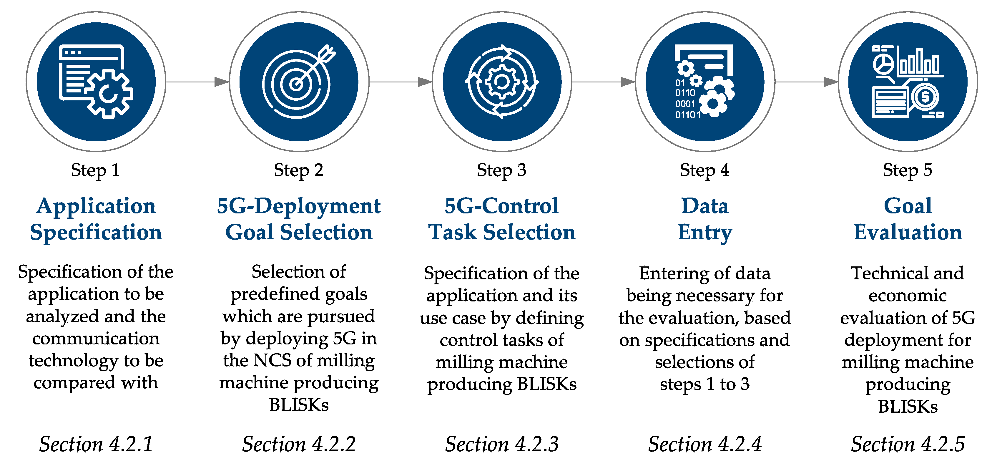
4.2. Application of Approach to Evaluate the Impact of 5G-NSA-NPN on BLISK Milling Process

Consisting of a rotor disk and multiple blades around its edge, the milling of BLISKs is a demanding process. The most common production technology is the milling from solid forged discs, the so-called trochoidal milling [36]. Despite long-lasting research, the BLISK milling process still presents several challenges, especially that of ensuring quality, given there have been failing BLISKs which have led to severe accidents [37].
To ensure the required quality, machine-internal sensors are used to detect critical process parameters, like forces or vibration. However, machine-internal sensors are not always sufficient, leading to milling issues, such as vibration patterns, which affect BLISK quality and require expensive rework. Thus, additional sensors such as acoustic emission (AE) sensors are required for further process improvement. Acoustic emissions are inaudible ultrasonic signals, also known as structural noise. The electrical signals measured in this way consist of characteristic frequencies and sound amplitudes that are specific to the cutting processes. Once a signal is out of the specified and allowed range, the controller of the milling machine reacts to ensure quality. Therefore, the AE sensor can be used for the use case motion control of the milling machine process. Since these sensors must be installed close to the process, wireless communication is a must. For demanding applications such as the monitoring of a 5-axis milling machine, wired sensors are not an option, as they would require a complete new ban planning of the milling process, leading to a decrease in efficiency [38]. To implement the use case, an AE sensor is physically fixed to the BLISK being milled and connected to a 5G-capable UE, also attached to the BLISK, as Figure 9 illustrates according to the defined NCS in Figure 2. The measured frequency is then sent to the cloud-based controller. Here, using among other things, a digital twin- and artificial intelligence (AI)-supported controller, the frequency is constantly compared to the allowed spectrum. Once it is detected that, e.g., a vibration could occur, the actuator adjusts the control variable feed speed v f . This adjustment requires additional production time, however, avoids chattering marks that require rework.
To evaluate the impact of 5G-NSA-NPN on the application, the following sub-sections apply the model of Section 4.1 to the above-described application and use case.

4.2.1. Application Specification

The evaluation of the application bases on the milling of a Ti-6Al-4V BLISK with a 440 mm diameter on a Mikron HMP 800U CNC milling machine from GF Machining Solutions GmbH, which is installed in a test environment at Fraunhofer IPT. In the following, an industrial case scenario is assumed based on the type of BLISK and the milling machine. As described in the introduction of Section 4.2, the use case Motion Control is applied to a Milling Machine. The motion control requires high reliabilities (around 99.999%) and low latencies (between 1 ms to 10 ms). For this reason, no other wireless communication technology can be applied to enable the control tasks [21].
Thus, the 5G scenario is compared to an Ethernet scenario, which does not enable a motion control. As the Mikron milling machine already exists, this case study is a brownfield scenario. For both the Ethernet and the 5G scenario, an identical application is considered.

4.2.2. 5G-Deployment Goal Selection

For the technical analysis, the evaluation model considers seven distinctive goals, which are defined and operationalized in [35]. For the BLISK milling process, three technical goals are relevant. Table 5 summarizes these goals, as well as their key performance indicators (KPI), which are the basis for the further operationalization and quantification of the goals. The goals are defined in such a way that they all have the same optimization direction, i.e., the higher the value of the goal, the better the application. The quantification of the goals is presented in Section 4.2.5.
The economic goals to be considered are the beneficial investment (measured by the net present value (NPV)) and the decrease in operational expenditures ( O P E X ).
Equation (7) defines the N P V as a measure of the beneficial nature of the investment, where i is the annual interest rate, I 0 the initial investment, N the application lifetime, and R t the net cashflow in year t [39].
NPV   ( i , N ) = I 0 t = 1 N   R t ( 1 + i ) t .
Equation (8) defines OPEX per product to calculate operational cost savings, where n t is the amount of produced goods per application in year t.
OPEX Product = OPEX t n t

4.2.3. 5G-Control Task Selection

The control task definition and selection are the core of the evaluation model. First, controlled variables and the main function of the milling machine are mathematically modeled. Second, control tasks for this use case are defined. For a better understanding of the relations between the formula elements, Appendix A provides the important relations. Based on the technical and economic goals, good quantity GQ is the key figure of the mathematical model, more specifically the number of BLISKs passing quality control.
The time to which the good quantity and its depending values refer is one day. GQ is defined in Equation (9), where PQ is the produced quantity SQ the scrap quantity of BLISKs.
GQ = PQSQ
PQ is defined by Equation (10) where AAPT is the actual application production time of the milling machine, PRTP is the planned runtime per BLISK, and t add , BLISK the additional production time in case the motion control adapts the feed speed to avoid chattering marks.
PQ = AAPT PRTP + t add , BLISK
The production of one BLISK on the milling machine is equated to the removal of the necessary material between its blades. PRTP is thus the time it requires to remove this material. It is defined in Equation (11) as the ratio of the total volume of material V BLISK that needs to be milled and the material removal rate MRR milling of the milling machine.
PRTP = V BLISK   MRR milling
To calculate the real milling volume of the BLISK, complex simulations of the BLISK gap would be required, which is the reason why the gap geometry of the BLISK is simplified according to [36,40]. The milling process of the BLISK is separated into three main steps: roughing (1), pre-finishing (2), and finishing (3). Finishing is further separated into blade and hub finishing. Figure 10 shows these configurable processing steps of the milling machine.
The milled volume, as well as the milling process parameters, can be configured for each of these steps, affecting V BLISK , MRR milling and t add , BLISK of each step. As the above-described motion control being enabled by 5G technology controls the feed speed, these milling process steps represent the milling machine’s control tasks in the evaluation model. Table 6 summarizes the control task properties being relevant for the further evaluation of 5G deployment for the milling machine producing BLISK.
As above-mentioned, V BLISK , MRR milling and t add , BLISK differ for each milling step i. Based on the defined control task properties in Table 6, PRTP is defined in Equation (12).
PRTP = i V BLISK , i MRR milling , i = i   ( ( a     d i )   ·   b   · ( h     d i ) )   ·   n blade a p , i   ·   a e , i   ·   v f , i  
V BLISK , i is thereby not affected by the deployment of 5G technology since the required milling volume is given by the BLISK geometry. MRR milling , i is only affected if 5G technology enables a faster feed speed. However, this depends on the material and machine being used, as the feed speed might affect the stability of the process, meaning that a higher feed speed and consequently higher MRR results in vibrations, thus chatter marks on the BLISK surface [41].
In case the AE sensor of the motion control (cf. simplified architecture in Figure 9) detects a vibration occurring, feed speed is reduced to avoid the chatter mark. This leads to an additional processing time t add , BLISK . As this additional time is shorter and cheaper than the manual rework being necessary to remove one mark, the goal is to avoid as many marks as possible. As the feed speed for each of the milling steps is different, t add , i , BLISK differs between the defined processing steps and thus control tasks. Equation (13) defines t add , i , BLISK as a product of the number of vibrations n vibr , react , i per processing step on which the motion control can react on and the additional processing time t add , i resulting from reducing feed speed due to one vibration.
t add , i , BLISK = n vibr , react , i   ·   t add , i
The number of vibrations n vibr , react , i the motion control can react on therefore depends on the network capabilities of 5G. As a prerequisite, a 5G network must fulfill latency requirements. In this case, latency should be a maximum of 10 ms, which is fulfilled by 5G-NSA-NPN (cf. Section 3), even with Release 15. In case this is fulfilled, the influence of network reliability must be considered.
In the model, we assume that n vibr , react , i is the product of network reliability with the total number of vibrations n vibr , i , total . n vibr , i , total is composed of the number of vibrations per minute n vibr , i multiplied by the production time per process step. The latter is in turn calculated by dividing V BLISK , i by MRR milling , i , as shown in Equation (14).
n vibr , react , i = V BLISK , i MRR milling , i   ·   n vibr , i , total   ·   R network
In case motion control is not able to react due to lack of reliability, chatter marks on the BLISK surface occur, requiring manual rework. The number of chatter marks to be reworked n vibr , rework is given in Equation (15).
n vibr , rework = i ( n vibr , mark , i , total     n vibr , react , i   )
Assuming each chatter mark to be reworked causes the same rework time RT BLISK , vibr , total manual rework time caused by chatter marks RT BLISK , vibr , total is given in Equation (16).
RT BLISK , vibr , total = n vibr , rework   ·   RT BLISK , vibr
As rework is executed in parallel to the milling process, RT BLISK , vibr , total has no influence on the planned production time PRTP, hence no effect on PQ. However, it has a major effect on the total work time per product TWT, which is defined in Equation (17).
TWT BLISK = n vibr , rework   ·   RT BLISK , vibr
Now, all influences of 5G technology on the control tasks associated with PQ, AAPT are further considered. AAPT and the associated elements are presented in Equations (18)–(20), where AABT is the actual application busy time, ASUT is the actual application setup time, PABT is the planned application busy time, AADT is the actual application downtime, PADT is the planned application downtime, and UADT is the unplanned application downtime.
AAPT = AABTASUT
AABT = PABTAADT
AADT = PADT + UADT
PADT represents the time per day required for the workpiece and tool change during BLISK production and is defined in Equation (21), where PAOT is the planned application operation time per day, t milling , BLISK is the milling time for one BLISK, t change , workpiece is the changing time of loading and unloading one BLISK, t change , tool is the time required for a tool change, and n change , tool is the number of tool changes per produced BLISK. t milling , BLISK is the sum of the milling times per section and given in Equation (22).
PADT = ( t change , workpiece + t change , tool   ·   n change , tool )   ·   PAOT t milling , BLISK
t milling , BLISK = i t milling , i = i V BLISK , i MRR milling , i
UADT is the unplanned downtime per day emerging from tool damage or breakage of the milling machine and is defined in Equation (23). Tool-related damages and breakages are rated as failure events FE milling , tool . For each failure event, time to repair t FE   milling , tool   breakage is assumed to be identical.
UADT = FE milling , tool     ·   t FE   milling , tool   breakage  
Equation (24) defines FE milling , tool . PAPT is the planned production time of the milling machine. n tooldam is the number of irreparable damages per BLISK per hour, which means irreparable damages to the BLISK caused by tool failures. n toolbreak is the number of tool breakages per hour, i.e., tool damage requiring tool change but not affecting the BLISK quality. PAPT is the difference between the planned application busy time PABT and the application setup time ASUT. However, both n tooldam and n toolbreak are influenced by network reliability. In case tool damage or breakage is detected in time via motion control, the tool is changed or stopped and would not cause any failure. However, if the network is not available or reliable, the tool causes failure. As the occurrence of tool failures over time is also dependent on the BLISK process step, n tooldam and n toolbreak are the weighted sum of tool damages over the milling time, as Equations (25) and (26) show.
FE milling , tool = PAPT   ·   ( n tooldam + n toolbreak ) = ( PABT     ASUT )   ·   ( n tooldam + n toolbreak )
n tooldam   = i n tooldam , i   ·   t milling , i t milling , BLISK   ·   ( 1 R network )
n toolbreak   = i n toolbreak , i   ·   t milling , i t milling , BLISK   ·   ( 1     R network )  
With this, mathematical relations to calculate PQ are derived. To now determine all relevant mathematical relations between control tasks and the key figure good quantity GQ (cf. Equation (9)), scrap quantity SQ is further considered. Scrap emerges due to the above-mentioned tool damage. Assuming that at maximum, one critical tool damage occurs per BLISK, critical tool damage is synonymous with a scrap BLISK, as shown in Equation (27).
SQ BLISK = n tooldam   ·   PAPT milling  
Thus, all relevant mathematical relations to calculate the key figure GQ are derived.
Table 7 summarizes the control task configurations being necessary for the second case study according to the definitions in Table 6. For the control tasks, BLISK geometry is given by [42]. The data for roughing, pre-finishing, and finishing is given by [43]. Based on industrial expert knowledge, it is assumed that the feed speed can be slightly increased in the 5G-deployed process, as more precise motion control is enabled. Furthermore, as feed speed adoption is enabled by 5G technology, it is only relevant for the 5G-deployed scenario.

4.2.4. Data Entry

Based on the chosen goals, necessary data are defined by the evaluation model. Thereby, data are distinguished into five categories, which are application data, product data, process data, failure data, and facility data then further categorized between technical data and economic data to facilitate the data entry. By connecting the evaluation data with the chosen goals, the user does not enter “unnecessary” data but only relevant data.
Table A1 in Appendix B shows the use case data and allocates them to the chosen goals in Section 4.2.2. It further shows where the data originates. U hereby stands for “User”, and L stands for “Literature”. The users are thereby expert teams consisting of representatives of the research project 5G-SMART.

4.2.5. Goal Evaluation

Finally, to evaluate the goals and thus the benefits of 5G technology deployment, the delta between the 5G-value and the value of the communication technology to be compared is calculated.
The technical goals are calculated by averaging the delta of the KPIs. Since the goals are all defined with a positive optimization direction (the higher, the better), the delta of KPIs with a positive trend is added whereas the delta of KPIs with a negative trend is subtracted. Equation (28) shows an example for the goal “Quality”. The other goals are calculated based on the same scheme.
Δ Quality = ( FPY 5 G     FPY Ethernet ) + ( QR 5 G     QR Ethernet )     ( RR 5 G     RR Ethernet )     ( SR 5 G     SR Ethernet ) 4
For the economic goals, Equation (29) shows the calculation exemplary for the NPV.
Δ NPV = NPV 5 G     NPV Ethernet  
Based on the influence of the control tasks shown in Section 4.2.3, the data derived in Section 4.2.4 and according to the formula presented above, technical, and economic goals are analyzed. The reliability of 99.9953% is used for the evaluation, as this was the lowest measured reliability of 5G-NSA-NPN. Figure 11 presents the delta of technical goals of 5G technology compared to the original use case with no motion control. The goals are thereby evaluated based on the reference frame of one year. As portrayed in Figure 11a, all goals have a positive delta, meaning 5G leads to an improvement. Figure 11b shows the delta of the corresponding KPIs as well as their optimization trend. As for the overall goals, the majority of KPIs show an improvement.
Figure 12 shows the difference between the NPV of a 5G-controlled BLISK milling process with motion control, compared to one with no motion control. Thereby, 5G-NSA-NPN was assumed. This means, the network is owned by the manufacturer and no service costs are incurred by the mobile network operator. Furthermore, as investment costs for 5G hardware are currently still uncertain, they were not considered in the delta shown. The cash flow is assumed constant over the 10 years. This means that the delta NPV is the maximum value the company can invest into 5G hardware, 5G deployment costs, additional operational costs, and machining hardware to stay beneficial, which is around EUR 2.6 m for 10 years. The massive decrease in manual rework has a positive impact on the NPV. This becomes even more clear when considering the OPEX per product.
Equation (30) shows the difference in OPEX per product. Here, it becomes clear that the operational costs per product are reduced, while more BLISKs are produced. This leads to a reduction of over EUR 1000 per BLISK.
Δ OPEX Product = OPEX 5 G PQ 5 G     OPEX Ethernet PQ Ethernet   = 6,648,995 258     6,570,945 251   = 1036  
Thus, both, the technical and economic evaluation shows a positive effect when deploying 5G-NSA-NPN in an NCS of the BLISK milling process.

5. Conclusions and Outlook

The paper analyzed the technical and economic effects of 5G-NSA-NPN for closed-loop control in production, with an exemplar shown for a BLISK milling use case. First, the network performance of 5G-NSA-NPN at Fraunhofer IPT was evaluated, showing suitability for the BLISK milling process. Second, the evaluation model developed in [33] set the basis for the techno-economic analysis of 5G-NSA-NPN for the BLISK milling process. The analysis showed the positive effects of 5G compared to an Ethernet-based control without motion control use case for both technical, as well as, economic goals. The case analysis confirmed the positive influence. However, the analysis did not include any capital expenditures or additional operational expenditures of 5G infrastructure and thus shows, in terms of the economic analysis, how much money companies could invest in 5G. Once reliable data for 5G capital expenditures and operational expenditures, as well as for 5G UE are available, the analysis might be improved.
For further research, two points are highlighted: on the one hand, from a network performance point of view, the performance characteristics of stand-alone networks shall be evaluated, to analyze whether the network characteristics can even be improved. On the other hand, this approach is an ex-ante approach, thus the evaluation is theoretical and not validated with a long-term test of the BLISK milling process. This validation should be conducted to prove the theoretical values presented in this paper. However, as the milling of a BLISK takes several days and the product itself is very expensive, these tests must be well-planned and should be conducted on a blade level.

Author Contributions

Conceptualization, R.K. and S.S.; formal analysis, R.K. and S.S.; methodology, R.K., K.S. and A.M. writing—original draft preparation, R.K. and S.S.; writing—review and editing, M.B., N.K., T.V. and R.H.S.; visualization, R.K.; supervision, N.K., T.V. and R.H.S.; project administration, N.K.; funding acquisition, N.K. All authors have read and agreed to the published version of the manuscript.

Funding

This work has been performed in the framework of the H2020 project “5G-SMART” co-funded by the EU and the project “5G-Industry Campus Europe”, which is funded by the BMVI with the funding code VB5GICEIPT. The authors would like to acknowledge the contributions of their colleagues. This information reflects the consortium’s view, but the consortium is not liable for any use that may be made of the information contained therein.

Conflicts of Interest

The authors declare no conflict of interest.

Appendix A. Mathematical Model Explanations

Figure A1. Core elements of mathematical model and their relation.
Electronics 11 01736 g0a1

Appendix B. Use Case Data

Table A1. List of formula symbols.
DataUnitValueData TypeData SourceGoal
ProductivityQualitySustainabilityNPV and RoI
Application—Total Number[ ]1ApplicationU x
Application—Lifetimey10ApplicationU x
Tool Change—Durationh0.166ApplicationUxxxx
Tool Change—Number of Change per BLISK[ ]1ApplicationUxxxx
Workpiece Change—Durationh0.166FacilityUxxxx
Compressed Air—Consumption of ApplicationL/min150FacilityU xx
Compressed Air—Consumption of ReworkL/min260FacilityU xx
Compressed Air—Cost€/L0.01FacilityU x
Convergence Factor from kWh to CO2kg CO2/kWh3FacilityL xx
Electric Power—Cost€/kWh0.319FacilityU x
Electric Power—Hourly Appl. ConsumptionkW13FacilityU xx
Electric Power—Hourly Network ConsumptionkW1FacilityL xx
Electric Power—Hourly Rework ConsumptionkW1FacilityU xx
Energy—CO2 Tax€/t30FacilityU x
Gas—ConsumptionBTU0FacilityU xx
Water—Consumption l/h50FacilityU xx
Water—Cost€/L0.05FacilityU x
Failure Events—Accidents per Day[ ]0FailureU x
Failure Events—Costs for Tool Breakage1000FailureU x
Failure Events—TTR per Tool Breakageh2FailureUxxxx
Failure Events—Wage of Repairment Staff€/h35FailureU x
Application Downtime—Planned—Cost€/h180ProcessU x
Application Downtime—Unplanned—Cost€/h1500ProcessU x
Application Maintenance—Time per Operationh2ProcessUxxxx
Application Maintenance—Operations per Day[ ]0.2ProcessUxxxx
Application Operation Time—Planned per Dayh16ProcessUxxxx
Application Setup—Number per Day[ ]1ProcessUxxxx
Application Setup—Time per Setuph0.5ProcessUxxxx
Application Setup—Wage of Setup Staff€/h35ProcessU x
Batch Size[ ]1ProcessUxxxx
Human Operation—Operator per Shift[ ]1ProcessU x
Human Operation—Planned Break Time/Shifth0.5ProcessUx x
Human Operation—Planned Work Time/Shift h8ProcessUx x
Human Operation—Shifts per Day[ ]2ProcessUx x
Human Operation—Wage of Staff€/h35ProcessU x
Production—Days per Yeard250ProcessUxxxx
Disposal—Cost per Part5000ProductU x
Individualization—Additional Profit0ProductU x
Individualization—Percentage%0ProductU x
Material—Cost per Part1500ProductU x
Material—Cost for Rework per Part0ProductU x
Products—Selling Price per Part27,500ProductU x
Quality Control—Inspection Percentage%100ProductU xxx
Quality Control—Inspection Time per Parth4ProductU x x
Quality Control—Cost per Part1000ProductU x
Rework—Duration—Basic for one Parth4ProductU xxx
Rework—Duration—Per Vibrations60ProductU xxx
Rework—Wage of Staff€/h35ProductU x
Rework—Percentage%100ProductU x x
Annual Interest Rate%5AdditionalU x

References

  1. Aijaz, A.; Stanoev, A. Closing the Loop: A High-Performance Connectivity Solution for Realizing Wireless Closed-Loop Control in Industrial IoT Applications. IEEE Internet Things J. 2021, 8, 11860–11876. [Google Scholar] [CrossRef]
  2. Jeschke, S.; Brecher, C.; Meisen, T.; Özdemir, D.; Eschert, T. Industrial Internet of Things and Cyber Manufacturing Systems. In Industrial Internet of Things; Springer: Berlin/Heidelberg, Germany, 2017; pp. 3–19. [Google Scholar]
  3. Lyczkowski, E.; Wanjek, A.; Sauer, C.; Kiess, W. Wireless Communication in Industrial Applications. In Proceedings of the 2019 24th IEEE International Conference on Emerging Technologies and Factory Automation (ETFA), Zaragoza, Spain, 10–13 September 2019; pp. 1392–1395. [Google Scholar]
  4. Åkerberg, J.; Gidlund, M.; Björkman, M. Future Research Challenges in Wireless Sensor and Actuator Networks Targeting Industrial Automation. In Proceedings of the 2011 9th IEEE International Conference on Industrial Informatics, Lisbon, Portugal, 26–29 July 2011; pp. 410–415. [Google Scholar]
  5. Baumann, D.; Mager, F.; Wetzker, U.; Thiele, L.; Zimmerling, M.; Trimpe, S. Wireless Control for Smart Manufacturing: Recent Approaches and Open Challenges. Proc. IEEE 2020, 109, 441–467. [Google Scholar] [CrossRef]
  6. Siegl, S. Networked Control Systems: Ein Überblick; Universität der Bundeswehr München: Munich, Germany, 2017. [Google Scholar]
  7. Zuehlke, D. SmartFactory—Towards a Factory-of-Things. Annu. Rev. Control 2010, 34, 129–138. [Google Scholar] [CrossRef]
  8. Scheuvens, L.; Simsek, M.; Noll-Barreto, A.; Franchi, N.; Fettweis, G.P. Framework for Adaptive Controller Design Over Wireless Delay-Prone Communication Channels. IEEE Access 2019, 7, 49726–49737. [Google Scholar] [CrossRef]
  9. Schulz, P.; Matthe, M.; Klessig, H.; Simsek, M.; Fettweis, G.; Ansari, J.; Ashraf, S.A.; Almeroth, B.; Voigt, J.; Riedel, I. Latency Critical IoT Applications in 5G: Perspective on the Design of Radio Interface and Network Architecture. IEEE Commun. Mag. 2017, 55, 70–78. [Google Scholar] [CrossRef]
  10. Varghese, A.; Tandur, D. Wireless Requirements and Challenges in Industry 4.0. In Proceedings of the 2014 International Conference on Contemporary Computing and Informatics (IC3I), Mysore, India, 27–29 November 2014; pp. 634–638. [Google Scholar]
  11. Stefanović, Č. Industry 4.0 from 5G Perspective: Use-Cases, Requirements, Challenges and Approaches. In Proceedings of the 2018 11th CMI International Conference: Prospects and Challenges towards Developing a Digital Economy within the EU, Copenhagen, Denmark, 29–30 November 2018; pp. 44–48. [Google Scholar]
  12. Aijaz, A. Private 5G: The Future of Industrial Wireless. arXiv 2020, arXiv:2006.01820. [Google Scholar] [CrossRef]
  13. Adib, D.; Barraclough, C. 5G’s Impact on Manufacturing-$740 BN of Benefits in 2030. STL Partn. Exec. Brief 2019, 1, 1–40. [Google Scholar]
  14. Boston Consulting Group. 5G Promises Massive Job and GDP Growth in the US. 2021. Available online: https://www.bcg.com/publications/2021/5g-economic-impact-united-states (accessed on 27 April 2022).
  15. MHP Management und IT-Beratung. Industrie 4.0 Barometer 2020; MHP Management und IT-Beratung: Munich, Germany, 2021. [Google Scholar]
  16. Digital Catapult. Made in 5G—5G for the UK Manufacturing Sector; UK5G: London, UK, 2019. [Google Scholar]
  17. 5G Alliance for Connected Industries and Automation. 5G Non-Public Networks for Industrial Scenarios; ZVEI–German Electrical and Electronic Manufacturers’ Association: Frankfurt am Main, Germany, 2019. [Google Scholar]
  18. Gupta, R.A.; Chow, M.-Y. Networked Control System: Overview and Research Trends. IEEE Trans. Ind. Electron. 2010, 57, 2527–2535. [Google Scholar] [CrossRef]
  19. Xia, F.; Tian, Y.-C.; Li, Y.; Sung, Y. Wireless Sensor/Actuator Network Design for Mobile Control Applications. Sensors 2007, 7, 2157–2173. [Google Scholar] [CrossRef] [PubMed]
  20. Chow, M.-Y.; Tipsuwan, Y. Network-Based Control Systems: A Tutorial. In Proceedings of the IECON’01. 27th Annual Conference of the IEEE Industrial Electronics Society (Cat. No. 37243), Denver, CO, USA, 29 November–2 December 2001; pp. 1593–1602. [Google Scholar]
  21. Kiesel, R.; Jakob, F.; Vollmer, T.; Schmitt, R.H. Evaluation of ICT for Networked Control Systems of Latency-Critical Applications in Production. In Proceedings of the 15th CIRP Conference on Intelligent Computation in Manufacturing Engineering, Gulf of Naples, Italy, 13–15 July 2022. (currently being published). [Google Scholar]
  22. Ploplys, N.J.; Kawka, P.A.; Alleyne, A.G. Closed-Loop Control over Wireless Networks. IEEE Control Syst. Mag. 2004, 24, 58–71. [Google Scholar]
  23. Kartashevskiy, V.; Buranova, M. Analysis of packet jitter in multiservice network. In Proceedings of the 2018 International Scientific-Practical Conference Problems of Infocommunications. Science and Technology (PIC S&T), Kharkiv, Ukraine, 9–12 October 2018; pp. 797–802. [Google Scholar]
  24. Leng, Q.; Wei, Y.-H.; Han, S.; Mok, A.K.; Zhang, W.; Tomizuka, M. Improving control performance by minimizing jitter in RT-WiFi networks. In Proceedings of the 2014 IEEE Real-Time Systems Symposium, Rome, Italy, 2–5 December 2014; pp. 63–73. [Google Scholar]
  25. She, C.; Yang, C.; Quek, T.Q. Radio resource management for ultra-reliable and low-latency communications. IEEE Commun. Mag. 2017, 55, 72–78. [Google Scholar] [CrossRef]
  26. Dahlman, E.; Parkvall, S.; Skold, J. 5G NR: The Next Generation Wireless Access Technology; Academic Press: Cambridge, MA, USA, 2020. [Google Scholar]
  27. Ericsson. 5G Deployment Considerations; Ericsson: Stockholm, Sweden, 2018; Available online: https://www.ericsson.com/en/reports-and-papers/5g-deployment-considerations (accessed on 27 April 2022).
  28. Siddiqi, M.A.; Yu, H.; Joung, J. 5G Ultra-Reliable Low-Latency Communication Implementation Challenges and Operational Issues with IoT Devices. Electronics 2019, 8, 981–998. [Google Scholar] [CrossRef] [Green Version]
  29. NGMN Alliance. 5G E2E Technology to Support Verticals URLLC Requirements. 2019. Available online: https://www.ngmn.org/wp-content/uploads/200210-Verticals-URLLC-Requirements-v2.5.4.pdf (accessed on 27 April 2022).
  30. International Telecommunication Union. Recommendation ITU-R M.2083-0: IMT Vision—Framework and Overall Objectives of the Future Development of IMT for 2020 and Beyond; International Telecommunication Union: Geneva, Switzerland, 2015. [Google Scholar]
  31. Ghosh, A.; Maeder, A.; Baker, M.; Chandramouli, D. 5G Evolution: A View on 5G Cellular Technology beyond 3GPP Release 15. IEEE Access 2019, 7, 127639–127651. [Google Scholar] [CrossRef]
  32. Lennvall, T.; Gidlund, M.; Åkerberg, J. Challenges when Bringing IoT into Industrial Automation. In Proceedings of the 2017 IEEE AFRICON, Cape Town, South Africa, 18–20 September 2017; pp. 905–910. [Google Scholar]
  33. Kiesel, R.; Böhm, F.; Pennekamp, J.; Schmitt, R.H. Development of a Model to Evaluate the Potential of 5G Technology for Latency-Critical Applications in Production. In Proceedings of the IEEE International Conference on Industrial Engineering and Engineering Management (IEEM) 2021, Singapore, 13–16 December 2021; pp. 739–744. [Google Scholar]
  34. Kiesel, R.; Henke, L.; Mann, A.; Renneberg, F.; Stich, V.; Schmitt, R.H. Techno-Economic Evaluation of 5G Technology for Automated Guided Vehicles in Production. Electronics 2022, 11, 192. [Google Scholar] [CrossRef]
  35. Kiesel, R.; Stichling, K.; Hemmers, P.; Vollmer, T.; Schmitt, R.H. Quantification of Influence of 5G Technology Implementation on Process Performance in Production. In Proceedings of the 54th CIRP Conference on Manufacturing Systems, Athen, Greece, 22–24 September 2021; pp. 104–109. [Google Scholar]
  36. Klocke, F.; Zeis, M.; Klink, A.; Veselovac, D. Technological and Economical Comparison of Roughing Strategies via Milling, EDM and ECM for Titanium-and Nickel-Based BLISKs. Procedia Cirp 2012, 2, 98–101. [Google Scholar] [CrossRef]
  37. Ericsson. 5G Business Value—A Case Study on Real-Time Control in Manufacturing; Ericsson: Stockholm, Sweden, 2018; Available online: https://www.ericsson.com/en/reports-and-papers/consumerlab/reports/5g-business-value-to-industry-blisk (accessed on 27 April 2022).
  38. Kehl, P.; Lange, D.; Maurer, F.K.; Németh, G.; Overbeck, D.; Jung, S.; König, N.; Schmitt, R.H. Comparison of 5G Enabled Control Loops for Production. In Proceedings of the 2020 IEEE 31st Annual International Symposium on Personal, Indoor and Mobile Radio Communications, London, UK, 31 August–3 September 2020; pp. 1–6. [Google Scholar]
  39. Pike, R.; Neale, B.; Linsley, P. Corporate Finance and Investment: Decisions & Strategies; Pearson Education Limited: Harlow, UK, 2015. [Google Scholar]
  40. Klocke, F.; Zeis, M.; Klink, A.; Veselovac, D. Technological and Economical Comparison of Roughing Strategies via Milling, Sinking-EDM, Wire-EDM and ECM for Titanium- and Nickel-Based Blisks. CIRP J. Manuf. Sci. Technol. 2013, 6, 198–203. [Google Scholar] [CrossRef]
  41. Klocke, F. Fertigungsmesstechnik und Werkstückqualität. In Fertigungsverfahren 1; Springer: Berlin/Heidelberg, Germany, 2018; pp. 5–45. [Google Scholar]
  42. Fricke, K.; Gierlings, S.; Ganser, P.; Venek, T.; Bergs, T. Geometry Model and Approach for Future Blisk LCA. In Proceedings of the IOP Conference Series: Materials Science and Engineering, Chennai, India, 16–17 September 2020. [Google Scholar] [CrossRef]
  43. Calleja, A.; González, H.; Polvorosa, R.; Gómez, G.; Ayesta, I.; Barton, M.; de Lacalle, L.L. Blisk Blades Manufacturing Technologies Analysis. Procedia Manuf. 2019, 41, 714–722. [Google Scholar] [CrossRef]
Figure 1. Structure of the paper.
Electronics 11 01736 g001
Figure 2. Architecture of the networked control system being referred to in this paper [21].
Electronics 11 01736 g002
Figure 3. Latencies in a networked control system.
Electronics 11 01736 g003
Figure 4. Experimental setup for 5G performance measurements with ping and Hawkeye test.
Electronics 11 01736 g004
Figure 5. Latency measurements with ping and Hawkeye tests for D2D communication in 5G-NSA.
Electronics 11 01736 g005
Figure 6. Jitter measurements with ping and Hawkeye tests for D2D communication in 5G-NSA.
Electronics 11 01736 g006
Figure 7. Comparison of expected (orange) vs. measured D2D reliability in 5G-NSA.
Electronics 11 01736 g007
Figure 8. Section structure and evaluation approach for techno-economic evaluation of 5G technology for milling machine producing BLISKs according to [33].
Electronics 11 01736 g008
Figure 9. Simplified illustration of a milling machine producing BLISKs controlled via 5G-deployed NCS and corresponding control data flow.
Electronics 11 01736 g009
Figure 10. Configurable processing steps of milling machine producing BLISKs representing its control tasks.
Electronics 11 01736 g010
Figure 11. Influence of 5G technology and motion control use case compared to Ethernet and no motion control use case on technical goals. (a) all goals with a positive delta; (b) the delta of the corresponding KPIs as well as their optimization trend.
Electronics 11 01736 g011aElectronics 11 01736 g011b
Figure 12. Influence of 5G technology and motion control use case compared to Ethernet and no motion control use case for NPV.
Electronics 11 01736 g012
Table 1. Overview of 5G frequency ranges and bands [26,27].
Frequency Range DesignationFrequency Band Existing/NewFrequency Range [MHz]
FR1Low BandsExisting/New410–960
Mid Bands IExisting1000–2600
Mid Bands IINew3300–7125
FR2High BandsNew24,250–52,600
Table 2. Latency and jitter results from ping and Hawkeye test in 5G-NSA.
Ping TestHawkeye [from → to]Hawkeye [to → from]
Latency [ms]Jitter [ms]Latency [ms]Jitter [ms]Latency [ms]Jitter [ms]
Nr.Avg.Min.Max.Avg.Avg.Min.Max.Avg.Avg.Min.Max.Avg.
111.107.6618.701.8811.61716111.697161.23
210.957.4717.321.8111.737171.0211.738151.15
311.017.7616.681.8411.758160.9811.717161.14
411.157.0920.432.0712.058161.3812.118181.07
511.167.3617.312.0411.806151.3712.187171.09
610.977.2717.201.8711.758161.3111.958181.06
711.087.5219,211.9112.037151.3311.748191.11
811.177.4619.912.0412.097161.3612.338161.09
911.227.4117.802.0212.147171.4711.798171.08
1011.067.4318.191.9612.065171.5711.678161.08
Table 3. Iperf3 results for UDP packages in a 5G-NSA network.
Nr.Loss [%]Reliability [%]
10.002799.9973
20.001399.9987
30.002799.9973
40.004099.9960
50.002799.9973
60.002799.9973
70.001399.9987
80.004799.9953
90.001399.9987
100.004099.9960
Table 4. Summary of measured 5G-NSA-NPN values and comparison to nominal values.
Performance CharacteristicTest MethodNominal Value According to ITU SpecificationsMeasured Mean-Value at IPT NSA-NPN
Jitter [ms]Hawkeye/Pingn/a1.19/1.94
Latency [ms]Hawkeye/Ping1.011.89/11.09
Loss [%]iperf30.0010.003
Reliability [%]Iperf399.99999.997
Table 5. Technical goals when implementing 5G technology for BLISK milling process.
GoalDescriptionKey Performance IndicatorTrend
ProductivityOutput per unit of input over a specific period; also: production efficiencyEffectiveness (E)Max
Throughput Ratio (TR)Max
Worker Efficiency (WE)Max
QualityDegree to which the output of the production process meets the requirementsFirst Pass Yield (FPY)Max
Quality Ratio (QR)Max
Rework Ratio (RR)Min
Scrap Ratio (SR)Min
SustainabilityLevel to which the creation of manufactured products is fulfilled by processes that are nonpollutingCompressed Air Consumption Ratio (ACR)Min
Electric Power Consumption Ratio (ECR)Min
Gas Consumption Ratio (GCR)Min
Water Consumption Ratio (WCR)Min
Table 6. BLISK processing control task properties being relevant for the evaluation of 5G deployment and their formula symbols.
Control Task PropertyUnitRoughing
i = r
Pre-Finishing
i = p
Finishing (Blade)
i = f,b
Finishing (Hub)
i = f,h
Cutting Depth (Axial)mm a p , r a p , p a p , f a p , f
Cutting Depth (Radial)mm a e , r a e , p a e , f a e , f
Feed Speedmm/s v f , r v f , p v f , f , b v f , f , h
Feed Speed Adoption Times t add , r t add , p t add , f , b t add , f , h
Surface Thicknessmm d r d p d f , b d f , h
Tool Breakagen°/h n toolbreak , r n toolbreak , p n toolbreak , f , b n toolbreak , f , h
Tool Damagen°/h n tooldam , r n tooldam , p n tooldam , f , b n tooldam , f , h
Vibrations causing Marksn°/min n vibr , r n vibr , p n vibr , f , b n vibr , f , h
Table 7. Case study values for control tasks of milling machine producing BLISKs.
Control Task PropertyUnitRoughing
i = r
Pre-Finishing
i = p
Finishing (Blade)
i = f,b
Finishing (Hub)
i = f,h
Cutting Depth (Axial)mm7.55.00.60.6
Cutting Depth (Radial)mm2.02.00.51.0
Feed Speed (without 5G)mm/min1200730350450
Feed Speed (with 5G)mm/min1250750360460
Feed Speed Adoption Times0.000.255.001.00
Surface Thicknessmm10.05.00.0110.017
Tool Breakagen°/h1/10,0001/10,0001/100,0001/100,000
Tool Damagen°/h1/100,0001/100,0001/100,0001/100,000
Vibrations causing Marksn°/min0.000.010.200.10
Publisher’s Note: MDPI stays neutral with regard to jurisdictional claims in published maps and institutional affiliations.

