Efficient Perineural Invasion Detection of Histopathological Images Using U-Net

Abstract

Perineural invasion (PNI), a sign of poor diagnosis and tumor metastasis, is common in a variety of malignant tumors. The infiltrating patterns and morphologies of tumors vary by organ and histological diversity, making PNI detection difficult in biopsy, which must be performed manually by pathologists. As the diameters of PNI nerves are measured on a millimeter scale, the PNI region is extremely small compared to the whole pathological image. In this study, an efficient deep learning-based method is proposed for detecting PNI regions in multiple types of cancers using only PNI annotations without detailed segmentation maps for each nerve and tumor cells obtained by pathologists. The key idea of the proposed method is to train the adopted deep learning model, U-Net, to capture the boundary regions where two features coexist. A boundary dilation method and a loss combination technique are proposed to improve the detection performance of PNI without requiring full segmentation maps. Experiments were conducted with various combinations of boundary dilation widths and loss functions. It is confirmed that the proposed method effectively improves PNI detection performance from 0.188 to 0.275. Additional experiments were also performed on normal nerve detection to validate the applicability of the proposed method to the general boundary detection tasks. The experimental results demonstrate that the proposed method is also effective for general tasks, and it improved nerve detection performance from 0.511 to 0.693.

1. Introduction

Perineural invasion (PNI), an important pathological feature of many malignancies, is the attachment of tumor cells to nerves [1,2,3]. In many cancers, the detection of PNI indicates a high risk of local recurrence and reduced survival [4,5]. The diagnostic criterion for the pathological diagnosis of PNI is cancer surrounding at least 33% of the nerve, which is detected by pathologists in microscopic examinations of tissue specimens [6,7]. The detection of PNI in small nerves on glass slides is a labor-intensive task [8]. Moreover, because tumor cells exhibit different morphologies depending on histological types and organs, and the infiltrating patterns of tumor cells are highly variable, it is difficult to model cancer in all organs [9,10].

Deep learning approaches have recently shown remarkable performance in various medical imaging applications [11,12]. Previous studies applied deep learning methods to histopathological images (whole slide images, WSIs). A detect-then-segment framework [13] was proposed inspired by the Mask-R-convolutional neural network (CNN) [14] for glomerular segmentation. A new framework for colonoscopy tissue segmentation and classification was also proposed along with a two-stage pipeline with multi-instance approach for gastric image segmentation [15]. Other advances include the design of a deep CNN to detect clinical heart failure [16], a transfer-learning-based framework [17], and a weakly supervised learning method for lung cancer classification [18]. Because of the high dimensionality of WSI, almost all previous studies utilizing deep learning on WSI have extracted patches for benign and malignant lesions to train deep learning models. However, to extract patches from a WSI, malignant and benign labels are required. This annotation is usually performed by pathologists, which is labor-intensive and time-consuming, and it is almost impossible to accurately annotate pixel-by-pixel. As a form of PNI is when tumor cells invade or touch nerves, annotations for all tumor and nerve cells are required for PNI detection.

In this study, an efficient approach is proposed for PNI detection in multiple organ cancers of WSI using U-Net [19], a deep learning model for image segmentation. The proposed method does not require tumor and nerve information and efficiently detects PNI with only a small amount of PNI annotation. The deep learning model is trained to model the patterns around the boundary between two different regions using patches containing both tumor and nerve cells. To exploit the information near the PNI, a boundary dilation method is proposed to expand the boundary area between the tumor and nerve cells. Experiments were conducted with various combinations of boundary dilation widths and loss functions to prove that our proposed method should effectively improve the PNI detection performance. Experiments were also conducted in an additional study on nerve detection, and the results show that our method can be utilized for general boundary detection tasks. The contributions of this study are summarized as follows:

✓

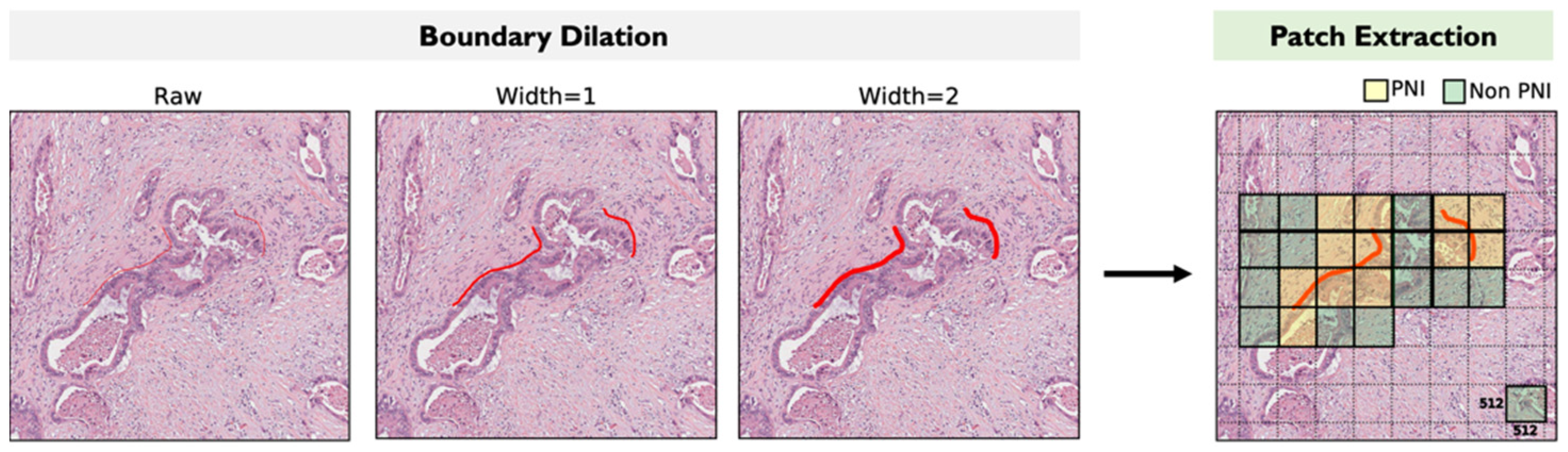
A deep learning-based method is proposed to efficiently detect PNI region with a relatively small amount of data with various types of cancers. The proposed method can learn a neural network model without detailed labels for the nerve and tumor cells. Labeling cells requires intensive and time-consuming labor from well-trained physicians. Instead, only the boundary lines between those cells are used to learn the models.

✓

A boundary dilation method and a loss combination technique are proposed to improve the detection performance of PNI. The expanded regions by the proposed dilation method help model the visual transitional patterns from the nerve to the tumor cells. A new loss function is also proposed to better learn the neural network model. Experimental results confirm that the proposed method effectively improves PNI detection performance from 0.188 to 0.275.

✓

We validate that the proposed method can be utilized in many other medical problems that are involved with boundary detection tasks. According to the experimental results for nontumor and nerve cells boundary detection, the proposed method is effective for general boundary detection, and it showed improved detection performance from 0.551 to 0.693.

2. Related Work

The detection of PNI in multiple cancer types was originally proposed by the pathology AI platform (PAIP) 2021 challenge [20]. In this challenge, top 10 teams according to the attained detection performances are selected, and their methods and results are presented in the challenge website. The target tasks of the challenge are PNI classification and PNI region segmentation, and most top 10 ranked methods adopt two-stage approaches: classification followed by segmentation. Patches containing PNI junctions are first extracted by a classifier, and then the input image is partitioned into cancer and nerve cell regions using a segmentation model. An alternate method is finding tumor and nerve areas independently to identify their boundary as PNI. One of the top 10 teams proposed a feature pyramid network (FPN) for PNI segmentation [21]. The multiscale feature maps from FPN layers were aggregated to obtain more precise segmentation masks [21]. Another method is applying PNI classification, tumor and nerve segmentation, and PNI detection using hand-crafted features and a random forest classifier [22]. Because the PAIP challenge does not provide the final evaluation set to rank the submitted codes, most of the methods reported their performance with the released training data only. Therefore, the performances reported in those papers are different from the performance indices shown on the challenge website. Both of the previous methods utilized all of the annotation information such as nerve regions, tumor cell regions, nontumor cells, and the PNI boundary lines. However, annotating all of these kinds of information on the raw whole-slide images requires intensive labor from well-trained pathologists. Hence, complete training data are not always available. The proposed method is aimed at developing a method requiring only PNI junction lines. Instead of using full annotation, the boundary areas are expanded to model the transitional changes between nerve and tumor cells. The proposed model successfully detects the PNI junctions.

3. Methods

We propose a deep learning-based method to efficiently detect PNI junctions using PNI annotations only. A boundary dilation method and a loss combination technique are proposed to improve the detection performance. As mentioned in Section 2, it is hard to make a fair comparison because the input features and target information are different. However, the proposed method is applicable to many other problems without sophisticated, hand-drawn segmentation maps for the targets. The proposed method is also applicable to non-PNI problems, such as normal nerve detection.

3.1. Proposed Boundary Dilation Method

The characteristic histopathological observation of PNI involves the nerve cells infiltrated or enclosed by tumor cells. The detection of PNI requires information on the nerve cells, the tumor cells surrounding the nerve, and PNI. The annotation is a manual, labor-intensive task that must be performed by pathologists. The proposed method does not require tumor and nerve annotations for PNI detection. Only PNI junction annotation is used to detect PNI. Therefore, less annotation labor is required, and the detection performance is less affected by human errors. Nerve and tumor cells inevitably coexist around the PNI. The main purpose of the proposed method is to automatically learn the boundary patterns between the nerve and tumor cell regions, instead of the exact locations of those cells. In other words, the model learns to capture the boundary between the nerves and tumors using input patches that contain both types of cells. Raw annotations for PNI are usually provided by one-pixel width lines that are hardly visible in the raw high-resolution WSI. In Figure 1, the red box in the leftmost image is magnified, and the blue boxes in the second left image are magnified again to clearly visualize the PNI. As shown in Figure 1, the number of PNI pixels is too small compared to that of the whole image. Moreover, the hand-labeled ground-truth PNI lines are often inaccurate because they can be biased by individual pathologists. To overcome these limitations, a boundary dilation method that expands the boundary between two different regions is proposed to exploit the information near PNI and compensate for human error in PNI annotation.

The proposed boundary dilation method is conceptually illustrated in Figure 2. The raw one-pixel boundary line expands to the left and right by a variable width factor. For example, if the width is set to 1, the one-pixel raw boundary will expand by 1 pixel in both the left and the right directions. Similarly, if the dilation width is set to 2, the one-pixel raw boundary will expand two pixels to the left and two pixels to the right, on the basis of the raw boundary pixel. We then split the whole WSI image into smaller patches for efficient model training. Around the dilated PNI annotations, a sliding window scheme with 50% overlap is used to extract patches for PNI and non-PNI of size (512 × 512). Consequently, there are two classes of extracted patches: PNI containing both nerves and tumors, and the remaining non-PNI.

Figure 3 compares two different dilation widths for the same PNI annotations with the widths set to 1 (top row) and 2 (bottom row). The green lines represent PNI annotations with expansions to the left and right. As mentioned in Section 1, each PNI is characterized by different morphology, scale, and infiltrating patterns. In some cases, a nerve is completely surrounded by tumor cells, whereas, in other cases, tumor cells partially touch the nerve. From the data provided for challenge, it can be shown that the raw PNI annotations are usually generated with bias toward tumor cells. By expanding the PNI boundary, more information becomes available on the area near the PNI, thus avoiding the inaccuracies incurred by human error or biases.

3.2. End-to-End PNI Detection and Segmentation with Combined Loss

The segmentation model can be trained with only segmentation loss. In this task, the segmentation loss that is calculated from true PNI mask and predicted PNI mask used to train the PNI segmentation model. We use only the PNI boundary labels of the training data. The model trained with such a small area of the dataset may not be robust for other, non-boundary areas. The existence of the PNI boundary in a patch is determined by the value of 2D global max pooling. We propose combined loss for the segmentation and classification targets. The combined loss functions can be expressed as follows:

$$L_{seg}=D\left(M\left(x\right),y\right), L_{cls}=D\left(P\left(M\left(x\right)\right),P\left(y\right)\right), L_{acc}=L_{seg}+L_{cls},$$

(1)

where x, y, M, P, and D are the input patch, ground-truth patch, PNI segmentation model, 2D global max pooling operator, and loss function, respectively.

The segmentation masks for the PNI regions were obtained by U-Net [19]. U-Net is a U-shaped architecture consisting of a contracting path as the encoder and an expansive path as the decoder. EfficientNet-b2 [23] was adopted as the encoder of U-Net with pretrained ImageNet [24] weights for faster and better convergence. The contracting path maps the input to a context vector, and the expansive path yields a high-resolution segmentation map from the context vector. The output segmentation map represents the location of the PNI on a given input patch and indicates whether the input patch contains PNI. Because the segmentation map consists of binarized PNI pixels of 1 and non-PNI pixels of 0, the existence of PNI in the input patch can be determined by the maximum value of the segmentation map. That is, if the segmentation map contains a pixel value of 1, this patch includes PNI, and this patch is classified as a PNI class. If the segmentation map does not have a pixel value of 1, the patch does not contain PNI. To improve PNI detection performance, the combined loss function proposed in this study is expressed as the sum of Dice and cross-entropy losses. The Dice coefficient, a loss function of PNI segmentation, measures the similarity between the predicted segmentation map and the ground-truth boundary region map. By applying the global max pooling layer to the output segmentation map, the cross-entropy loss between the maximum value of the predicted segmentation map and the ground truth is calculated such that the cross-entropy measures the difference between the predicted class and the ground-truth class. This combined loss allows our method to simultaneously perform PNI detection and segmentation, which helps improve individual performances by providing more information between the segmentation and ground-truth maps (Figure 4).

Specifically, the input patches are labeled with either 0 or 1 by the global max pooling of the pixel labels. If there exists at least one pixel labeled as boundary pixel, the patch is labeled with 1. Otherwise, it is labeled with 0. This can be achieved by two-dimensional global max pooling. The pixel values are 0 or 1; thus, the global max pooling value of all patch pixels is 1 if there exists at least one boundary pixel, as shown in Figure 5. The boundary lines are dilated by a given factor. As shown in Figure 6, the original ground-truth lines are expanded in four directions (up/down/left/right), and the boundary area is expanded. The dilated region is then used as segmentation maps for the U-Net in Figure 4.

4. Experimental Results

4.1. Dataset

The experimental dataset consisted of 150 WSIs scanned at 20× magnification with the Leica Aperio AT2 scanner from patients histologically diagnosed with ductal adenocarcinoma or adenocarcinoma of the colorectum, prostate, and pancreatobiliary tract. All scanned images of the colon, prostate, and pancreas were stained with hematoxylin and eosin, and 50 WSIs were used per cancer type. Expert pathologists with more than 10 years of experience annotated the boundary line of the nerve and tumor cells for pixel-level PNI. For each cancer type, 50 WSIs were randomly split into 30/10/10 sets for training, validation, and testing, respectively. The raw resolution of WSI is approximately 50,000 × 60,000 for height × width. To train the deep learning model, smaller patches were extracted through a sliding window with an overlap between nearby patches. As mentioned in Section 3.1, the extracted PNI and non-PNI patches corresponded to with and without PNI, respectively. The network was trained using all patches from three different organs, and the numbers of PNI and non-PNI patches used in training the model were approximately 14,000 and 12,000, respectively.

4.2. Implementation Details

The experiments were conducted on an NVIDIA TITAN V GPU with CUDA 11.04 and cuDNN 8.0.5. The network was implemented using PyTorch [25] and a Python library for image segmentation [26]. All input patches were normalized by dividing the maximum pixel values. Random rotation augmentation was applied only to the training set, and the hyperparameters for model training were selected on the basis of the validation performance. U-Net was trained with EfficientNet-b2 as the backbone, the network was optimized with the Adam optimizer with a learning rate of 1 × 10⁻⁴, and the maximum number of iterations was set to 10,000.

4.3. Evaluation Metric

The PNI detection performance $dist\_score$ was evaluated using the F1-score based on a specific distance metric determined by the pathologists. First, bounding boxes were drawn around the ground-truth and predicted lines using an enlargement scale factor of 150%. When the bounding boxes of predicted lines overlapped the bounding box of the ground-truth line, those particular lines were considered to be candidates for matched ground truth lines (true positive, TP). The distance score was then calculated for each ground-truth line and candidate line pairs. For each pixel along the source line A, the minimum distance to target line B was calculated, and these minimum distances were averaged and normalized based on the length of source line A.

$$avg\_min\_dis{t}_{ab}=avg\_min\_dis{t}_{ab}\ast e^{\frac{lengt{h}_a}{\gamma }} , \gamma =200,$$

(2)

where $e^{\frac{lengt{h}_a}{\gamma }}$ is the normalization term. Similarly, $avg\_min\_dis{t}_{ba}$ can be computed with the source line as B and the target line as A, whereby the $bidirectional\_avg\_min\_dist$ is calculated as follows:

$$bidirectional\_avg\_min\_dist=\frac{avg\_min\_dis{t}_{ab}+avg\_min\_dis{t}_{ba}}{2}.$$

(3)

Then, the $line\_iou\_penalty$ was computed on the basis of the intersection-over-union (IoU) for the ground-truth and candidate line after dilation.

$$line\_iou\_penalt{y}_{ab}=1-{\left\{iou\left(dilation\left(a\right), dilation\left(b\right)\right)\right\}}^a, a=8,$$

(4)

where the dilation disc radius is 1. The final distance score is the bidirectional average of the minimum distance with line overlap penalty.

$$dist\_score=bidirectional\_avg\_min\_dist \ast line\_iou\_penalt{y}_{ab}.$$

(5)

The predicted line with the lowest $dist\_score$ among the candidate lines, having $dist\_score$ less than the maximum tolerated distance score of 10, was determined to be clinically significant and considered as true positive (TP). The remaining candidate lines with a $dist\_score$ of less than 10 were excluded from the false positive (FP) count. In cases where the $dist\_score$ of a candidate line was larger than the tolerated value, the predicted line was discarded, and the ground-truth line was left unmatched (false negative, FN). Finally, the F1-score was computed based on the matching information, i.e., matched ground-truth lines (TP), unmatched ground-truth lines (FN), and unmatched predicted lines (FP). Figure 7 shows how the matching information is calculated from the evaluation metric. One WSI has multiple PNI lines, and, at the WSI level, the F1-score is calculated using matching information for each WSI.

The F1-score is the harmonic mean of precision and recall. Precision is the number of true positives divided by the number of predicted positives, and recall is the number of true positives divided by the number of real positives.

$$\mathrm{F}1-\mathrm{score}=2\times \frac{precision\times recall}{precision+recall} ,$$

(6)

$$\mathrm{where} Precision=\frac{TP}{TP+FP}, Recall=\frac{TP}{TP+FN}$$

(7)

4.4. Qualitative and Quantitative Results

For the inference phase using the test sets, Otsu thresholding was used to eliminate non-object regions, and 512 × 512 patches without overlaps were extracted [27]. The predicted line masks for patches after Otsu thresholding were obtained and then combined to obtain the PNI junction masks for the whole WSI. At the WSI level, simple postprocessing was performed to remove noisy prediction lines and to link partially disconnected lines [28]. Lines with short length and low average pixel probability were removed, and the remaining lines were dilated once and then eroded. Finally, another thresholding was applied on the basis of the line length, and, as a result of our method, we acquired the PNI prediction mask at the WSI level.

To evaluate the effectiveness of the proposed method for PNI detection, experiments with various combinations of boundary dilation widths and loss functions were performed. The F1-score measures the generalization ability of the PNI detection across three different organs.

Table 1. Average F1-score on test sets for PNI detection.

PNI Detection	F1-Score
	Segmentation Loss Only	Combined Loss (Width = 1)	Combined Loss (Width = 2)
Segmentation loss (width = 1)	0.1877	0.2509	0.2566
Segmentation loss (width = 2)	0.1878	0.2489	0.2747

summarizes the average F1-scores on the test set. In PNI detection, the combined loss improved the performance more than the boundary dilation. When using combined loss with a line width of 1 for classification loss, the PNI detection performance roughly improved from 0.18 to 0.25 for both segmentation losses of line widths of 1 and 2 (Table 1). The combined loss, which uses classification loss and segmentation loss together, improves the performance by reducing the predicted mismatches (FP). Furthermore, the results show that the combined loss with a line width of 2 for classification loss achieved 0.2566 and 0.2747 detection performance (a 50% improvement) for segmentation loss with line widths of 1 and 2, respectively, significantly better than the model trained using only segmentation loss. The combined loss with a line width of 2 for both segmentation and classification achieved the best detection score, and these results validated the effectiveness of our method for boundary dilation and combined loss.

Examples of PNI predictions for different cancer types are shown in Figure 8. The lines colored in green are annotations made by pathologists, and the lines colored in red are the prediction results from our method that achieved the best F1-score. Overlap of the green and red lines indicates that the PNI was found correctly (matched ground truth; TP). The presence of only a green line indicates that the PNI was not found (unmatched ground truth; FN), and the presence of only a red line indicates that the PNI was predicted incorrectly (unmatched prediction; FP). We also identified different morphologies of tumor cells in different organs. These F1-scores may appear underwhelming in comparison to those for other detection tasks. However, given the difficulty of the PNI detection task, our result is comparable to that of ranked teams in the 2021 competition [20], even using only PNI annotations.

4.5. Additional Experiments: Normal Nerve Detection

To confirm that our method can be utilized for boundary detection tasks in general, a supplementary study was conducted on nerve detection. In addition to PNI annotations, nerve annotations were also provided as a closed curve. Because it is impractical to annotate all nerves, annotated information is provided only for some nerves. On the basis of the nerve boundary, input patches were extracted such that each patch simultaneously contained two different regions inside and outside the nerve boundary. As in the previous procedure, patches for three different organs were extracted using a sliding window scheme, and approximately 10,500 patches were used both for nerve and for non-nerve patches to train the model. The nerve patch represents a patch that contains a nerve boundary, as well as both its inside and its outside areas, whereas the non-nerve patch represents a patch that does not contain a nerve boundary.

The results show that our method can be efficiently applied for nerve detection (

Table 2. Average F1-score on test sets for nerve detection.

PNI Detection	F1-Score
	Segmentation Loss Only	Combined Loss (Width = 1)	Combined Loss (Width = 2)
Segmentation loss (width = 1)	0.5511	0.5299	0.5752
Segmentation loss (width = 2)	0.6571	0.5602	0.6930

). The configuration with width = 1 and segmentation loss was plain U-Net; thus, it was taken as a baseline for the conventional methods. A significant performance improvement was observed when boundary dilation was applied, achieving an approximately 20% performance improvement compared with using only segmentation loss. As with PNI detection, the performance of combined loss with a line width of 2 achieved the best detection score. Figure 9 shows examples of the predicted nerve boundaries for colon, prostate, and pancreas cancers. The green lines are annotations made by pathologists, and the red lines are the predicted results of our method, which achieved the best F1-score. The morphology of nerves is simpler and similar to that of PNI; hence, better performance was achieved.

5. Discussion and Conclusions

In this study, an efficient approach was proposed for perinueral invasion (PNI) detection of three different types of cancers in whole-slide images (WSI). With a relatively small amount of information, the proposed method efficiently detects PNI junctions when compared to the conventional methods. The different morphologies and infiltrating patterns of tumor cells depending on the organ and histological diversity make PNI detection challenging in biopsy, which must be performed manually by pathologists. According to the histopathological properties of PNI, most relevant studies have proposed a two-stage approach in which PNI patches are first classified, and then PNI junctions are segmented. This approach requires complete, low-level annotation on nerves, tumors, and PNI, leading to a labor-intensive and time-consuming annotation task by well-trained pathologists. However, our method can detect PNI efficiently using only labels for PNI boundary areas. At the cost of performance, the human labor from well-trained professionals is significantly reduced. However, the proposed method still requires human labeling for the boundary area; hence, it is weakly supervised.

A U-Net was trained to find the boundary regions between two different cell types, tumor, and nerve cells. Because the boundary regions in the WSIs are relatively small, the information available for the PNI is very limited. To better exploit the information near the boundary, a boundary dilation method and a loss combination technique were proposed to improve PNI detection performance. By expanding the PNI boundary, more information becomes available for the transition between nerve and tumor cells, thus avoiding the inaccuracies incurred by human error or biases. In addition, the combined loss allows the proposed deep neural networks to simultaneously perform PNI detection and segmentation. The individual loss functions help to improve individual performances.

The experimental results show that the proposed method can efficiently extract the PNI junctions without requiring complete annotations of tumor and nerve cells in the original high-resolution image. The combined loss function improved the PNI detection performance from approximately 0.18 to 0.25. In addition, the proposed boundary dilation with the combined loss function showed the best detection performance of 0.2747. The conventional methods showed much higher detection performances, but they used complete labels for WSIs as training data. Because of the different configurations of test set, a fair comparison with other studies was not possible; in fact, the final ranking score of the challenge also includes the score of the pathologist’s qualitative evaluation. Consequently, to verify that the proposed method is effective and can be utilized in general boundary detection tasks, further experiments were performed on nerve detection tasks.

The proposed boundary dilation and combined loss function also achieved significant performance improvement in nerve detection tasks. A 20% performance improvement was observed when boundary dilation was applied compared with using segmentation loss only. Similar to PNI detection, the performance of combined loss with boundary dilation achieved the best detection performance of 0.693, a 25% performance improvement over only segmentation loss. In particular, using a combined loss function was more effective for PNI detection, and using boundary dilation was more effective for nerve detection tasks. According to the experimental results, there were more missed boundary lines when compared to the conventional methods. This is because the ratio of positive (boundary lines) to negative (non-boundary area) training samples was very high.

It was confirmed that our proposed method can efficiently detect the boundary even with a small amount of information. However, even this small amount information still has to be obtained manually by the pathologist. The proposed method tends to miss unmatched ground-truth lines (FN; false negative) because it lacks the information needed to train a deep learning model and, thus, has less of a chance to learn various patterns. Nevertheless, experimental results validated that our method can efficiently detect boundary such as PNI and nerve boundary with a small amount of information. The experimental results confirm that the PNI detection performance was significantly improved when boundary dilation was performed with a line width of 2 together with combined loss, compared to when only the segmentation loss was used. The same observation was made for normal nerve detection tasks. Therefore, the proposed method is also applicable to general boundary detection tasks in WSIs.

References

1. Liebig, C.; Ayala, G.; Wilks, J.A.; Berger, D.H.; Albo, D. Perineural Invasion in Cancer: A Review of the Literature. Cancer 2009, 115, 3379–3391. [Google Scholar] [CrossRef] [PubMed]
2. Brown, I.S. Pathology of Perineural Spread. J. Neurol. Surg. B Skull Base 2016, 77, 124. [Google Scholar] [CrossRef] [PubMed] [Green Version]
3. Holthoff, E.R.; Jeffus, S.K.; Gehlot, A.; Stone, R.; Erickson, S.W.; Kelly, T.; Quick, C.M.; Post, S.R. Perineural Invasion Is an Independent Pathologic Indicator of Recurrence in Vulvar Squamous Cell Carcinoma. Am. J. Surg. Pathol. 2015, 39, 1070. [Google Scholar] [CrossRef] [PubMed] [Green Version]
4. Dunn, M.; Morgan, M.B.; Beer, T.W. Perineural Invasion: Identification, Significance, and a Standardized Definition. Dermatol. Surg. 2009, 35, 214–221. [Google Scholar] [CrossRef] [PubMed]
5. Cao, Y.; Deng, S.; Yan, L.; Gu, J.; Li, J.; Wu, K.; Cai, K. Perineural Invasion Is Associated with Poor Prognosis of Colorectal Cancer: A Retrospective Cohort Study. Int. J. Colorectal Dis. 2020, 35, 1067–1075. [Google Scholar] [CrossRef] [PubMed]
6. Schmitd, L.B.; Beesley, L.J.; Russo, N.; Bellile, E.L.; Inglehart, R.C.; Liu, M.; Romanowicz, G.; Wolf, G.T.; Taylor, J.M.G.; D’Silva, N.J. Redefining Perineural Invasion: Integration of Biology with Clinical Outcome. Neoplasia 2018, 20, 657–667. [Google Scholar] [CrossRef] [PubMed]
7. Fagan, J.J.; Collins, B.; Barnes, L.; D’Amico, F.; Myers, E.N.; Johnson, J.T. Perineural Invasion in Squamous Cell Carcinoma of the Head and Neck. Arch. Otolaryngol. Neck Surg. 1998, 124, 637–640. [Google Scholar] [CrossRef] [PubMed] [Green Version]
8. Ahmad, A.S.; Parameshwaran, V.; Beltran, L.; Fisher, G.; North, B.V.; Greenberg, D.; Soosay, G.; Møller, H.; Scardino, P.; Cuzick, J.; et al. Should Reporting of Peri-Neural Invasion and Extra Prostatic Extension Be Mandatory in Prostate Cancer Biopsies? Correlation with Outcome in Biopsy Cases Treated Conservatively. Oncotarget 2018, 9, 20555. [Google Scholar] [CrossRef] [PubMed] [Green Version]
9. Deepthi, G.; Shyam, N.D.V.N.; Kumar, G.K.; Narayen, V.; Paremala, K.; Preethi, P. Characterization of Perineural Invasion in Different Histological Grades and Variants of Oral Squamous Cell Carcinoma. J. Oral Maxillofac. Pathol. JOMFP 2020, 24, 57. [Google Scholar] [PubMed]
10. Fu, Y.; Zhang, X.; Ding, Z.; Zhu, N.; Song, Y.; Zhang, X.; Jing, Y.; Yu, Y.; Huang, X.; Zhang, L.; et al. Worst Pattern of Perineural Invasion Redefines the Spatial Localization of Nerves in Oral Squamous Cell Carcinoma. Front. Oncol. 2021, 11, 4973. [Google Scholar] [CrossRef] [PubMed]
11. Wang, J.; Zhu, H.; Wang, S.H.; Zhang, Y.D. A Review of Deep Learning on Medical Image Analysis. Mob. Netw. Appl. 2021, 26, 351–380. [Google Scholar] [CrossRef]
12. Shen, D.; Wu, G.; Suk, H., II. Deep Learning in Medical Image Analysis. Annu. Rev. Biomed. Eng. 2017, 19, 221–248. [Google Scholar] [CrossRef] [PubMed] [Green Version]
13. Jha, A.; Yang, H.; Deng, R.; Kapp, M.E.; Fogo, A.B.; Huo, Y. Instance Segmentation for Whole Slide Imaging: End-to-End or Detect-Then-Segment. J. Med. Imaging 2020, 8, 014001. [Google Scholar] [CrossRef] [PubMed]
14. He, K.; Gkioxari, G.; Dollár, P.; Girshick, R. Mask R-CNN. IEEE Trans. Pattern Anal. Mach. Intell. 2017, 42, 386–397. [Google Scholar] [CrossRef] [PubMed]
15. Feng, R.; Liu, X.; Chen, J.; Chen, D.Z.; Gao, H.; Wu, J. A Deep Learning Approach for Colonoscopy Pathology WSI Analysis: Accurate Segmentation and Classification. IEEE J. Biomed. Health Inform. 2021, 25, 3700–3708. [Google Scholar] [CrossRef] [PubMed]
16. Nirschl, J.J.; Janowczyk, A.; Peyster, E.G.; Frank, R.; Margulies, K.B.; Feldman, M.D.; Madabhushi, A. A Deep-Learning Classifier Identifies Patients with Clinical Heart Failure Using Whole-Slide Images of H&E Tissue. PLoS ONE 2018, 13, e0192726. [Google Scholar]
17. Ahmed, S.; Shaikh, A.; Alshahrani, H.; Alghamdi, A.; Alrizq, M.; Baber, J.; Bakhtyar, M. Transfer Learning Approach for Classification of Histopathology Whole Slide Images. Sensors 2021, 21, 5361. [Google Scholar] [CrossRef] [PubMed]
18. Wang, X.; Chen, H.; Gan, C.; Lin, H.; Dou, Q.; Tsougenis, E.; Huang, Q.; Cai, M.; Heng, P.A. Weakly Supervised Deep Learning for Whole Slide Lung Cancer Image Analysis. IEEE Trans. Cybern. 2020, 50, 3950–3962. [Google Scholar] [CrossRef] [PubMed]
19. Ronneberger, O.; Fischer, P.; Brox, T. U-Net: Convolutional Networks for Biomedical Image Segmentation. In Proceedings of the International Conference on Medical Image Computing and Computer-Assisted Intervention, Singapore, 18–22 September 2022; Springer: Cham, Switzerland, 2015; Volume 9351, pp. 234–241. [Google Scholar]
20. PAIP 2021 Challenge. Available online: https://paip2021.grand-challenge.org/ (accessed on 9 April 2021).
21. Nateghi, R.; Pourakpour, F. Perineural Invasion Detection in Multiple Organ Cancer Based on Deep Convolutional Neural Network. arXiv 2021, arXiv:2110.12283. [Google Scholar]
22. Han, C.H.; Kwak, J.T. A Hybrid Computational Pathology Method for the Detection of Perineural Invasion Junctions. In Medical Imaging 2022: Digital and Computational Pathology; SPIE: Bellingham, WA, USA, 2022; Volume 12039, pp. 215–219. Available online: http://lps3.doi.org.libproxy.dgist.ac.kr/10.1117/12.2610756 (accessed on 4 April 2022).
23. Tan, M.; Le, Q.V. EfficientNet: Rethinking Model Scaling for Convolutional Neural Networks. In Proceedings of the 36th International Conference on Machine Learning, ICML 2019, Long Beach, CA, USA, 9–15 June 2019; International Machine Learning Society (IMLS): Long Beach, CA, USA, 2019; Volume 2019, pp. 10691–10700. [Google Scholar]
24. Deng, J.; Dong, W.; Socher, R.; Li, L.-J.; Li, K.; Li, F.-F. ImageNet: A Large-Scale Hierarchical Image Database. In Proceedings of the 2009 IEEE Conference on Computer Vision and Pattern Recognition, Miami, FL, USA, 20–25 June 2009; IEEE: New York, NY, USA, 2010; pp. 248–255. [Google Scholar]
25. Paszke, A.; Gross, S.; Massa, F.; Lerer, A.; Bradbury, G.J.; Chanan, G.; Killeen, T.; Lin, Z.; Gimelshein, N.; Antiga, L.; et al. PyTorch: An Imperative Style, High-Performance Deep Learning Library. In Advances in Neural Information Processing Systems 32 (NeurIPS 2019); Curran Associates Inc.: Red Hook, NY, USA, 2019; pp. 8024–8035. [Google Scholar]
26. Lakubovskii, P. Segmentation Models with Pretrained Backbones: Keras and TensorFlow Keras. Available online: https://github.com/qubvel/segmentation_models (accessed on 13 April 2022).
27. Ström, P.; Kartasalo, K.; Ruusuvuori, P.; Grönberg, H.; Samaratunga, H.; Delahunt, B.; Tsuzuki, T.; Egevad, L.; Eklund, M. Detection of Perineural Invasion in Prostate Needle Biopsies with Deep Neural Networks. arXiv 2020, arXiv:2004.01589. [Google Scholar]
28. Lee, S.; Park, Y.; Park, J.; Jang, G.-J.; Kim, H. Multi-target Learning on asymmetric U-Net for PNI boundary detection. In Proceedings of the 9th International Conference on Big Data Applications and Services (BIGDAS), Jeju Island, Korea, 20–23 October 2021; Volume 9, pp. 127–131. [Google Scholar]
Figure 1. Visualization of PNI (perinueral invasion) junction from raw WSI (whole slide images).
Electronics 11 01649 g001
Figure 2. Proposed boundary dilation method and patch extraction procedure.
Electronics 11 01649 g002
Figure 3. Examples of dilated PNI annotations for two different widths.
Electronics 11 01649 g003
Figure 4. Main framework for PNI detection and segmentation with combined loss.
Electronics 11 01649 g004
Figure 5. Max pooling operation for boundary labels 1 (top) and 0 (bottom). If there exists at least one pixel with boundary label 1, it is labeled with 1.
Electronics 11 01649 g005
Figure 6. Boundary dilation. (a) true PNI line; (b) dilated PNI line with expansion width 1.
Electronics 11 01649 g006
Figure 7. A conceptual illustration of how the matching information is calculated.
Electronics 11 01649 g007
Figure 8. Examples of predicted PNI for three different cancers.
Electronics 11 01649 g008
Figure 9. Examples of predicted nerve boundary.
Electronics 11 01649 g009