Fault Diagnosis Method of Smart Meters Based on DBN-CapsNet

Abstract

Rapid and accurate fault diagnosis of smart meters can greatly improve the operational and maintenance ability of power systems. Focusing on the historical fault data information of smart meters, a fault diagnosis model of smart meters based on an improved capsule network (CapsNet) is proposed. First, we count the sample size of each fault type, and a mixed sampling method combining undersampling and oversampling is used to solve the problem of distribution imbalance of sample size. The one-hot encoding method is adopted to solve the problem of the fault samples containing more discrete and disordered data. Then, the strong adaptive feature extraction capability and nonlinear mapping capability of the deep belief network (DBN) are utilized to improve the single convolution layer feature extraction part of a traditional capsule network; DBN can also address the problem of high data dimensions and sparse data due to one-hot encoding. The important features and key information of the input sample are extracted and used as the input of the primary capsule layer, and the dynamic routing algorithm is used to construct the digital capsule. Finally, the results of experiments show that the improved capsule network model can effectively improve the accuracy of diagnosis and shorten the training time.

1. Introduction

The fault types of smart meters are complex and varied. The main causes of the failure of smart meters include the differences in the quality of components in different production batches of different manufacturers, long-time high load operation and the impact of external complex environment, etc. When a fault occurs, maintenance personnel are required to fix it quickly. However, in actual operation, maintenance is not timely due to the failure in accurately determining the specific fault type. Fast and accurate fault diagnosis of smart meters is the key to improving the maintenance efficiency of smart meters. The traditional method of troubleshooting mainly uses manual after-the-event troubleshooting. Although this method can achieve the purpose of fault diagnosis, a power information system with ten million users needs to invest many human resources, and the diagnosis timeliness also seriously lags behind. Therefore, it is necessary to adopt online and efficient methods to replace manpower to realize the fault diagnosis of smart meters. Xiong et al. [1] proposed carrier module fault detection methods and field meter and concentrator communication port fault detection methods based on online and offline modes. Jing et al. [2] designed a state inspection system of the electric energy meter, which was based on the diagnosis model of tree group anomaly diagnosis, to solve the problem of on-site calibration, check no goals and other issues, but only the measured fault state was judged, and the fault type of diagnosis was single. Zhou et al. [3], focusing on the abnormal data within the massive data of a power grid, proposed a fault traceability model of a metering device based on a deep belief network (DBN) to judge whether the operation state of the metering device is normal. The above research only diagnoses specialized faults, such as power loss and data mutation of smart meters, and cannot be widely used in the fault diagnosis of smart meters. Li et al. [4] proposed a multi-classification method of smart meter fault types based on model adaptive selection and fusion. Xue et al. [5] used a method of combining fuzzy Petri net theory with expert systems to diagnose power information system faults, which improves the efficiency of fault diagnosis of power information systems. However, the effectiveness of this method largely depends on the expertise of experts, and there are some difficulties in practical implementation. With the development of data mining technology, an increasing number of deep learning methods have been applied to fault diagnosis [6,7,8,9,10,11], which brings new opportunities for the development of smart meter fault diagnosis.

Hinton et al. [12] proposed a capsule network (CapsNet) based on a convolutional neural network (CNN). The neuron scalar input and output are changed into vector form, the pooling layer structure is discarded, and the convolution layer and the capsule layer are used to study the sample features effectively to avoid the loss of some useful information in the CNN pooling layer and a series of problems, such as overfitting due to too many parameters in the fully connected layer, to gain a strong sense of judgement. Currently, CapsNet has been proven to have better performance relative to CNN in image recognition, target detection, semantic segmentation, and visual tracking [13,14,15,16]. It also has good application in fault diagnosis [17,18,19,20], but has rarely been applied to the fault diagnosis of smart meters. The feature extraction of CapsNet proposed by Hinton only uses single-layer convolution; on this basis, a diagnostic method of double-convolution layer CapsNet is presented in reference [21]. Sun et al. [22] used a multiscale convolution kernel inception structure and spatial attention mechanism to replace the single convolution layer of traditional CapsNet for feature extraction and obtained prominent feature data of key areas at different scales. Wang et al. [23] proposed a new CapsNet based on wide convolution and multiscale convolution for fault diagnosis. Compared with the single convolution layer, these methods have obvious improvements, but the multi convolution layer CapsNet only adds a convolution layer, the convolution layers are connected in series, and features are not further extracted from the original image data. Increasing the width and depth of convolution will increase the parameters of each layer of the model, and the choice of parameters is a complex operation. However, DBN has strong feature extraction ability and good compatibility with other algorithms. It can fully map the fault information hidden in the original signal [24,25], so DBN combined with CapsNet is proposed for the fault diagnosis of smart meters.

In this paper, according to the historical fault data collected by a power information system, a method of smart meter fault diagnosis based on a DBN improved capsule network (DBN-CapsNet) is proposed. The mixed sampling method combining undersampling and oversampling is used to solve the problem of data imbalance of various fault samples. The one-hot encoding method is adopted to solve the problem that the fault samples contain more discrete and disordered data. The strong adaptive feature extraction ability and nonlinear mapping ability of DBN are used to improve the single convolution layer feature extraction part of CapsNet. DBN also addresses the problem of high data dimensions and sparse data due to one-hot encoding, and the key features and information of the input samples are extracted and used as the input of the CapsNet for fault diagnosis.

The remainder of this paper is organized as follows. Section 2 introduces the basic theory of capsule network and deep belief network. In Section 3, we propose a fault diagnosis method of a smart meter based on an improved capsule network. Section 4 uses experiments to verify the effectiveness and superiority of the method, and analyzes the results. Section 5 concludes the paper and discusses future research directions.

2. Basic Theory

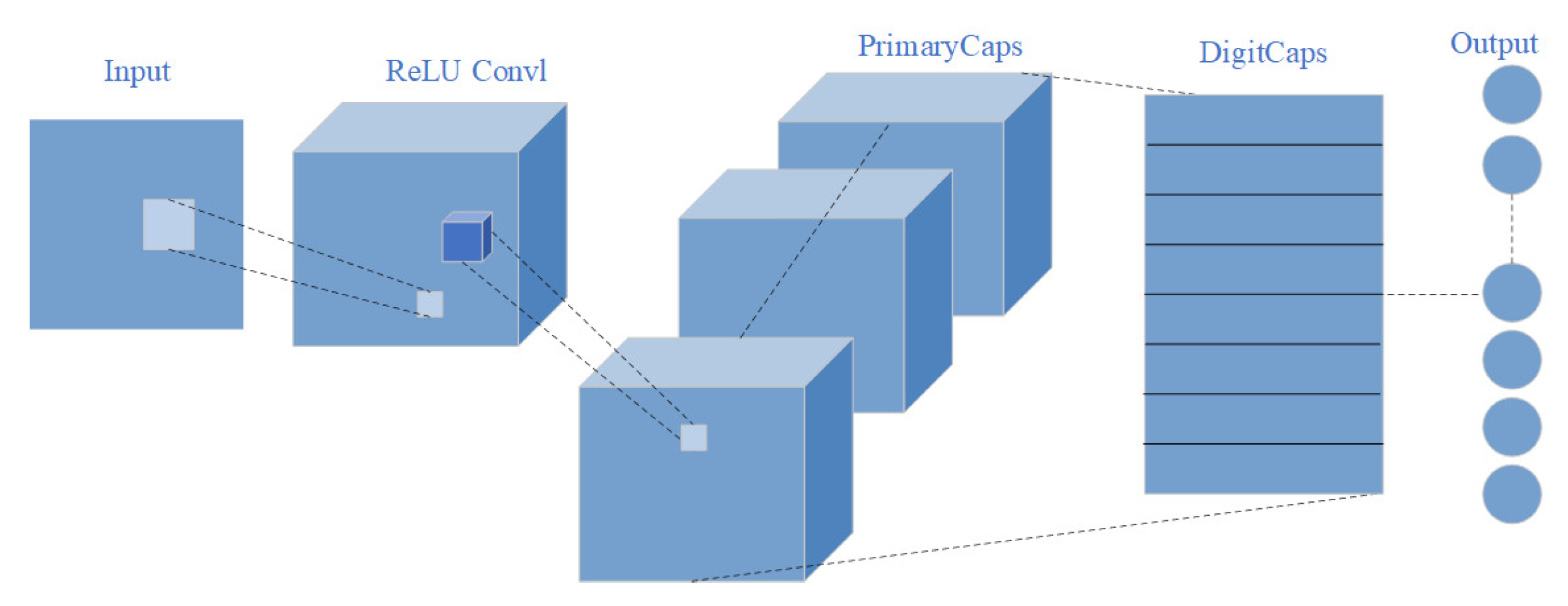
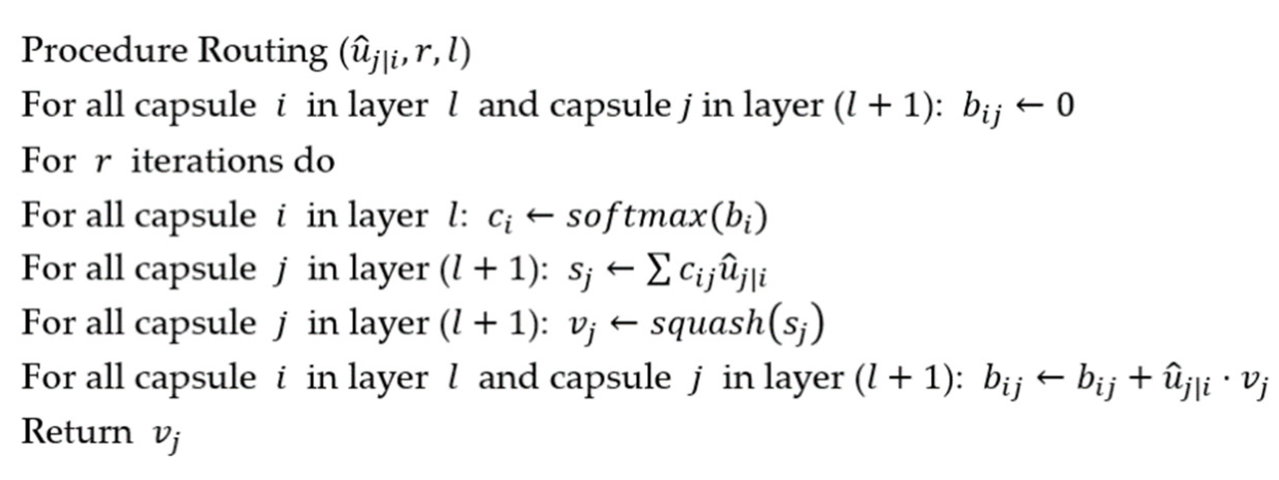
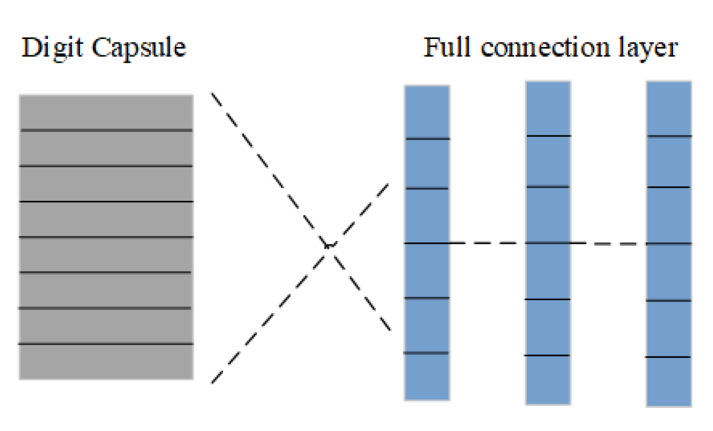
2.1. Capsule Network

The CapsNet model proposed by Hinton et al. is also called the vector capsule network. Since the vector is selected as the capsule and the output of the network is also a vector, the direction of the vector can be used to represent the existence of the target, and the length of the vector can represent the characteristics of the target. CapsNet is a high-performance neural network classifier that consists of a convolution layer, a primary capsule layer, and a digital capsule layer. The structure of the entire CapsNet is shown in Figure 1.

The network structure consists of three parts. The first part is the conventional convolution operation between the input layer and convolution layer, the second part is the primary capsule generation operation between the convolution layer and primary capsule layer, and the third part is the advanced capsule generated between the primary capsule layer and the digit capsule layer. When constructing the primary capsule, the scalar fault features extracted from the convolution layer are arranged into vector fault features, and the primary capsule u_i is generated, where i represents the i-th fault characteristic capsule. Information communication between the digital capsule layer and the primary capsule layer occurs through dynamic routing. The calculation method of dynamic routing determines the dynamic connection between the high-level and low-level hidden layers, so the model can automatically screen more effective capsules to improve performance; the pseudo code of dynamic routing algorithm [12] is shown in Figure 2.

Step 1: Multiply the primary capsule and the weight matrix to obtain the example prediction capsule. The mathematical formula is as follows:

$${\hat{u}}_{j|i}=w_{ij}{u}_i$$

(1)

In Formula (1), i represents the primary capsule label, j is the digital capsule label, u_i is the input vector of the primary capsule layer, which represents the low-level feature of the fault data in the input layer, such as the single fault attribute of the fault data. ${\hat{u}}_{j|i}$ is an example prediction capsule, which represents a high-level feature j derived from low-level feature i, and w_ij is the weight matrix, which contains the connection relationship between the low-level feature and the high-level feature, for example, the relationship between different fault attributes of fault data.

Step 2: Calculate the coupling coefficient between the example prediction capsule and the digital capsule through Formula (2) and calculate the weighted sum of all the example prediction capsules to obtain the digital capsule.

$$c_{ij}=\exp \left(b_{ij}\right)/{\displaystyle \sum }_j\exp (b_{ij})$$

(2)

$$s_j={\displaystyle \sum }_j{c}_{ij} {\hat{u}}_{j|i}$$

(3)

In Formulas (2) and (3), c_ij and b_ij respectively represent the coupling coefficient and a priori connection weight between the example prediction capsule ${\hat{u}}_{j|i}$ and the digital capsule s_j. The initial values of b_ij are all 0, ∑ c_ij = 1 and c_ij is updated via dynamic routing, which determines which high-level capsules a low-level capsule is sent to.

Step 3: Compress the length of the digital capsule s_j to [0, 1] based on the squash function of Formula (4), and the digital capsule layer is obtained. Output the digital capsule v_j and update the prior connection weight b_ij.

$$v_j=squash\left(s_j\right)=\frac{\Vert s_j{}^2\Vert }{1+\Vert s_j{}^2\Vert }\cdot \frac{s_j}{\Vert s_j{}^2\Vert }$$

(4)

$$b_{ij}\leftarrow b_{ij}+{\hat{u}}_{j|i}·v_j$$

(5)

The vector transfer between low-layer and high-layer capsules is realized by dynamic routing, and the correlation is measured by a scalar product. The length of the vector represents the existence of an entity, and key features such as spatial position are constructed.

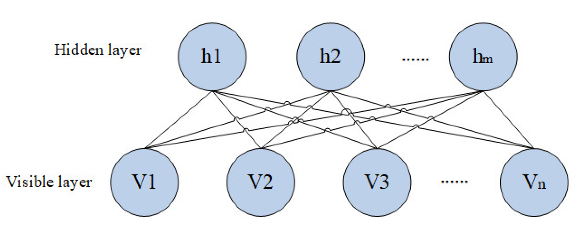
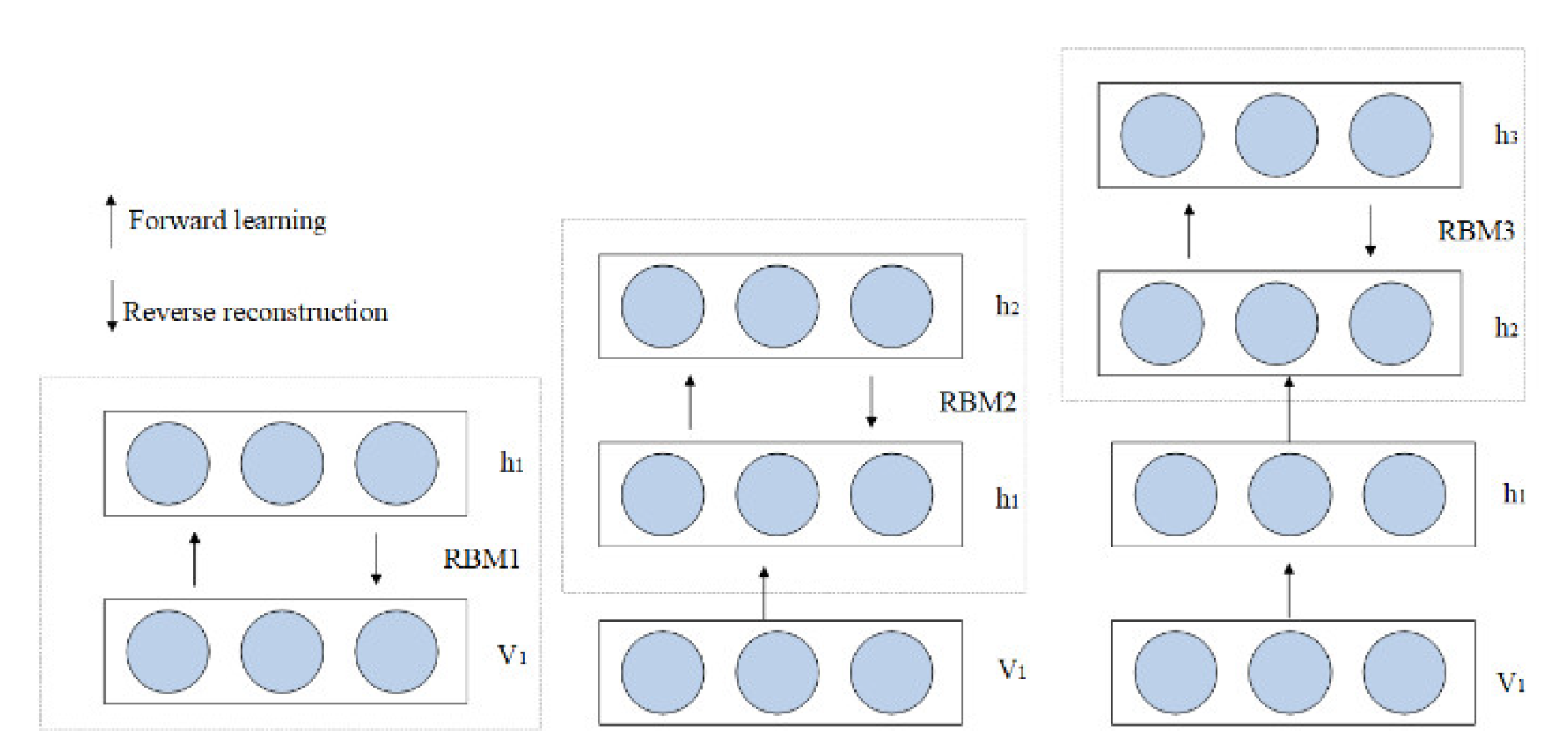
2.2. Deep Belief Network

A DBN is a neural network model consisting of a multiple restricted Boltzmann machine (RBM) [24], the core RBM unit is an energy-based model, and the structure diagram is shown in Figure 3.

The energy of the RBM system determined by state (v, h) can be expressed as:

$$E\left(\mathit{v},\mathit{h}|\theta \right)=-{\displaystyle \sum }_{i=1}^n{a}_i{v}_i-{\displaystyle \sum }_{j=1}^m{b}_j{h}_j-{\displaystyle \sum }_{i=1}^n{\displaystyle \sum }_{j=1}^m{v}_i{w}_{ij}{h}_j$$

(6)

In Formula (6), θ = (w_ij, a_i, b_i) is the RBM parameter, n and m are the number of neurons in the visible and hidden layers, v is the input unit vector of the visible layer, and v_i is the state of neuron i in the visible layer. Its bias value is set as a_i. h is the output unit vector of the hidden layer, h_j is the state of the hidden layer neuron j, and the bias value is b_j. The connection weights of neurons i and j are defined as w_ij.

The joint probability distribution of (v, h) can be obtained from Formula (7):

$$p\left(\mathit{v},\mathit{h}|\theta \right)=\exp \left(-E\left(\mathit{v},\mathit{h}|\theta \right)\right)/{{\displaystyle \sum }}_{\mathit{v},\mathit{h}}\exp \left(-E\left(\mathit{v},\mathit{h}|\theta \right)\right)$$

(7)

The marginal probability distribution of $\mathit{v},\mathit{h}$ can be obtained by Formulas (8) and (9):

$$p\left(\mathit{v}|\theta \right)={{\displaystyle \sum }}_{\mathit{h}}\exp \left(-E\left(\mathit{v},\mathit{h}|\theta \right)\right)/{{\displaystyle \sum }}_{\mathit{v},\mathit{h}}\exp \left(-E\left(\mathit{v},\mathit{h}|\theta \right)\right)$$

(8)

$$p\left(\mathit{h}|\theta \right)={{\displaystyle \sum }}_{\mathit{v}}\exp \left(-E\left(\mathit{v},\mathit{h}|\theta \right)\right)/{{\displaystyle \sum }}_{\mathit{v},\mathit{h}}\exp \left(-E\left(\mathit{v},\mathit{h}|\theta \right)\right)$$

(9)

When $h_j=1$ or $v_i=1$, the conditional probability function is:

$$p\left(h_j=1|v,\theta \right)=sigm(b_j+{\displaystyle \sum }_{i=1}^n{v}_i{w}_{ij})$$

(10)

$$p\left(v_i=1|h,\theta \right)=sigm(a_i+{\displaystyle \sum }_{j=1}^m{w}_{ij}{h}_j)$$

(11)

In Formulas (10) and (11), sigm is the activation function.

DBN feature extraction is a layer-by-layer learning process of multiple RBMs, including forward learning and reverse reconstruction. DBNs can map complex signals to output and has good feature extraction ability [25]. The layer-by-layer learning process is shown in Figure 4.

DBN solves the optimization problem of deep-level neural network by using layer-by-layer training method, and gives the whole network a better initial weight by layer-by-layer training, meaning that the network can reach the optimal solution as long as it is fine-tuned.

3. DBN-CapsNet Fault Diagnosis Method

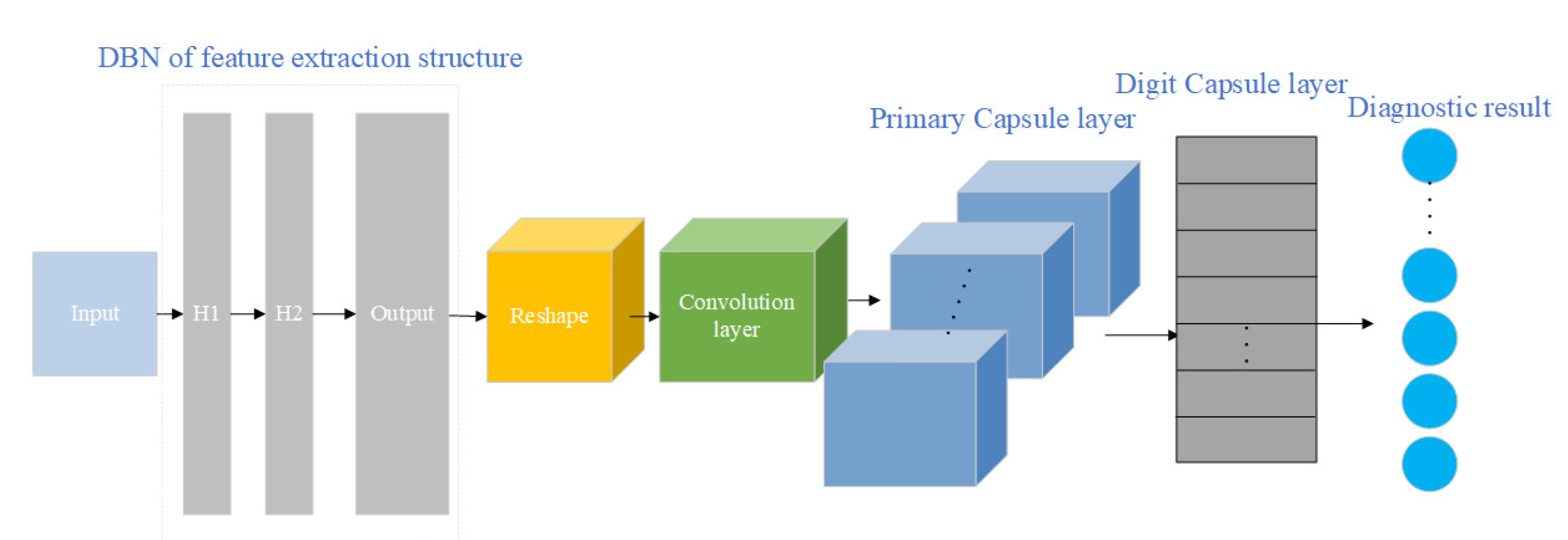
3.1. Structure of DBN-CapsNet

To improve the feature extraction ability of CapsNet for fault data, DBN is used to improve the single convolution structure of CapsNet and build a more comprehensive and rich feature extraction unit. Combined with the primary capsule structure and digital capsule structure, a DBN improved capsule network (DBN-CapsNet) model is proposed, and its structure is shown in Figure 5.

The input data of DBN-CapsNet are the historical fault data information of smart meters after one-hot encoding. The front end of the network adopts a double hidden layer DBN structure and convolution layer for feature extraction. DBN can also solve the problem of high data dimensions and sparse data due to one-hot encoding. The reshape layer transforms the output of the DBN into the input suitable for the convolution layer, which ensures the sufficiency of information extraction, and the function of feature acquisition is obvious. The back end adopts a capsule structure to construct vector neurons. The primary capsule stores low-level features, and the digital capsule stores high-level features. Transmission from the primary capsule to the digital capsule relies on the dynamic routing algorithm, and fault diagnosis is realized by dynamic routing. The number of vectors of the digital capsule is the number of fault types of the smart meter, and the norm of each vector of the digital capsule forms the output vector, which corresponds to the probability of the occurrence of different fault types. The fault type corresponding to the vector with the largest norm value is the final diagnosis result.

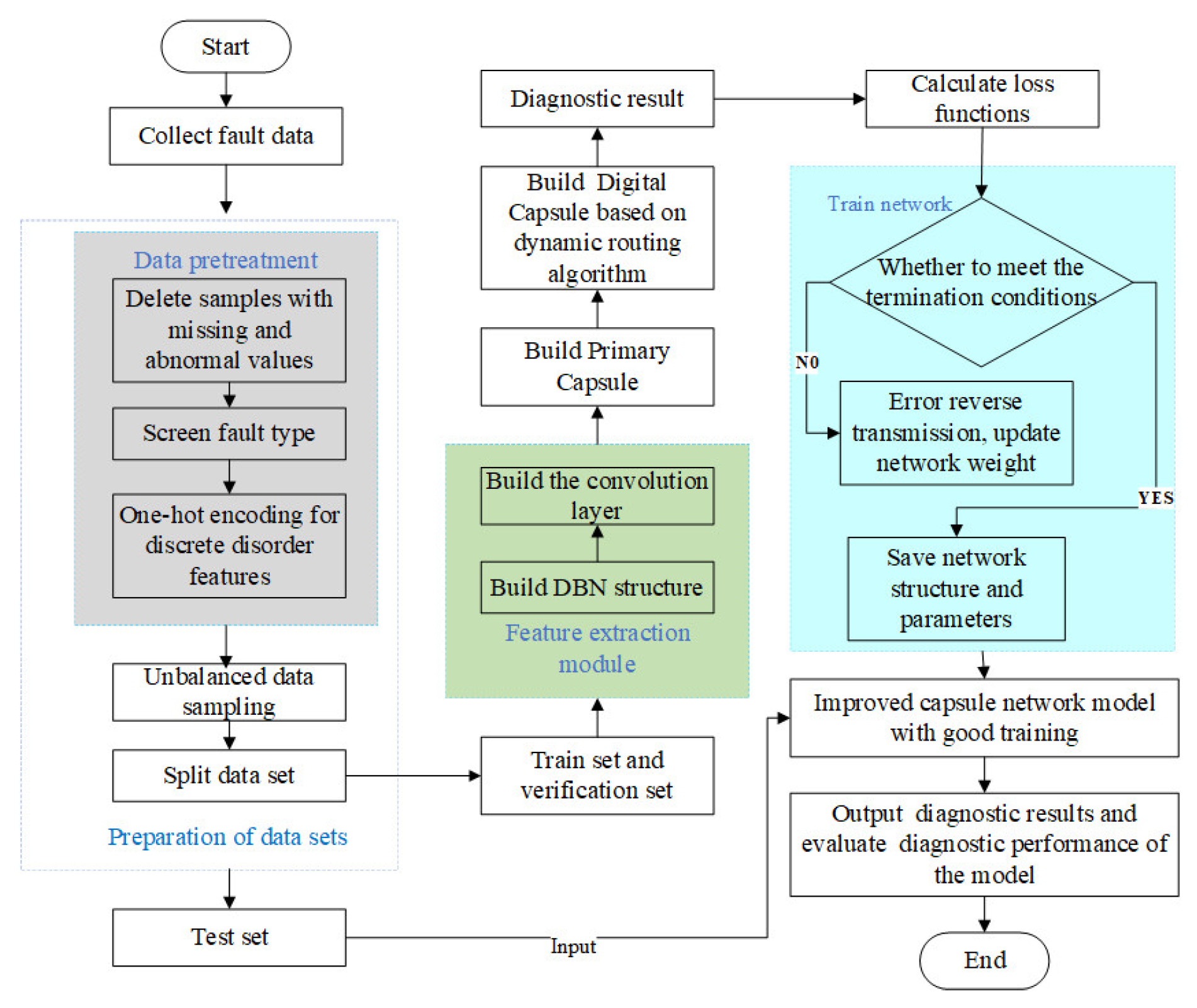
3.2. Fault Diagnosis Process

The smart meter fault diagnosis process based on the DBN-CapsNet model is shown in Figure 6.

Step 1: Collect smart meter fault data.

Step 2: Pre-process the fault sample data. Fault samples with missing values are deleted; whether each attribute could be used as the input of the fault diagnosis model is judged; the fault types of the samples are analyzed statistically to screen the fault types; and one-hot encoding is used to encode the discrete and disordered attributes [26].

Step 3: Conduct an unbalanced data sampling and dataset dividing. The mixed sampling method of oversampling and undersampling is adopted [27]. Random sampling for fault types that need undersampling and SMOTE (Synthetic Minority Over-Sampling Technique, SMOTE) sampling for fault types that need oversampling are conducted [28]. The formula for determining the theoretical sample size of each fault type after sampling is as follows:

$$N\text{\_}ne{w}_i=\{\begin{array}{c}{N}_i-a\ast \left(N_i-N_{mean}\right) \left(undersampling\right)\\ N_i+a\ast \left(N_{mean}-N_i\right) \left(oversampling\right)\end{array},i=1,2,\dots M$$

(12)

Suppose there are M fault types in the fault dataset of smart meters, $N\text{\_}ne{w}_i$ is the sample size of type $i$ after sampling, $N_i$ is the sample size of type $i$ before sampling, and $a$ is the sample balance coefficient. Here, $a=0.5$, and $N_{mean}$ represents the mean value of the sample size of all fault types before sampling. If $N_i$ is greater than $N_{mean}$, the undersampling method should be adopted; otherwise, the oversampling method should be adopted.

The dataset is divided into a training set, verification set and test set. The first two are used to train the parameters of the DBN-CapsNet model, and the test set is used to evaluate the performance of the DBN-CapsNet fault diagnosis model.

Step 4: Build the DBN structure and convolution layer and set network parameters to realize fault feature extraction.

Step 5: Construct the primary capsule and the digital capsule based on the dynamic routing algorithm.

Step 6: Train the DBN-CapsNet model. The back propagation algorithm is used to complete the training of DBN-CapsNet, including two processes: forward excitation propagation and back weight update. In the process of forward excitation propagation, the input features are transmitted to the output layer after being processed by the DBN layer, convolution layer and capsule layer, and the loss function value (error) is calculated through the diagnostic results and actual results. In the process of back weight updating, first, the chain rule is used to transfer the error from the output layer to the middle layer. Then, the weight of each layer is updated by the gradient descent method. When the predetermined epoch is reached, the training is stopped.

Because CapsNet allows multiple types to exist at the same time, the traditional cross-entropy loss cannot be used directly. An alternative is to use the margin loss function, which is expressed as:

$$L_k=T_k\cdot \max {\left(0,m^{+}-\Vert v_k\Vert \right)}^2+\lambda \left(1-T_k\right)max{\left(0,\Vert v_k\Vert -m^{-}\right)}^2$$

(13)

$k$ is the number of types; $v_k$ represents the output vector of type $k$; $L_k$ represents the loss of type $k$; $T_k$ is the indicator function of classification (1 for existence and 0 for nonexistence); $m^{+}$ is the upper bound, punishing false-positive, that is, the existence of type $k$ is predicted but it does not exist; $m^{-}$ is the lower bound, punishing false negative, that is, type $k$ is predicted to not exist but it does exist; and $\lambda$ is the proportion coefficient, which adjusts the proportion of the two. Here, $m^{+}=0.9, m^{-}=0.1$, and $\lambda =0.5$.

The meaning of reconstruction is to build the actual data of this type with the predicted type. The reconstruction loss is calculated by constructing a three-layer connecting layer after the digit capsule layer. As shown in Figure 7, we obtained the reconstructed output data and calculated the sum of the square of the distance between the actual data and the output data as the loss value.

Overall loss = Margin loss + α* Reconstruction loss, where α = 0.01 and margin loss is dominant.

Step 7: The diagnostic performance of the DBN-CapsNet model is evaluated by the test set, and the diagnostic results are output. The confusion matrix is an important tool to evaluate the performance of the classification model. It can be used to calculate the accuracy rate ($A$), precision rate ($P$), recall rate ($R$) and F value. As shown in Figure 8, suppose there are $k$ fault types, and $n_{ij}$ represents the number of samples that diagnose type $i$ as type $j$.

$$A={{\displaystyle \sum }}_{i=1}^k{n}_{ii}/{{\displaystyle \sum }}_{i=1}^k{{\displaystyle \sum }}_{j=1}^k{n}_{ij}$$

(14)

$$P_i=n_{ii}/{{\displaystyle \sum }}_{j=1}^k{n}_{ji}$$

(15)

$$R_i=n_{ii}/{{\displaystyle \sum }}_{j=1}^k{n}_{ij}$$

(16)

$$F_i=2P_i{R}_i/(P_i+R_i)$$

(17)

$$Macro F1=\frac{1}{k}{{\displaystyle \sum }}_{i=1}^k{F}_i$$

(18)

As seen from Formula (14), the accuracy rate is a measure of the average accuracy of the overall diagnosis. For the multiclassification problem, the precision rate $P$, recall rate $R$ and F value should also be considered. The precision rate is the accuracy of the classification model for a certain type, and the recall rate is the coverage of the classification model for a certain type. The F value is a measure of the accuracy and coverage of the classification model for a certain type, and it is a harmonic average of the precision and recall. Macro F1 combines the two indicators of precision rate and recall rate, so accuracy rate and Macro F1 are used as the evaluation indicators of model diagnosis performance.

4. Example Verification

4.1. Fault Dataset Preparation of Smart Meter

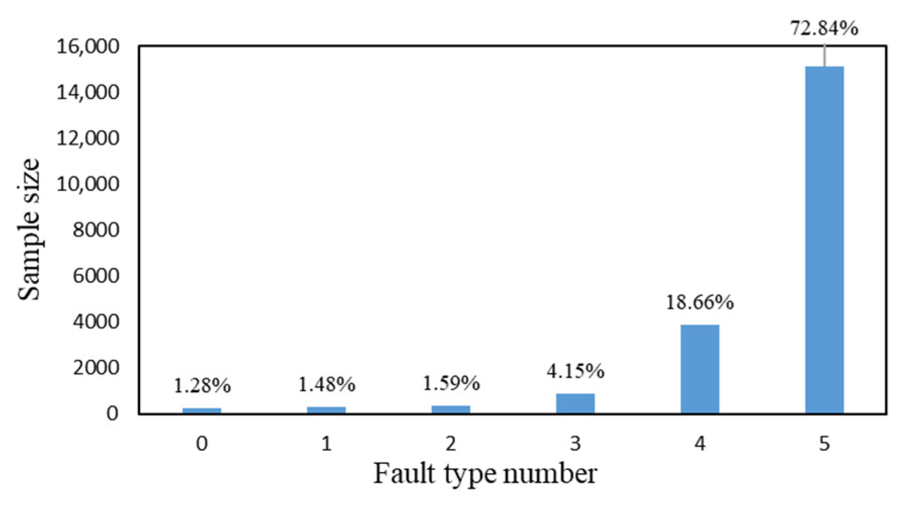
4.1.1. Introduction of Dataset

At present, the data center of the power grid system collects the operation data of the smart meter every day. The fault data information includes the manufacturer, equipment type, asset number, operation date, equipment status, fault discovery date, fault source, working time, power supply unit, equipment specification, communication mode and other related attributes of the failed smart meter. Due to the large number of smart meter suppliers, the internal design and components of different smart meters are also different. Therefore, smart meters often show family defects, and smart meters of the same batch from the same manufacturer are more likely to have the same type of fault. An increase in the working time will reduce the reliability of smart meters. Smart meters have a certain life expectancy, and with increasing working time, the ageing of their components and battery wear-out will cause smart meters to be more prone to failure, for example, error over tolerance, capacitor damage, battery damage and other hardware damage. Attributes of the dataset that are obviously independent of the fault type are deleted, the current attributes are integrated, and finally the attributes that affect the fault type are retained, including 10 attributes: equipment type, equipment status, equipment specification, communication mode, manufacturer, power supply unit, fault source, put into operation month, fault month, and normal operation duration (years).

4.1.2. Data Pretreatment

First, the samples with missing data are eliminated, and then the fault types of samples are analyzed statistically. Some fault types have too few samples (sample size is less than 100), so we do not perform an in-depth study and delete the relevant sample data. The remaining fault types are numbered 0–5 in ascending order of the sample size. In the remaining sample data, there are attributes represented by the text such as equipment type, equipment status, equipment specification, communication mode, manufacturer, power supply unit and fault source; these attributes are discrete and unordered. In this paper, the one-hot encoding method is used to digitize these attributes to better carry out the following deep learning (the three attributes of put into operation month, fault month, and normal operation duration do not need one-hot encoding). The distribution histogram of the size of the failure samples is drawn, as shown in Figure 9.

From Figure 9, the size of samples of each fault type is not balanced, as fault type 4 and 5 account for a large proportion, totaling nearly 92%, while fault type 0 to type 3 account for only approximately 8%. An imbalance in the sample size will affect the result of fault diagnosis and the classification model will ignore small sample types. Therefore, this paper adopts the mixed sampling method of oversampling and undersampling, i.e., random sampling for fault types that require undersampling and SMOTE sampling for fault types that require oversampling. The sample size after mixed sampling of unbalanced data is shown in

Table 1. Sample size before and after sampling.

Fault Type Number	Fault Type	Sample Size before Sampling	Sample Size after Sampling	Proportion after Sampling
0	Overload burn-out meter	267	1865	8.97%
1	Battery failure	307	1885	9.07%
2	Pulse sampling failure	330	1897	9.13%
3	Clock out of order	863	2163	10.41%
4	Communication failure	3879	3671	17.66%
5	Electromechanical failure	15,142	9303	44.76%
Mean		3464	/

.

As shown in Table 1, comparing the sample proportion before and after sampling, the sample proportion after using the mixed sampling method proposed in this paper is significantly more balanced than that before sampling, and the gap between sample sizes is significantly reduced.

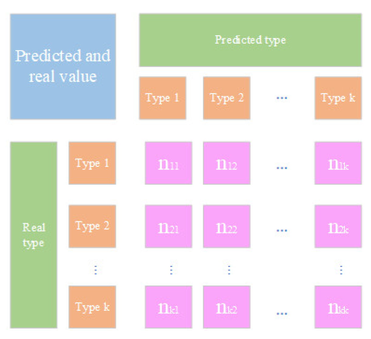
4.2. Performance Verification of DBN-CapsNet Fault Diagnosis

4.2.1. DBN-CapsNet Network Structure and Parameter Settings

To improve the fault diagnosis accuracy of smart meters, it is necessary to probe and search for the best network structure and parameters before training and improving the capsule network. After data processing and one-hot encoding, the input layer is a 1 × 136 vector and a double hidden layer DBN network structure composed of RBM1 and RBM2 is established; the last three column vectors do not need to be input into DBN, and these are added to the final output of DBN. A capsule network consisting of a convolution layer and capsule layer is established. Since there are six fault types in smart meters, the output layer is a 1 × 6 vector, which represents the fault types of input samples. The number of epochs for the network training was 350, the batch size was 200, the Adam algorithm was selected for the optimizer, the learning rate was 0.01, and the number of iterations of dynamic routing was set to three. The specific DBN-CapsNet network structure and parameter settings are shown in

Table 2. Network structure and parameter settings of DBN-CapsNet.

Layers	Structure and Parameters	Output Size
1	Input layer	$1\times 136$
2	DBN structure: Number of RBM1 hidden neurons: 100 Number of RBM2 hidden neurons: 80 Number of neurons in DBN output layer: 61	$1\times 64$
3	Reshape layers	$1\times 8\times 8$
4	Convolution layer: 56 convolution kernels, the size of convolution kernels is $3\times 3$, and the activation function is ReLU.	$6\times 6\times 56$
5	Primary capsule: the output channel is 56, the capsule dimension is 8, and the convolution kernel size is $3\times 3$.	$4\times 4\times 8\times 56$
6	Digit capsule: the number of output capsules is 6, the dimension of output capsules is 16, and the activation function is Squash.	$6\times 10$
7	Output layer	1 × 6

.

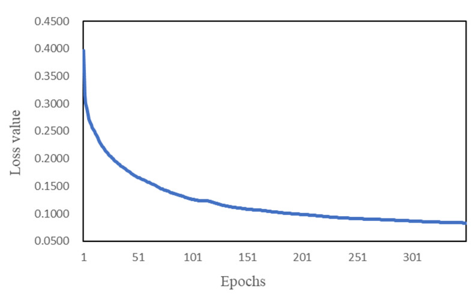
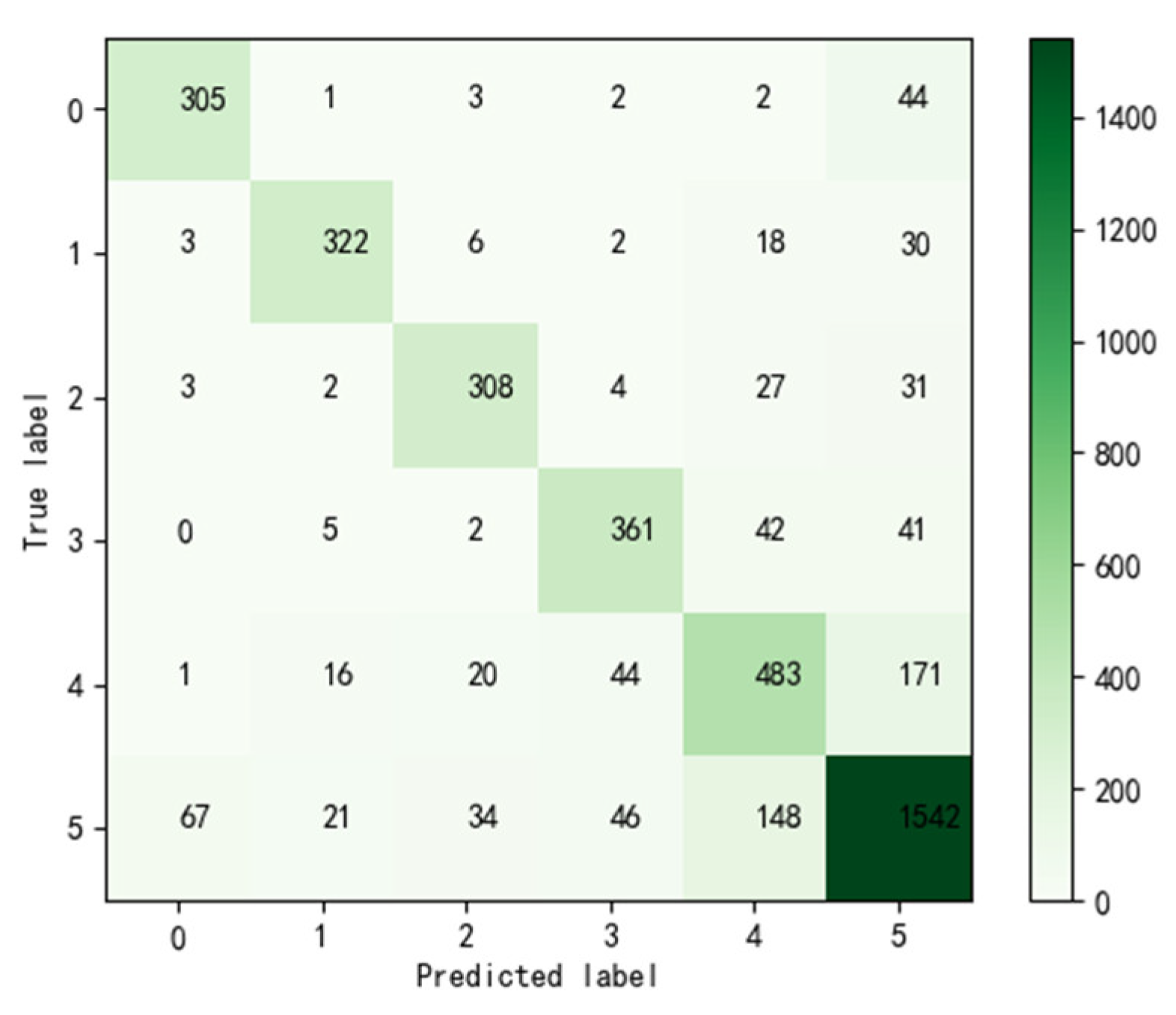
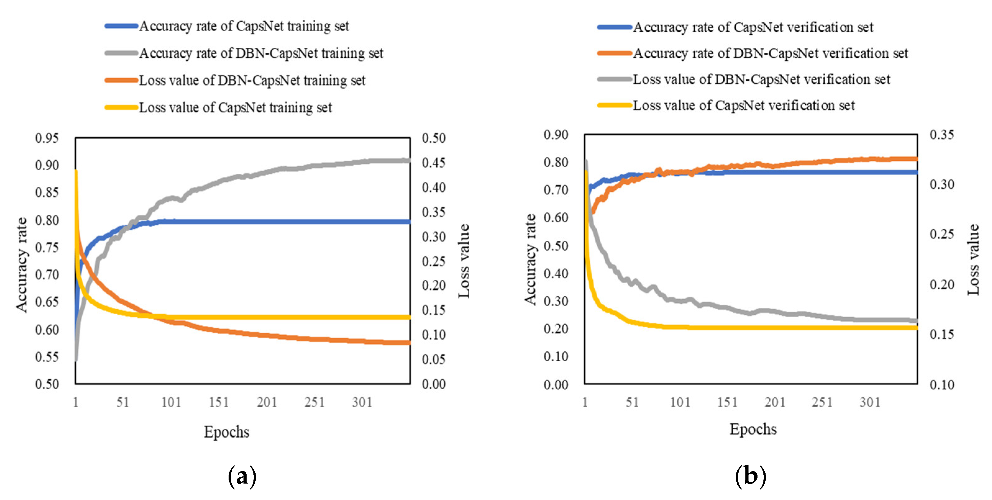
4.2.2. Model Training and Diagnosis Result Analysis

During the experiment, 80% of the smart meter fault dataset is used as the training dataset and 20% is taken as the test dataset. To avoid the randomness of the experimental results caused by the randomness of dataset division, the dataset is randomly divided and trained five times, and the median value of its diagnostic results is taken as the final experimental result. The training dataset is used to train the model with hierarchical 10-fold cross validation [4]. The main purpose of randomly selecting 10% of the training set as the verification set is to prevent the model from overfitting the training samples and losing the ability to fit to and predict other data to ensure the reliability of the results of the classification model. Then, the test dataset is used to validate the trained model.

The method of the proposed method runs under PyCharm software, and the depth learning framework uses TensorFlow 2.6.0 and Keras 2.6.0. The computer hardware configuration is AMD Ryzen7 4800U with Radeon Graphics (16 CPUs), 1.8 GHz. The model training results are as follows:

As shown in Figure 10, the loss function value of the training set decreases with increasing epochs. When the epoch reaches 300, the value of the loss function of DBN-CapsNet tends to be stable, which shows that DBN-CapsNet has converged. When the epoch reaches 350, the loss value is 0.08, the trained DBN-CapsNet is used for subsequent fault diagnosis tasks. The fault diagnosis results of the model are shown in Figure 11.

We calculate the precision rate, recall rate and F value according to Figure 11, and the results are shown in the

Table 3. Precision rate, recall rate and F value of DBN-CapsNet diagnostic results.

Fault Type Number	Precision Rate	Recall Rate	F Value
0	0.80	0.85	0.83
1	0.88	0.85	0.86
2	0.83	0.82	0.82
3	0.79	0.80	0.79
4	0.67	0.66	0.66
5	0.83	0.83	0.83

.

As seen from Table 3, DBN-CapsNet has a good diagnostic effect for fault types 0, 1, 2, and 5 with precision rates, recall rates and F value above 0.8, and the fault type numbered 4 is poor. As seen from the Figure 11, communication failure is easily misdiagnosed as electromechanical failure. Mainly because the external manifestations of these faults are similar, it is difficult to judge directly and accurately through the characteristic attributes of the fault dataset, and the maintenance personnel need to diagnose the faulty smart meter further professionally. Some factors affecting the fault diagnosis performance of the model are analyzed below:

(1) The effect of the size of the batch on the diagnostic performance of DBN-CapsNet was analyzed. The batch size is the number of samples required for each round of training. The batch size was set as 50, 100, 200, 300, 400 and 500 for simulation, and the evaluation indicators were counted. As shown in

Table 4. Results under different batch size.

Batch Size	Accuracy Rate	Macro F1	Training Time (s)
50	0.7958	0.7950	4775
100	0.7967	0.7950	3886
200	0.7989	0.7983	3779
300	0.7811	0.7783	3603
400	0.7746	0.7700	3522
500	0.7768	0.7700	3449

, with increasing batch size, the accuracy rate of DBN-CapsNet and Macro F1 first increased and then decreased. When the batch size is 200, DBN-CapsNet has the highest accuracy rate and Macro F1, indicating the best performance for fault diagnosis. In terms of time, increasing the batch size can speed up the training speed, but it will affect the generalization ability of the network and lead to the degradation of fault diagnosis performance. In summary, the batch size should be determined according to the size of the dataset and the performance of the computer. In this paper, the batch size is set to 200 to achieve high performance for DBN-CapsNet.

(2) The influence of optimizer selection on DBN-CapsNet diagnostic performance is analyzed. Different optimizers are set up and simulated. The evaluation indicators are shown in

Table 5. Results under different optimizers.

Optimizer	Accuracy Rate	Macro F1
SGD	0.4472	0.1033
RMSprop	0.7912	0.7917
Adagrad	0.6250	0.5233
Adadelta	0.4472	0.1033
Adamax	0.7667	0.7533
Adam	0.7989	0.7983

. When Adam, RMSprop and Adamax are used as optimizers, the improved capsule network has better performance. The accuracy rate and Macro F1 indicators of the Adam algorithm are higher than those of the other five optimizers, and the performance of fault diagnosis is the best. Further observation shows that the corresponding indicators of the Adagrad, SGD, and Adadelta algorithms are lower than 0.65, indicating that these optimizers of DBN-CapsNet are not suitable for the fault diagnosis task of smart meters.

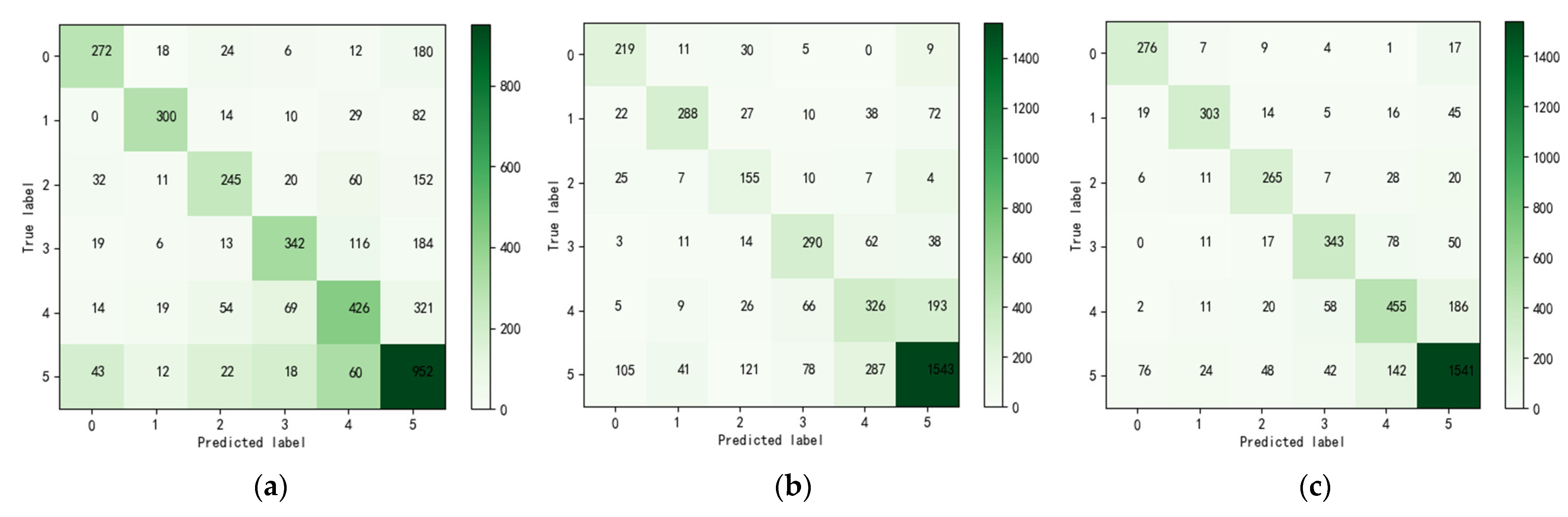
4.2.3. Comparative Analysis of Algorithms

To prove the effectiveness of the DBN-CapsNet method proposed in this paper in the fault diagnosis of smart meters, this paper uses a machine learning algorithm support vector machine (SVM), one-dimensional CNN and traditional CapsNet to learn the historical fault data of smart meters.

SVM: Use the svm.SVC function in the Sklearn library to realizes the fault diagnosis of smart meters based on SVM method. The penalty parameter $C$ is set to 0.1, the kernel is set to rbf, the gamma is set to 0.1, and the maximum iteration is 1000.

CNN: The best parameters and structure of the convolutional neural network are determined by the trial method, and the features are extracted by six layers Conv1D, the number of convolution kernels is 12, 12, 48, 48, 64, 64, and the size of convolution kernels is 12, 12, 12, 3, 3, 3. A layer of Max Pooling 1D is added after every two layers of Conv1D to retain the main features, and the tanh function is used as the activation function for each layer of convolution. The output layer has six nodes and the activation function is SoftMax. The cross-entropy loss function is used as the loss function for model training, with epochs of 500 and a batch size of 200; the optimizer is the Adam algorithm.

CapsNet: Compared with DBN-CapsNet, the traditional capsule network has no DBN structure, and the other network structures and setting parameters are the same as DBN-CapsNet.

These models are trained several times, and the results are shown in Figure 12.

We calculate the precision rate (P), recall rate (R) and F value according to Figure 12, and the results are shown in the

Table 6. The precision rate, recall rate and F value of CapsNet, CNN and SVM.

Fault Type Number	CapsNet			CNN			SVM
	P	R	F Value	P	R	F Value	P	R	F Value
0	0.73	0.88	0.80	0.58	0.80	0.67	0.72	0.53	0.61
1	0.83	0.75	0.79	0.78	0.63	0.70	0.82	0.69	0.75
2	0.71	0.79	0.75	0.42	0.75	0.53	0.66	0.47	0.55
3	0.75	0.69	0.72	0.63	0.69	0.66	0.74	0.50	0.60
4	0.63	0.62	0.63	0.45	0.52	0.48	0.61	0.47	0.53
5	0.82	0.82	0.83	0.83	0.71	0.76	0.51	0.86	0.64

.

According to Table 6, the predictive effect of SVM and CNN is not as good as that CapsNet, and the accuracy rate and Macro F1 of the corresponding algorithm are compared, as shown in

Table 7. Comparison of the results of different algorithms.

Algorithm	Accuracy Rate	Macro F1	Training Time (s)
SVM	0.61	0.61	210
CNN	0.68	0.63	939
CapsNet	0.77	0.75	12,134
DBN-CapsNet	0.80	0.80	3779

.

As seen in Table 7, SVM has the shortest training time, but its diagnosis effect is the worst, which shows that the deep learning method is more suitable for the fault diagnosis of smart meters than the machine learning algorithm SVM. The DBN-CapsNet training time is much longer than the CNN training time; however, its diagnostic effect is better than that of CNN, and the accuracy rate and Macro F1 value are improved by 12% and 17% respectively. CNN and CapsNet both used convolutional layers to extract the features of input data in the early stage, and in the later stage, they used pooling layers and capsule layers to map the complex nonlinear relationship between features and fault types of smart meters. The performance of CapsNet is better than that of CNN, which shows that CNN will lose some characteristic information in the pool operation, which limits the precision of fault diagnosis. However, the capsule layer and dynamic routing algorithm of CapsNet can deeply mine the relationship between features and fault types and more accurately diagnose the fault types of smart meters. DBN-CapsNet is a further optimization of the feature extraction part of CapsNet. It can be seen from the results in Table 7 that compared with CapsNet, the diagnostic accuracy rate of DBN-CapsNet and the Macro F1 value were improved by 3% and 5%, respectively, and the training time was significantly shortened. This also shows that the improved capsule network based on DBN can capture more comprehensive and effective feature information, improve the network training efficiency, and improve the performance of fault diagnosis.

As shown in Figure 13, in the training set, the loss value of CapsNet decreases faster than that of DBN-CapsNet before 100 epochs, and the loss value is stable around 0.13 after 150 epochs. However, when DBN-CapsNet iterates to 300 epochs, the loss value is stable to around 0.08. The accuracy rate of CapsNet is about 80%, while that of DBN-CapsNet is about 90%, which shows that CapsNet has a fast convergence speed and tends to be stable quickly, but the feature extraction ability is limited and the accuracy rate of fault diagnosis is not high. The convergence speed of DBN-CapsNet is relatively slow, but with the increase in the number of iterations, the accuracy rate of fault diagnosis gradually increases, which is 10% higher than that of CapsNet. In the verification set, the loss value of CapsNet decreases faster than that of DBN-CapsNet and is a little smaller than that of DBN-CapsNet, but the fault diagnosis accuracy rate of CapsNet is lower than that of DBN-CapsNet. The accuracy rate of DBN-CapsNet is finally around 0.8, and the accuracy rate of DBN-CapsNet fault diagnosis model in the test set is also 0.8, indicating that the diagnosis performance of DBN-CapsNet is stable and has a good diagnosis effect.

5. Conclusions

This paper presents a model of smart meters fault diagnosis based on a DBN improved capsule network (DBN-CapsNet). We improve the data quality by means of statistical sample size distribution, screening fault types, selecting fault characteristic attributes and one-hot encoding method to meet the needs of building fault diagnosis model. We adopt the mixed sampling method of undersampling and oversampling to solve the problem of unbalanced sample size distribution, and a DBN-CapsNet smart meter fault diagnosis model is built. The effects of batch size, optimizer, and iteration times of capsule network on the diagnostic performance of smart meters are discussed. Finally, the comparative experiments show that the proposed method has better diagnostic performance than SVM and CNN. Compared with CapsNet, the improved capsule network can improve the feature extraction and fault diagnosis ability by combining DBN with a convolution layer structure, DBN also solves the problem of high data dimensions and sparse data due to one-hot encoding, the accuracy rate and Macro F1 were improved by 3% and 5% respectively, and the training time for the model was significantly reduced.

References

1. Xiong, D.Z.; Jiang, T.H.; Chen, X.Q.; Chen, Y.L. Development of intelligent checking device for power information collection fault. Electr. Meas. Instrum. 2019, 56, 120–123. [Google Scholar] [CrossRef]
2. Zhou, F.; Cheng, Y.Y.; Du, J.; Feng, L.; Xiao, J.; Zhang, J.M. Construction of Multidimensional Electric Energy Meter Ab-normal Diagnosis Model Based on Decision Tree Group. In Proceedings of the 2019 IEEE 8th Joint International Information Technology and Artificial Intelligence Conference (ITAIC), Chongqing, China, 24–26 May 2019. [Google Scholar]
3. Li, N.; Fei, S.J.; Liu, G.L.; Yang, L. Fault Traceability of Metering Device Based on Deep Belief Network. Smart Power 2020, 48, 118–124. [Google Scholar]
4. Gao, X.; Diao, X.P.; Liu, J.; Zhang, M.; Yang, H. A Multi-classification Method of Smart Meter Fault Type Based on Model Adaptive Selection Fusion. Power Syst. Technol. 2019, 43, 1955–1961. [Google Scholar] [CrossRef]
5. Xue, Z.; Sun, Y.; Dong, Z.C.; Fang, Y.J. Fault diagnosis method of power consumption information acquisition system based on fuzzy Petri nets. Electr. Meas. Instrum. 2019, 56, 64–69. [Google Scholar] [CrossRef]
6. Guo, X.C.; Liu, B.B.; Wang, L.L. Fault Diagnosis of Mining Power Cable Based on Waveletpacket and Cs-Bp Neural Network. Comput. Appl. Softw. 2021, 38, 105–110. [Google Scholar] [CrossRef]
7. Wen, L.; Li, X.; Gao, L.; Zhang, Y. A New Convolutional Neural Network-Based Data-Driven Fault Diagnosis Method. IEEE Trans. Ind. Electron. 2018, 65, 5990–5998. [Google Scholar] [CrossRef]
8. Shao, H.; Jiang, H.; Lin, Y.; Li, X. A novel method for intelligent fault diagnosis of rolling bearings using ensemble deep auto-encoders. Mech. Syst. Signal Process. 2018, 102, 278–297. [Google Scholar] [CrossRef]
9. Orrù, P.; Zoccheddu, A.; Sassu, L.; Mattia, C.; Cozza, R.; Arena, S. Machine Learning Approach Using MLP and SVM Algorithms for the Fault Prediction of a Centrifugal Pump in the Oil and Gas Industry. Sustainability 2020, 12, 4776. [Google Scholar] [CrossRef]
10. Wu, N.; Wang, Z. Bearing Fault Diagnosis Based on the Combination of One-Dimensional CNN and Bi-LSTM. Modul. Mach. Tool Autom. Manuf. Tech. 2021, 571, 38–41. [Google Scholar] [CrossRef]
11. Kiranyaz, S.; Avci, O.; Abdeljaber, O.; Ince, T.; Gabbouj, M.; Inman, D.J. 1D convolutional neural networks and applications: A survey. Mech. Syst. Signal Process. 2021, 151, 107398. [Google Scholar] [CrossRef]
12. Sabour, S.; Frosst, N.; Hinton, G.E. Dynamic routing between Capsules. In Proceedings of the Advances in Neural Information Processing Systems 30 (NIPS 2017), Long Beach, CA, USA, 4–9 December 2017; Curran Associates Inc.: Red Hook, NY, USA, 2017; pp. 3859–3869. [Google Scholar]
13. Yang, D.C.; Liao, W.L.; Ren, X.; Wang, Y.S. Fault Diagnosis of Transformer Based on Capsule Network. High Volt. Eng. 2021, 47, 415–425. [Google Scholar] [CrossRef]
14. Vesperini, F.; Gabrielli, L.; Principi, E.; Squartini, S. Polyphonic Sound Event Detection by Using Capsule Neural Networks. IEEE J. Sel. Top. Signal Process. 2019, 13, 310–322. [Google Scholar] [CrossRef] [Green Version]
15. Paoletti, M.E.; Haut, J.M.; Fernandez-Beltran, R.; Plaza, J.; Plaza, A.; Li, J.; Pla, F. Capsule networks for hyperspectral image classification. IEEE Trans. Geosci. Remote Sens. 2019, 7, 2145–2160. [Google Scholar] [CrossRef]
16. Rosario, V.M.D.; Borin, E.; Breternitz, M. The Multi-Lane Capsule Network. IEEE Signal Process. Lett. 2019, 26, 1006–1010. [Google Scholar] [CrossRef] [Green Version]
17. Chen, L.; Qin, N.; Dai, X.; Huang, D. Fault Diagnosis of High-Speed Train Bogie Based on Capsule Network. IEEE Trans. Instrum. Meas. 2020, 69, 6203–6211. [Google Scholar] [CrossRef]
18. Huang, R.; Li, J.; Wang, S.; Li, G.; Li, W. A Robust Weight-Shared Capsule Network for Intelligent Machinery Fault Diagnosis. IEEE Trans. Ind. Inform. 2020, 16, 6466–6475. [Google Scholar] [CrossRef]
19. Wang, Z.; Zheng, L.; Du, W.; Cai, W.; Zhou, J.; Wang, J.; Han, X.; He, G. A Novel Method for Intelligent Fault Diagnosis of Bearing Based on Capsule Neural Network. Complexity 2019, 2019, 6943234. [Google Scholar] [CrossRef] [Green Version]
20. Huang, R.; Li, J.; Li, W.; Cui, L. Deep Ensemble Capsule Network for Intelligent Compound Fault Diagnosis Using Multisensory Data. IEEE Trans. Instrum. Meas. 2020, 69, 2304–2314. [Google Scholar] [CrossRef]
21. Yang, P.; Su, Y.C.; Zhang, Z.A. study on rolling bearing fault diagnosis based on convolution capsule network. J. Vib. Shock. 2020, 39, 55–62, 68. [Google Scholar] [CrossRef]
22. Sun, Y.; Peng, G.L. Improved capsule network method for rolling bearing fault diagnosis. J. Harbin Inst. Technol. 2021, 53, 23–28. [Google Scholar] [CrossRef]
23. Wang, Y.; Ning, D.; Feng, S. A Novel Capsule Network Based on Wide Convolution and Multi-Scale Convolution for Fault Diagnosis. Appl. Sci. 2020, 10, 3659. [Google Scholar] [CrossRef]
24. Hinton, G.E.; Osindero, S.; Teh, Y.-W. A Fast Learning Algorithm for Deep Belief Nets. Neural Comput. 2006, 18, 1527–1554. [Google Scholar] [CrossRef] [PubMed]
25. Tran, S.N.; Garcez, A. Deep Logic Networks: Inserting and Extracting Knowledge from Deep Belief Networks. IEEE Trans. Neural Netw. Learn. Syst. 2018, 29, 246–258. [Google Scholar] [CrossRef]
26. Gu, B.; Sung, Y. Enhanced Reinforcement Learning Method Combining One-Hot Encoding-Based Vectors for CNN-Based Alternative High-Level Decisions. Appl. Sci. 2021, 11, 1291. [Google Scholar] [CrossRef]
27. Douzas, G.; Bacao, F.; Last, F. Improving imbalanced learning through a heuristic oversampling method based on k-means and SMOTE. Inf. Sci. 2018, 465, 1–20. [Google Scholar] [CrossRef] [Green Version]
28. Chawla, N.V.; Bowyer, K.W.; Hall, L.O.; Kegelmeyer, W.P. SMOTE: Synthetic Minority Over-sampling Technique. J. Artif. Intell. Res. 2002, 16, 321–357. [Google Scholar] [CrossRef]
Figure 1. Capsule network structure diagram.
Electronics 11 01603 g001
Figure 2. The pseudo code of dynamic routing algorithm.
Electronics 11 01603 g002
Figure 3. RBM structure diagram.
Electronics 11 01603 g003
Figure 4. DBN feature extraction process.
Electronics 11 01603 g004
Figure 5. DBN-CapsNet model structure diagram.
Electronics 11 01603 g005
Figure 6. Fault diagnosis process of smart meters based on the DBN-CapsNet model.
Electronics 11 01603 g006
Figure 7. Reconstruction structure.
Electronics 11 01603 g007
Figure 8. Confusion matrix diagram.
Electronics 11 01603 g008
Figure 9. Distribution histogram of sample sizes of different fault types.
Electronics 11 01603 g009
Figure 10. The change in loss value during training.
Electronics 11 01603 g010
Figure 11. Confusion matrix of DBN-CapsNet diagnostic results.
Electronics 11 01603 g011
Figure 12. (a) Confusion matrix of SVM diagnostic results. (b) Confusion matrix of CNN diagnostic results. (c) Confusion matrix of CapsNet diagnostic results.
Electronics 11 01603 g012
Figure 13. (a) Comparison of diagnostic results of training set; (b) comparison of diagnostic results of verification set.
Electronics 11 01603 g013