A Data-Driven Model to Forecast Multi-Step Ahead Time Series of Turkish Daily Electricity Load

Abstract

It is critical to maintain a balance between the supply and the demand for electricity because of its non-storable feature. For power-producing facilities and traders, an electrical load is a piece of fundamental and vital information to have, particularly in terms of production planning, daily operations, and unit obligations, among other things. This study offers a deep learning methodology to model and forecast multistep daily Turkish electricity loads using the data between 5 January 2015, and 26 December 2021. One major reason for the growing popularity of deep learning is the creation of new and creative deep neural network topologies and significant computational advancements. Long Short-Term Memory (LSTM), Gated Recurrent Network, and Convolutional Neural Network are trained and compared to forecast 1 day to 7 days ahead of daily electricity load. Three different performance metrics including coefficient of determination (R²), root mean squared error, and mean absolute error were used to evaluate the performance of the proposed algorithms. The forecasting results on the test set showed that the best performance is achieved by LSTM. The algorithm has an R² of 0.94 for 1 day ahead forecast, and the metric decreases to 0.73 in 7 days ahead forecast.

1. Introduction

Accurate electricity load models and forecasts are critical for electric power system planning and operation. Many important decisions about how to run the power system and trade energy are easily made when you know how much load you will have. Load forecasts are used to make a variety of operational decisions, including generation allocation, security assessment, and maintenance management. It has been changed since the early 1990s when a deregulation structure was added and competitive markets were set up. Market rules such as spot and derivative contracts are being considered by a large number of individuals as a method to trade energy [1].

Electricity, a need for most people, is a limited resource. Economic efficiency, or making the greatest use of limited resources, is at the heart of economic theory. Consumer and producer wellbeing may be seen as a single pie that can be maximized via economic efficiency. Complex relationships among the players in the electrical business need varying levels of government action. Instantaneous adjustment is required in the system for generating and transferring power. When there is not enough electricity to go around, there are power outages. Although power outages have decreased in recent years, they continue to occur in Turkey [2].

Stochastic characteristics of the electrical load make it difficult to precisely forecast power production and consumption on a normal day. Therefore, the ability to predict electricity loads is critical to the planning of both demand and supply. It is a common yet tough time-series forecasting subject researched by both academics and practitioners alike. The forecasting period is an essential aspect of any time series forecasting, along with the load data’s input–output linkages, stationarity, and periodicity. The forecasting period is usually divided into three categories. For short-term load forecasting, the range is from one hour to one week. Medium and long-term load forecasting, on the other hand, covers a range of periods from a few weeks to several months and from a year to several years in the future [3,4].

This study aims to forecast multiple steps of daily electricity loads in Turkey by employing and comparing recurrent neural network (RNN) algorithms and convolution neural network (CNN) for the periods between 5 January 2015 and 26 December 2021. The suggested model forecasts both short-term and mid-term timeframes. Moreover, we propose a model that uses its own lag, such as univariate times series methodology. In many time series applications, this sort of model has been employed since it does not make any assumptions about the time series and is particularly good at mimicking the nonlinear structure that occurs in the time series. Although the strongest aspect of this model seems to be that it only employs its lags, it does not need the basic assumptions in traditional time series analysis such as linearity, normality, and zero error covariance. Some of the efficient studies and areas that RNN models used in time series models other than electricity load are air pollutants [5], COVID-19 mutation rate [6], the stock price [7], natural gas demand [8], workload of cloud data center [9], and solar power system assessment [10].

To the best of our knowledge, this will be the first study that employs and compares RNN algorithms of gated recurrent unit (GRU), long-short term memory (LSTM), and CNN to forecast and model multistep daily Turkish electricity load. The proposed models are compared to forecast 1 to 7 days’ electricity loads. An attempt was made to propose a single model that can be used in short- to mid-term forecasting without using any exogenous variables. In light of the context presented in the section on the literature review, the following contributions of this research to the literature might be listed:

• Using a deep learning technology, Turkey’s daily electricity loads can be modeled and forecasted with an impressive degree of accuracy up to 7 days ahead. The proposed model can be used for short- and mid-term forecasting.
• The suggested model is of the univariate type, which means that it simply makes use of information collected just from the time series. Since it creates a solid prediction using just its own lags, it is cost and time effective. As a result, it is both efficient and powerful.
• LSTM is demonstrated to be superior to GRU and CNN type methods when compared. It is, thus, a viable option for forecasting many stages of electricity loads without considering other factors.
• A thorough evaluation of forecast models is carried out.

The rest of this paper is structured as follows. Section 2 summarizes the available literature, while Section 3 provides the theoretical foundation for the methods used. Section 4 is dedicated to data and analysis. Finally, Section 5 brings this study to a close.

2. Recent Literature

The literature review is organized into four sections. In the first part, studies on short-term forecasting are introduced. It is followed by mid-term and long-term forecasting. Lastly, some recent studies on Turkey are summarized. Since the literature on the electricity load model is intense, we cannot mention many valuable studies. We refer interested readers for a comprehensive review to [11,12,13].

Pai and Hong [14] compared Support Vector Machine (SVR) hybridized by simulated annealing (SA) algorithms by autoregressive integrated moving average (ARIMA) to forecast 1 year ahead electricity load of Taiwan. The authors used yearly data sets between the periods 1945 and 2003. The empirical results show that the suggested model provides a viable option for use in electricity load modeling. Zhang et al. [15] developed a hybrid model for predicting short-term power demand based on improved empirical mode decomposition (IEMD), wavelet neural network (WNN), ARIMA, and optimization via fruit fly optimization algorithm (FOA). The suggested model’s performance is shown using electrical load data from the Australian and New York energy markets, and the results showed that the proposed model outperforms the compared models.

The short-term electricity load of Macedonia was forecasted by [16] using a deep belief network and the results indicate that the proposed model is superior to traditional methods. An Ensemble Kalman Filter (EnKF) was combined with multiple regression and shrinkage methods proposed by [17] to model the short-term electricity load of Tokyo. When compared to current state-of-the-art models, the authors discovered that their predictions were far more accurate, and this method also provides rich analytical data. A new feature selection algorithm with a hybrid deep learning methodology based on Elman neural network (ENN) and ridgelet neural network (rNN) was suggested by [18] to model electricity loads of Australia, North America, and Pennsylvania–New Jersey–Maryland. It has been determined that the suggested approach of the study is effective based on the findings obtained.

Khwaja et al. [19] improved short-term electricity demand forecasting by using artificial neural networks (ANN) based on machine learning. In contrast to earlier strategies, the suggested solution combines bagging and boosting to teach bagged–boosted (BB-ANN). According to the authors, the proposed method reduces bias and variance when compared to a single ANN, boosted ANN, and bagged ANN using actual data. In addition, the authors demonstrate that it minimizes predicting errors when compared to current approaches.

In [20], an AS-GCLSSVM hybrid model that combines autocorrelation function (ACF) and least squares support vector machines (LSSVM) is constructed to forecast the electricity demand of Australia. ACF selects interesting input variables and LSSVM predicts. LSSVM parameters are tuned by Grey Wolf Optimization Algorithm (GWO) and cross-validation. The suggested model forecasts the next week’s half-hour power load, and when compared to benchmark models, the experimental findings reveal it to be a very successful strategy. Deep learning-based forecasting is used in [21] to predict power demand. As a result, an improved support vector machine (ISVM) and extreme learning machine (ELM) are used for classification and forecasting, as well as feature selection utilizing the hybrid feature selector and feature extraction. A meta-heuristic method is used to adjust ELM hyper-parameters. The simulation findings show that the novel techniques outperform those deemed state of the art. Indonesian electricity load is modeled by [22]. The article proposes a hybrid method that consists of singular spectrum analysis (SSA), linear recurrent formula (LRF), weighted fuzzy time series (WFTS), and ANN. Empirical analysis showed that the SSA-LRF-NN approach, which is based on the RMSE and MAPE, is the most suited method for predicting the future values of electrical load series.

A strong deep learning model, the N-BEATS neural network, is used in [23] to illustrate how well it performs in midterm load forecasting over 35 European nations. Based on 35 monthly European power demand time series, the methodology is compared against 10 baseline methodologies including machine learning, traditional statistical methods, and hybrid approaches. According to the results of the empirical investigation, the suggested neural network surpasses all rivals in terms of accuracy and prediction bias.

The dynamic and fuzzy time series (D-FTS) methodology is hybridized by [24] to model the midterm electricity loads of Seoul. The hybrid approach is applied to the household, public, service, and industrial sectors independently in order to allow various reactions from each load sector. Researchers found that the suggested model is more accurate in its prediction and less than 3% off the mark when it comes to the actual monthly power load for each sector.

Dudek and Pelka [25] trained pattern similarity-based machine learning algorithms to forecast mid-term electricity loads of 35 European countries. There are four models considered by the authors: fuzzy neighborhood, nearest-neighbor, general regression neural network, and kernel regression. Three alternative approaches were offered. A fundamental one- and two-hybrid solution based on similarity and statistical methodologies. The suggested models surpass both conventional statistical and machine learning models in terms of optimization ease, simplicity, and accuracy. The most accurate strategy was a combination of similarity-based algorithms and exponential smoothing. Using phase space reconstruction (PSR) and SVM approaches, Li and Roozitalab [26] provided a multistep forecasting strategy. The model can forecast configurable stages of future load without divergence of inaccuracy and so has significant engineering application relevance. Applied to the European Network on Intelligent Technologies (ENIT) dataset, the findings suggest that the multistep implemented model is more accurate and resilient than earlier techniques. The approach is very simple to use and may be used with other sophisticated methods to improve performance. Baek [27] offered an RNN-based forecasting approach for mid-term daily peak demand. A recurrent-type ANN application and input data substitution for special days are proposed in the research as a solution to these challenges in mid-term load forecasting. During heat waves, the suggested RNN performs well in terms of predicting rapid and nonlinear demand increases. The suggested RNN’s performance and efficacy are shown via case studies using South Korean load data.

Li et al. [28] offered a mid-term load forecasting approach based on manifold learning (ML) that can identify the underlying components of load changes to assist enhance forecasting accuracy and greatly cut computation time. In comparison to linear dimensionality reduction techniques, ML has more nonlinear feature extraction capabilities and is better suited for load data with nonlinear features. In the low-dimensional space formed by manifold learning, LSTM neural networks are also used to develop forecasting models. The suggested approach is evaluated using New England datasets, and load forecasting is performed on different ranges of time intervals. The numerical findings demonstrate that the suggested strategy outperforms numerous mature solutions in the mid-term time scale.

Ahn et al. [29] proposed a 12-month SARIMA-based forecasting technique for 16 South Korean regions. Mohammed and Al-Bazi [30] improved an ANN model with an ABPA for forecasting long-term power load demand. To account for behavioral differences between training and future input datasets, ABPA incorporates unique forecasting formulations. The proposed innovation is based on the Multi-Layer Perceptron (MLP) model architecture and its standard Backpropagation Algorithm (BPA). Adjustment variables are used to smooth out behavior variations across the training and test datasets. The proposed ABPA, including the adjustment factor, enables current ANN techniques to anticipate long-term energy demands.

In [31], machine learning strategies such as artificial ANN, MLR, ANFIS, and SVM were used to figure out how much electricity Cyprus needs and what criteria should be used for power generation. Long-term and short-term data were used to analyze power use in 2016 and 2017. Long-term and short-term research revealed that SVM and ANN outperformed other ML approaches in terms of producing more accurate and dependable results for Cyprus’s time series forecasting criterion for electricity production. A brief representation of the above-mentioned literature can be found in

Table 1. Brief representation of some recent studies in forecasting electricity load.

Method	Dataset	Reference	Forecast Horizon
SVM-SA	Taiwan	[14]	Short-term
IEMD, ARIMA, WNN, FOA	Australia and New York	[15]
DBN	Macedonia	[16]
rNN, ENN	Australia, North America, Pennsylvania-New Jersey-Maryland	[18]
EnKF	Tokyo	[17]
BB-ANN	New England	[19]
AS-GCLSSVM	Australia	[20]
ISVM, ELM	New England	[21]
SSA-LRF, WFTS, ANN	Indonesia	[22]
N-BEATS	35 European Countries	[23]	Mid-term
D-FTS	Seoul	[24]
ML methods	35 European Countries	[25]
PSR, SVM	ENIT	[26]
RNN	South Korea	[27]
ML, LSTM	New England	[28]
SARIMA	South Korea	[29]	Long-term
ANN	Iraq	[30]
ANN, MLR, ANFIS, SVM	Cyprus	[31]

.

Specifically, this paragraph is dedicated to studies on the Turkish electrical market, the majority of which are forecasts for the short-term. Bozkurt et al. [32] compared ANN and seasonal autoregressive integrated moving average (SARIMA). Model performances were observed over an average of 12 test weeks, and ANN generated 1.80% mean absolute percentage error (MAPE), outperforming SARIMA, which produced 2.60% MAPE. The authors conclude that the ANN model is more appropriate for the Turkish market than the SARIMA model. SARIMA, on the other hand, outperforms ANN in certain situations, particularly when it comes to predictions following holidays. Çevik and Çunkaş [3] proposed to forecast short-term electricity loads by utilizing fuzzy logic and an adaptive neuro-fuzzy inference system (ANFIS). In the study, historical data were evaluated, and weekdays are classified based on their load characteristics. Then, as inputs, historical load, temperature differential, and season are used, and the hourly load projection is conducted over one year. Using extremely large test data sets over one year, this research demonstrates that fuzzy logic may provide excellent outcomes.

The artificial neural networks (ANNs) are used in [33] to estimate the short-term load in Düzce, Turkey. The data from April were used as a baseline, and the estimations were created based on the input results from that month. As a consequence of this research, it has been discovered that ANN is capable of accurately forecasting load consumption while dealing with nonlinear data. Yukseltan et al. [34] used a linear model to build a technique for estimating hourly demand on yearly, weekly, and daily timescales utilizing harmonics and seasonal modulation of diurnal periodic oscillations. There is no use of meteorological or economic data in the suggested model, which is exclusively based on sinusoidal fluctuations and anticipates hourly changes. Data from the Turkish electricity market between 2012 and 2014 were used to model demand across the daily and weekly timeframes.

Another study based on Fourier transforms is performed by [2] to model Turkish electricity load. The study compares ARIMA and harmonic regression. The results showed that the model’s predicting ability for Turkish electricity consumption seems to be superior to that of the classic time series model. For long-term, mid-term, and short-term load forecasting in the Turkish electricity distribution network, Nalcaci et al. [1] proposed three models based on multivariate adaptive regression splines (MARS), ANN, and LR. Model predictions are based on wind, humidity, day of the year (holiday, summer, weekday), and temperature data. The MARS model outperforms the ANN and LR models in terms of accuracy and stability. Four distinct ANN models were constructed in [35], and the best one was chosen to simulate the impacts of seasonality and the trend of monthly Turkish electricity load. Furthermore, the chosen ANN model was compared to the SARIMA model to improve the ANN model’s acceptance and dependability. The ANN model, which can produce effective and high-accuracy forecasts based on performance metrics, was used to forecast Turkey’s monthly power consumption between 2015 and 2018.

Nature-inspired approaches are employed in [36] to assist fuzzy models in forecasting the quantity of Turkey required in the future. Ant colony optimization (ACO) and a genetic algorithm were used to improve the suggested models (GA). The scientists utilized historical hourly load consumption and temperature data acquired between 2011 and 2014 to train and test the new systems. The authors discovered that the suggested models may increase the accuracy of hourly short-term load predictions during the experiments. Based on least square SVM and ARIMA, a hybrid model is proposed in [37]. Results from this hybrid technique are compared to multiple linear regression (MLR), ARIMA, government predictions, and comparable research in the literature. Moreover, it is used to anticipate Turkey’s projected net power consumption until 2022. Findings show that the suggested model may provide more accurate and dependable predictions. It also reacts better to certain unexpected responses in the time series.

Yukseltan et al. [38] offered a feedback-based forecasting system that uses the current hour’s inaccuracy to update the estimate for the following hour. In the Turkish electricity market from 2012 to 2017, the suggested technique offers a strong tool to forecast demand on an hourly, daily, and annual basis using only historical demand data. The hourly forecasting errors in demand are 0.87 percent, 2.90 percent, and 3.54 percent, respectively, in the MAPE norm. To improve the accuracy of the Fourier series expansion predictions, an autoregressive (AR) model is utilized. A summary of the Turkish electricity load forecasting can be found in

Table 2. Brief representation of some recent studies in forecasting the electricity load of Turkey.

Method	Forecast Horizon	Reference	Dataset
ANN, SARIMA	Short-term	[32]	Turkey
ANFIS		[3]
ANN		[33]
LR-FS		[34]
HR		[2]
ANN, SARIMA		[35]
Fuzzy-ACO-GA		[36]
SVM-ARIMA		[37]
LR-FS		[38]
LR-FS	Mid-term	[34]
MARS, ANN, LR	Long-term	[1]

.

As Table 2 suggests there are many valuable studies in forecasting the electricity loads of Turkey. These studies are mainly based on short-term forecasting. The proposed algorithms are ANN, SARIMA, LR-FS, HR, and simple LR. Neither of them proposed to use deep neural networks in a univariate sense. These studies are a precious part of the literature. We tried to extend and utilize new algorithms that are powerful in both short-term forecasting and mid-term forecasting. Shortly said, we offer a novel technique for forecasting Turkish power demand over a multi-step time horizon. Our research, to the best of our knowledge, is the first to look at and compare different forecasting algorithms for both short and mid-term load forecasting of Turkey. In addition, it should be noted that the suggested model is based on a univariate case. To make use of this characteristic, it only requires data received directly from the examined time series itself. As a result, it may be utilized in any place and not only in the research location.

3. Theoretical Background

Deep learning (DL) is a subset of machine learning (ML) that is inspired by brain structure. It attempts to imitate the network of neurons found in the human brain. The human brain has billions of neurons. Neurons are in charge of transmitting electrical and chemical messages. ANN is a mathematical model that simulates a neural network. Each neuron is in charge of weighting and summing the incoming information and pulsing it to other neurons through a non-linear function (activation function). The input layer, the hidden layer, and the output layer are the three layers of neurons in a basic ANN. The input values (features) are taken by the input layers, and these values are passed through to the hidden levels through synapsis. The inputs are weighted by synapsis. All of the weighted inputs are summed in the hidden layers, and then an activation function is applied. The altered weighted total of the inputs is then pulsed to additional neurons. Finally, the output layers provide a value. In time series analysis, ANN offers several benefits. Unlike traditional autoregressive moving average (ARIMA) models, it does not need analyzed data to be stationary. It may also employ non-linear activation functions to better simulate complicated non-linear systems. The authors of [39] provide further theoretical context.

By training on examples, artificial neural networks provide a feasible method for forecasting a vector-valued, real-valued, or binary output. It is categorized as supervised learning. In supervised learning, the algorithm is fed inputs with labels. The algorithm then forecasts the proper outcome using the cases provided by the user. The network may be utilized for regression with real-valued target functions as well as classification with binary goal functions. ANN is made up of layers that are linked together. The layers comprise artificial neurons, which are also known as nodes or units. An input layer, an output layer, and multiple hidden layers comprise multilayer feedforward neural networks. If the network does not include hidden layers, it is termed as a Perceptron and is used to anticipate linearly behaved situations, while a feed-forward neural network (FFNN) is employed in many nonlinear forecast problems. RNNs are referred to as such when they include feedback connections in the model.

For example, RNNs are utilized for time-series data, text, and picture classification. RNNs are a form of neural network. In networks with loops, information may be preserved and re-used throughout time. Grid-based data processing is its specialty. Inputs can be used as outputs, but hidden states may be maintained. To put it another way, the network has feedback loops that may be utilized for predicting purposes. One way to conceive of an RNN is that it is made up of many identical networks that all communicate with one another by sending messages to each other. RNN suffers from the issue of vanishing gradients. 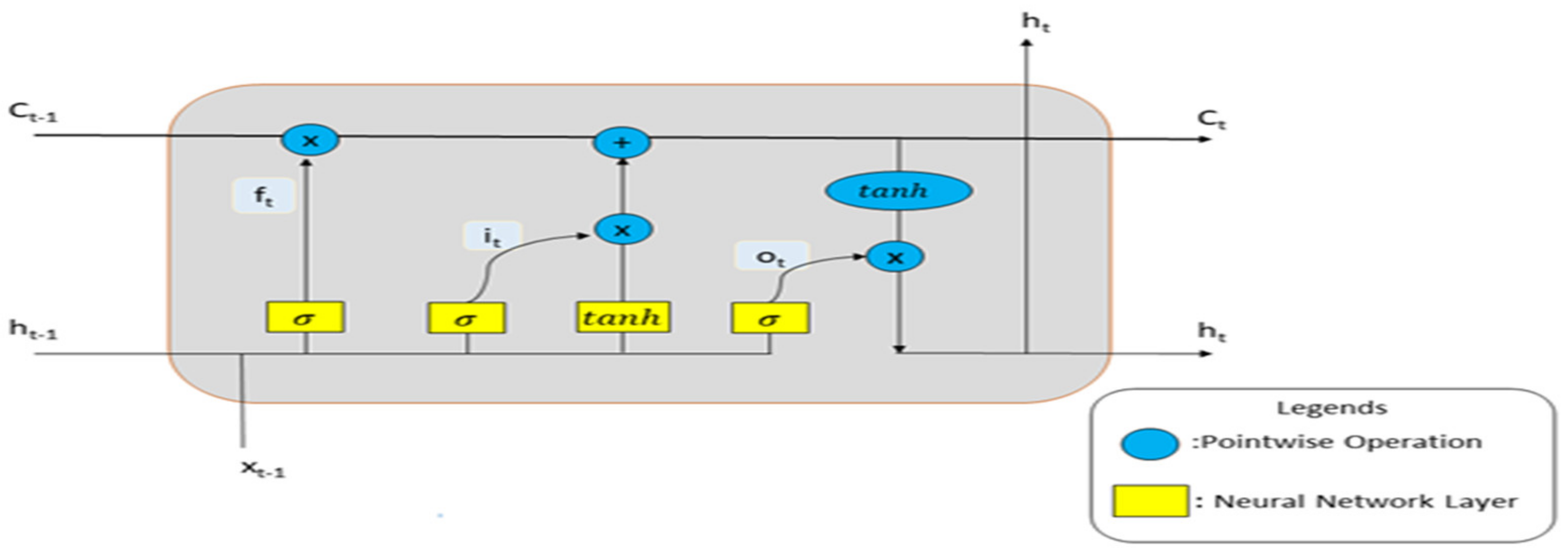There is a fresh approach to this problem proposed by [40]. Long Short-Term Memory is an RNN extension. Essentially, it is an RNN variant capable of learning about long-term associations. An LSTM representation is shown in Figure 1.

In the case of LSTMs, the problem of long-term dependency is purposely avoided. Long-term memory is a natural state of things for them, and they do not have to exert any efforts to maintain it. In addition, as seen in Figure 1, LSTM introduces a new parameter c_t, which denotes the memory cell and is utilized to encode information up to the time t. The activity of a memory cell is governed by three gates: f_t, i_t, and it, which are referred to as the input gate, forget gate, and output gate, respectively, in the circuit diagram. The equations for the three gates are as follows.

$$f_t=\mathrm{sigmoid}\left(V_f{h}_{t-1}+U_f{x}_t+b_f\right),$$

(1)

$$i_t=\mathrm{sigmoid}\left(V_i{h}_{t-1}+U_i{x}_t+b_i\right),$$

(2)

$$o_t=\mathrm{sigmoid}\left(V_o{h}_{t-1}+U_o{x}_t+b_o\right).$$

(3)

The rest of the updating equations are as follows.

$$h_t=o_t\ast \tanh \left(c_t\right),$$

(4)

$$c_t=f_t\ast c_{t-1}+i_t\ast d_t,$$

(5)

Component-wise multiplication is denoted by *. To add information to the cell, the input gate adds it, the forget gate removes it, and the output gate chooses information from the cell to be utilized as input in the prior step. The first forget gate acquires information at epoch t as a function of the input x_t and the previous hidden layer h_t−1. If the forget gate’s value is close to one, the last memory cell c_t−1 will be retained. Otherwise, the data are deleted. Second, the new information is combined with the old concealed state to generate the input gate $i_t$. It is turned into a memory cell to create a new $c_t$. Finally, the output gate determines which information will be utilized to create the next concealed state. More information on the algorithm’s architecture may be found in [41].

GRU is also presented as a solution for the vanishing gradient issue, similarly to how LSTM works. Sherstinsky [42] presented an extension to the LSTM. The system’s recurrent units can handle long-term dependencies across a broad range of periods. In the GRU algorithm, the input and forgotten gates of the LSTM are coupled with a single update gate, which serves as both the input and forgotten gates. Furthermore, the cell states and the hidden states are combined in the method developed by [43]. The representation of a GRU cell can be seen in Figure 2.

The architecture has been enhanced by the addition of two additional gates. The two sorts of gates are reset gates and update gates. The gates are used to store information and transfer it ahead as needed. The following is the model for GRU that may be written utilizing the new gates.

$$r_t=\mathrm{sigmoid}\left(U_r{h}_{t-1}\ast x_t\right),$$

(6)

$$z_t=\mathrm{sigmoid}\left(U_z{h}_{t-1}\ast x_t\right),$$

(7)

$${\tilde{h}}_t=\tanh \left(U_t{r}_t{h}_{t-1}\ast x_t\right)$$

(8)

$$h_t=\left(1-z_t\right)h_{t-1}+z_t{h}_t$$

(9)

GRU’s performance is boosted by the reset and the update, which also saves time [44]. It is up to the reset gate and hidden layer to decide whether or not the knowledge gleaned from the prior state will be lost. Data parsing has had a significant impact on the model’s overall performance and speed. Please refer to [42] for further in-depth details.

CNN are specific types of networks that function very well when dealing with data that possess a grid-type architecture, such as time-series data, images, and streaming videos. The mathematical process that gave origin to the network’s name is referred to as “convolution.” CNN performs convolution. Then, pooling, normalizing, and completely connected layers follow, each with the main purpose of multiplication, dot product, or ReLU. The first layer in CNN is the convolutional layer. Convolutional layers convolve the input and transmit the output to the next layer. This is analogous to a neuron’s reaction to a particular stimulus in the visual cortex. Each convolutional neuron only processes information for its receptive field. Although fully linked feedforward neural networks may be used to learn features and categorize data, they are often unfeasible for bigger inputs such as high-resolution photos. The second layer is the pooling layer. Pooling layers reduce the size of data by combining the outputs of neuron clusters at one layer into a single neuron at the next layer. This makes the data smaller. Local pooling brings together small groups of people. Global pooling affects all the neurons in the feature map, which means it affects all of them. Two types of pooling are used a lot: max and average. In the feature map, max-pooling takes the maximum value from each cluster of neurons. Average pooling only takes the average value from each cluster. The third layer is the flattening layer. It consists of taking the pooled feature map that was created during the pooling stage and converting it into a one-dimensional vector using a one-dimensional vector transform. This is performed in order to be able to feed them as inputs to the thick layer later on. The last layer is the fully connected layer. When all neurons in one layer are connected to all neurons in another layer, they work together to make sense of things. A multilayer perceptron neural network is the same as one that has a lot of different layers. To classify images, the flattened matrix proceeds through a layer that is fully connected. Figure 3 represents a CNN.

The majority of the time, this form of network is employed in image processing. Images are seen as a two-dimensional grid of pixels by the system. When applied to time-series data, this method is highly successful. As a result, it regards time-series data as a one-dimensional space of space intervals. For a more in-depth study of CNN, we recommend the book [45].

4. Data and Analysis

The dataset of this study is obtained from the publicly available website [46]. The data set contains the total electricity production of Turkey and is measured in MWh. It aggregates the electricity production from natural gas, lignite, river, import coal, wind, solar, fuel oil, geothermal, asphaltite coal, black coal, biomass, naphtha, LNG, import, and waste heat. The data set represents the real-time production of Turkey. We obtained the daily total electricity loads of Turkey for the periods between 5 January 2015, and 26 December 2021. The data set starts on Monday and ends on Saturday. The data set contains 2548 observations that correspond to 364 weeks. The electrical demands for all days in the forthcoming week are projected based on measurements from which complete weeks of lags are included in the prediction. We use the sliding window technique to forecast one to seven days ahead of observations. In each case, different lag lengths and numbers of nodes are used. The analysis is perfombed by using Python libraries Keras and Sklearn on the compiler Atom. 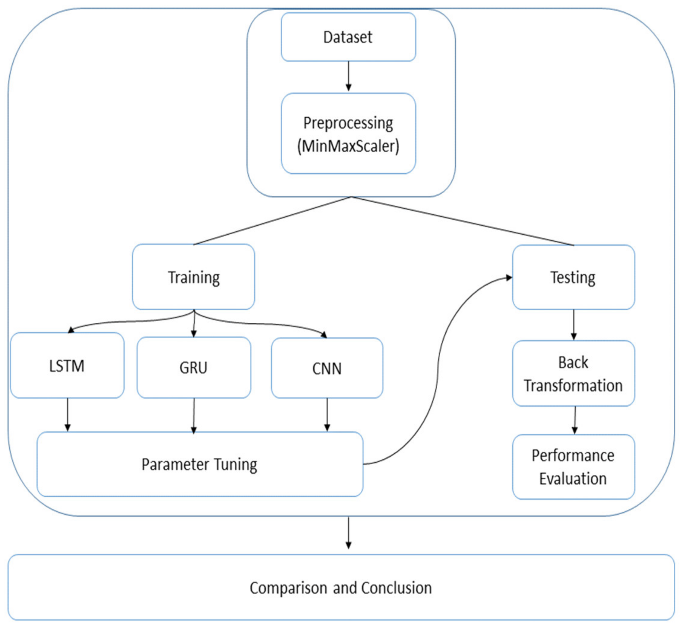Figure 4 summarizes the analysis procedure of the manuscript.

Our methodology consists of five steps as Figure 4 indicates, and these steps are summarized as follows:

• Since high valued values may yield high weight values, high weight values are often unstable, resulting in poor learning performance and input sensitivity, which leads to greater generalization error. To overcome instability, the entire data set is transformed by using min–max scaler transformation:

  $$X_n=\frac{X-X_{min}}{X_{max}-X_{min}},$$

  (10)

  where $X$ represents the observation, and $X_{min}$ and $X_{max}$ represent the lowest and highest values of the data set, respectively. After the transformation, the data set is divided into train and test sets. In the train set, the hyper parameter of the algorithm is decided, and on the test set, the algorithm runs on observations that are not used in training the data. The train set contains 312 weeks of observations while the test set contains 52 weeks of observation. The first six years act as the training data while the last year serves as the test set. Approximately, the training set contains 85% of the data while the test set contains 15%.
• In the second step, LSTM, GRU, and CNN algorithms are trained on the training set. A different number of lag lengths (sliding window length) and the number of nodes were tested to achieve the highest performance. The sliding window lengths are as follows: 1 week, 2 weeks, 3 weeks, 4 weeks, half a year, a year, one and a half year, and two years. Because the proposed deep learning design is data-driven, it is not possible to talk about a separate architecture. As a consequence, different numbers of nodes are chosen to find the best structure because the number of nodes that is employed is determined by the size of the inputs. For each sliding window, we employed a total of 100 nodes. In each model, Adam was used as the optimizer, and the mean square error was used as the loss function.
• In the third step, the lag lengths and number of nodes with the highest performance are run on the test set.
• In the fourth step, forecasted values are back-transformed to the observed range.
• In the last step, performance metrics are calculated to compare the performances of the algorithms. Three different performance metrics are utilized. These are mean absolute error (MAE), root mean squared error (RMSE), and coefficient of determination (R²). The formulas for each metric are given as follows:

  $$R^2=1-\frac{S{S}_{res}}{S{S}_{tot}},$$

  (11)

  $$RMSE=\sqrt{MSE}=\sqrt{\frac{1}{n}{\displaystyle \sum _{i=1}^n}{\left(y_i-{\widehat{f}}_i\right)}^2}=\sqrt{\frac{1}{n}{\displaystyle \sum _{i=1}^n}{e}_i{}^2}$$

  (12)

  $$MAE=\frac{1}{n}{\displaystyle \sum _{i=1}^n}\left|y_i-{\widehat{f}}_i\right|=\frac{1}{n}{\displaystyle \sum _{i=1}^n}\left|e_i\right|,$$

  (13)

  where $S{S}_{res}={\displaystyle \sum _{i=1}^n}{\left(y_i-\widehat{f_i}\right)}^2={\displaystyle \sum _{i=1}^n}{e}_i{}^2$; it is known as the residual sum of squares and $\widehat{f_i}$ is the anticipated output. $S{S}_{tot}={\displaystyle \sum _{i=1}^n}{\left(y_i-\overline{y}\right)}^2$ is the total sum of the square, and $\overline{y}$ is the mean of the observed data. Small values of RMSE and MAE indicate good performance while a value near 1 for $R^2$ represents a good fit.

The computer’s operating system is Windows 10, with a CPU Intel(R) Core(TM) i7-10510U and 8 GB of RAM, on which the algorithms are trained. We used the Keras library with an Adam optimizer with a learning rate of 0.001 and an epoch size of 100 to train the models mentioned above. An early stop mechanism is also employed to obtain the best possible outcome on the test set. MSE is used as the loss function while the activation function is set as ReLU. In LSTM, the following layers are utilized: LSTM layer with shape of (1,100) while the dense layer shape has shape (1,7). The computation time of LSTM is 3 s for each step. We employed a fixed window size for CNN layers. Columns are assigned to features, while rows are assigned to lagged values. The computation time is 2 s for each step. The architecture of the CNN is convolution layer of size (None, 1,64), MaxPooling layer of size (None, 1,64), flatten layer of size (None, 64), dense layer (None, 100), and dense layer (None, 7). Finally, the computation time for GRU is 3 s for each step. GRU consists of GRU layer of size (1,100) and dense layer of (1,7). The performance metrics for LSTM for different lag lengths on the test set are given in

Table 3. Performance metrics of LSTM on train set for different lag size.

Estimated Values
	${\widehat{\mathit{y}}}_{\mathit{t}}$	${\widehat{\mathit{y}}}_{\mathit{t}+1}$	${\widehat{\mathit{y}}}_{\mathit{t}+2}$	${\widehat{\mathit{y}}}_{\mathit{t}+3}$	${\widehat{\mathit{y}}}_{\mathit{t}+4}$	${\widehat{\mathit{y}}}_{\mathit{t}+5}$	${\widehat{\mathit{y}}}_{\mathit{t}+6}$
Panel A: Lag length = 7
MAE	15,699.05	24,122.23	29,272.79	32,555.04	34,794.46	36,880.26	38,159.13
RMSE	24,521.72	38,779.39	45,610.30	50,527.04	53,893.34	56,125.76	57,531.93
R2	0.92	0.80	0.73	0.67	0.62	0.59	0.57
Panel B: Lag length = 14
MAE	15,581.20	22,976.76	27.896.99	31,732.34	34,604.03	36,783.64	37,949.07
RMSE	23,701.21	36,435.10	44,048.82	50,052.43	54,024.80	56,539.06	5793.76
R2	0.93	0.83	0.75	0.67	0.62	0.59	0.56
Panel C: Lag length = 21
MAE	19,410.90	29,598.37	36,034.68	40,335.45	41,303.46	43,352.67	43,856.13
RMSE	31,150.22	47,841.76	60,509.59	68,103.54	68,850.81	65,431.78	63,913.05
R2	0.87	0.70	0.52	0.40	0.39	0.45	0.47
Panel D: Lag length = 28
MAE	17,153.52	26,952.24	32,011.75	35,466.31	38,208.38	38,528.40	39,586.90
RMSE	26,279.81	40,563.74	48,472.51	53,813.52	57,249.44	58,689.03	59,796.33
R2	0.91	0.79	0.69	0.62	0.57	0.55	0.54
Panel E: Lag length = 182
MAE	17,451.31	25,541.31	28,991.61	31,138.22	32,718.46	33,835.26	36,008.39
RMSE	2509.98	38182.16	43,601.38	47,018.59	48,844.44	49,449.23	51,886.17
R2	0.92	0.81	0.75	0.71	0.69	0.68	0.65
Panel F: Lag length = 364
MAE	15,502.61	23,570.24	27,577.30	30,641.93	32,041.78	32,760.72	34,045.72
RMSE	21,561.57	32,538.21	37,346.16	40,974.10	42,506.322	43,478.06	45,782.79
R2	0.94	0.86	0.82	0.78	0.77	0.76	0.73
Panel G: Lag length = 546
MAE	16,262.13	24,255.68	30,396.81	32,241.56	32,610.89	35,494.71	36,846.01
RMSE	22,835.58	33,540.96	40,476.96	43,986.36	45,137.09	47,090.86	48,918.94
R2	0.93	0.85	0.79	0.75	0.74	0.71	0.69
Panel H: Lag Length = 728
MAE	16,976.59	24,364.76	28,113.48	31,015.43	34,180.15	36,634.84	38,668.64
RMSE	23,308.74	33,971.50	39,104.11	42,854.71	46,421.85	49,947.78	52,931.25
R2	0.93	0.85	0.80	0.76	0.72	0.68	0.64

.

Here, $\widehat{y_t}$ represents the next-day forecast, ${\widehat{y}}_{t+1}$ represents the two-day-ahead forecast, and in the same manner, ${\widehat{y}}_{t+6}$ represents the seven days ahead forecast. Each panel represents the performance metrics when different lag lengths are used. For example, if we consider Panel A, we may summarize the forecasting procedure as $x_{t-7};x_{t-6}\dots ,x_{t-1}$ are used to forecast ${\widehat{y}}_t\widehat{ },{\widehat{y}}_{t+1}\dots ,{\widehat{y}}_{t+6}$ where $x_t$ represents the input values.

According to the results given in Table 3, the best performance is achieved when lag length is determined as 364. This case is given in Panel F. R² for the day ahead forecast is calculated as 0.94, and it decreased to 0.73 for seven days ahead forecasts. Moreover, in this case, the algorithm achieves its lowest MAE and RMSE for each forecasted value.

Table 4. Performance metrics of GRU on train set for different lag size.

Estimated Values
	${\widehat{\mathit{y}}}_{\mathit{t}}$	${\widehat{\mathit{y}}}_{\mathit{t}+1}$	${\widehat{\mathit{y}}}_{\mathit{t}+2}$	${\widehat{\mathit{y}}}_{\mathit{t}+3}$	${\widehat{\mathit{y}}}_{\mathit{t}+4}$	${\widehat{\mathit{y}}}_{\mathit{t}+5}$	${\widehat{\mathit{y}}}_{\mathit{t}+6}$
Panel A: Lag length = 7
MAE	19,394.83	29,989.55	37,397.96	43,087.90	47,997.79	49,682.09	50,972.89
RMSE	29,685.12	44,974.25	54,601.31	60,463.16	64,933.41	67,078.77	68,605.49
R2	0.88	0.73	0.61	0.52	0.45	0.42	0.39
Panel B: Lag length = 14
MAE	18,442.08	30,479.90	39,077.06	47,732.60	50,860.67	51,966.74	51,205.42
RMSE	26,251.80	44,369.63	57,378.43	67,591.32	71,879.19	73,737.69	73,698.62
R2	0.91	0.74	0.57	0.41	0.33	0.30	0.29
Panel C: Lag length = 21
MAE	19,200.65	31,087.74	40,138.71	47,851.97	54,597.72	57,569.05	58,608.46
RMSE	27,639.07	43,832.20	54,643.56	64,115.14	72,562.20	77,055.52	78,916.40
R2	0.90	0.75	0.61	0.46	0.32	0.23	0.19
Panel D: Lag length = 28
MAE	18,268.73	30,688.07	39,384.86	47,825.35	55,541.09	60,740.50	66,4387.58
RMSE	25,493.66	43,038.88	55,662.88	65,935.28	74,158.95	78,728.52	83,011.19
R2	0.91	0.76	0.60	0.43	0.29	0.20	0.10
Panel E: Lag length = 182
MAE	20,759.19	30,960.13	30,643.27	32,815.74	36,172.25	37,763.67	40,939.88
RMSE	28,232.99	42,474.98	44,552.46	47,638.76	49,405.75	48,905.59	52,472.01
R2	0.90	0.76	0.74	0.70	0.68	0.69	0.64
Panel F: Lag length = 364
MAE	20,281.40	30,132.46	38,391.27	37,534.92	3866.23	40,951.27	44,929.31
RMSE	26,900.16	39,285.18	48,824.45	48,195.70	51,052.09	52,933.20	56,855.68
R2	0.91	0.80	0.69	0.69	0.66	0.64	0.58
Panel G: Lag length = 546
MAE	22,134.43	34,811.60	45,676.56	52,662.06	49,250.80	48,575.73	46,582.51
RMSE	28,952.59	44,469.78	57,428.50	66,416.10	64,495.22	64,762.98	63,057.94
R2	0.89	0.74	0.57	0.46	0.46	0.46	0.48
Panel H: Lag Length = 728
MAE	19,724.99	39,265.06	49,729.89	49,852.41	52,810.00	45,557.80	64,353.77
RMSE	27,133.75	50,171.98	61,195.24	61,860.46	64,526.60	57,388.58	81,414.38
R2	0.90	0.67	0.51	0.50	0.46	0.57	0.14

represents the performance metrics of GRU on the test set.

According to the results given in Table 4, the best performance is achieved when lag length is determined as 364. The case is given in Panel F. The R² for the day ahead forecast is calculated as 0.91, and it decreased to 0.58 for seven days ahead forecasts. Moreover, in this case, the algorithm achieves its lowest MAE and RMSE for each forecasted value. Table 4 represents the performance metrics of GRU. The difference between GRU and LSTM occurs in the mid-term forecast. As both tables indicate the performance of LSTM is better than GRU. The R² of GRU in the mid-term decreases faster than in the LSTM case. Lastly,

Table 5. Performance metrics of CNN on train set for different lag size.

Estimated Values
	${\widehat{\mathit{y}}}_{\mathit{t}}$	${\widehat{\mathit{y}}}_{\mathit{t}+1}$	${\widehat{\mathit{y}}}_{\mathit{t}+2}$	${\widehat{\mathit{y}}}_{\mathit{t}+3}$	${\widehat{\mathit{y}}}_{\mathit{t}+4}$	${\widehat{\mathit{y}}}_{\mathit{t}+5}$	${\widehat{\mathit{y}}}_{\mathit{t}+6}$
Panel A: Lag length = 7
MAE	16,356.06	25,708.07	31,697.22	35,591.24	37,120.37	37,861.61	39,063.72
RMSE	25,765.27	40,912.00	49,607.64	55,626.94	58,202.84	58,216.24	59,015.31
R2	0.91	0.78	0.68	0.60	0.56	0.56	0.55
Panel B: Lag length = 14
MAE	16,445.03	24,700.00	30,280.47	35,430.57	37,406.25	38,861.45	37,997.71
RMSE	25,034.40	39,139.99	48980.26	55,134.06	57,333.28	59,121.08	58,697.51
R2	0.92	0.80	0.69	0.60	0.57	0.55	0.55
Panel C: Lag length = 21
MAE	16,724.63	26,348.3	32,906.18	37,370.37	38,553.61	38,771.68	39,881.52
RMSE	2622.37	40,865.14	50,672.01	56,788.21	58,362.08	57,924.47	59,204.25
R2	0.91	0.78	0.66	0.58	0.56	0.57	0.54
Panel D: Lag length = 28
MAE	18,348.50	27,976.51	33,386.07	37,748.13	41,008.70	40,982.05	40,650.68
RMSE	26,852.14	41,811.17	51,001.62	58,105.20	61,217.19	60,627.58	60,271.08
R2	0.90	0.77	0.66	0.56	0.51	0.52	0.52
Panel E: Lag length = 182
MAE	21,458.65	29,987.71	32,860.28	37,032.26	41,267.43	39,066.82	39,647.72
RMSE	31,305.85	44,841.78	48,393.33	54,752.09	59,953.79	57,048.44	57,289.49
R2	0.87	0.74	0.69	0.61	0.53	0.58	0.57
Panel F: Lag length = 364
MAE	19,893.01	28,803.52	34,274.11	37,084.61	39,495.88	37,885.74	36,249.55
RMSE	29,312.52	40,326.48	47,292.92	50,441.64	54,319.91	52,452.09	50,747.24
R2	0.89	0.79	0.71	0.67	0.61	0.64	0.66
Panel G: Lag length = 546
MAE	17,694.61	27,589.23	33,409.78	37,503.49	38,201.54	39,553.46	37,239.67
RMSE	25,212.95	39,388.38	46,514.93	52,304.83	52,018.61	53,394.24	52,067.60
R2	0.92	0.80	0.72	0.64	0.65	0.63	0.65
Panel H: Lag Length = 728
MAE	17,505.89	27,472.71	29,315.02	32,728.29	35,896.08	35,859.17	34,807.66
RMSE	24,884.32	38,493.64	41,143.23	46,708.97	50,173.87	50,275.14	49,692.07
R2	0.92	0.81	0.78	0.72	0.67	0.67	0.67

represents the performance metrics of CNN.

In this case, according to the performance metrics, the best length is 546, which represents a year and a half. R² for the next day forecast is calculated as 0.92, while for seven days ahead, it is calculated as 0.66. As in the case of GRU, R² decreases as the length of the forecasting horizon increases. When CNN is compared to LSTM and GRU, it has the second-best performance according to the calculated performance metrics.

5. Discussion

The aim of this study is to forecast short-term to mid-term electrical usage utilizing deep learning algorithms such as LSTM, GRU, and CNN. These algorithms were selected for this investigation because they have been utilized effectively in various time-series studies. Moreover, the proposed models can handle entire data sequences as well as single data points. Although there are many powerful RNN algorithms, in this study, we employed LSTM because the LSTM cell increases long-term memory capacity in an even more efficient manner since it allows learning even more parameters. Moreover, it has the capacity of handling a large amount of non-linear data [47]. This makes it the most effective method of forecasting, particularly when there is a longer-term trend in the data set. We trained LSTM and others algorithms in the same way that we would estimate a time series model of Box–Jenkins. Algorithms, as a time series model, use the lags of the time series data that we are analyzing. The suggested methodology exclusively employs data derived solely from time-series itself. As a result, it is effective, straightforward, and forceful. The univariate structure of the methodology leads it to be utilized globally as well as locally

It should also be noted that we represented the loads in a univariate manner; thus, the information is entirely generated from the data itself, which increases the model’s efficacy while minimizing its overall complexity. To the best of our knowledge, this is the first research study that compares Turkey’s short-term and mid-term algorithms. Because of this, the suggested model is not limited to the Turkish market but may also be applied in any other market. It does not need the use of any exogenous variables or other information. It is worth mentioning that this is the first research to use deep learning algorithms to simulate the short-term Turkish power market.

Table 6. Summary of the performance metrics of the investigated models on train set.

Estimated Values
	${\widehat{\mathit{y}}}_{\mathit{t}}$	${\widehat{\mathit{y}}}_{\mathit{t}+1}$	${\widehat{\mathit{y}}}_{\mathit{t}+2}$	${\widehat{\mathit{y}}}_{\mathit{t}+3}$	${\widehat{\mathit{y}}}_{\mathit{t}+4}$	${\widehat{\mathit{y}}}_{\mathit{t}+5}$	${\widehat{\mathit{y}}}_{\mathit{t}+6}$
Panel A: LSTM (Lag Length = 364)
MAE	15,502.61	23,570.24	27,577.30	30,641.93	32,041.78	32,760.72	34,045.72
RMSE	21,561.57	32,538.21	37,346.16	40,974.10	42,506.322	43,478.06	45,782.79
R2	0.94	0.86	0.82	0.78	0.77	0.76	0.73
Panel B: GRU (Lag length = 364)
MAE	20,281.40	30,132.46	38,391.27	37,534.92	3866.23	40,951.27	44,929.31
RMSE	26,900.16	39,285.18	48,824.45	48,195.70	51,052.09	52,933.20	56,855.68
R2	0.91	0.80	0.69	0.69	0.66	0.64	0.58
Panel C: CNN (Lag length = 546)
MAE	17,694.61	27,589.23	33,409.78	37,503.49	38,201.54	39,553.46	37,239.67
RMSE	25,212.95	39,388.38	46,514.93	52,304.83	52,018.61	53,394.24	52,067.60
R2	0.92	0.80	0.72	0.64	0.65	0.63	0.65

summarizes the performance metrics of the proposed model for the best cases of each.

LSTM and GRU had the best performance when lag lengths are set as 364 while the best performance of CNN is achieved with 546 lag lengths. According to the empirical results provided in Table 6, the best algorithm when compared to CNN and GRU is found to be LSTM. It has an R² of 0.94 in the short-term and 0.73 in the mid-term. Moreover, it is interesting to see that GRU and CNN have high R² in the short-term forecasting but decrease gradually in mid-term forecasts. Thus, LSTM with a one-year lag can be used efficiently to model and forecast the daily Turkish electricity load of Turkey. The proposed model only needs its own lagged values; when compared to the other studied in the literature, it is more efficient and powerful. In some cases, we obtained very good forecasting results without using any exogenous variables such as temperature, precipitation, and other influencing factors.

The power of the proposed model not only comes from its univariate case but it can also handle multi-step forecasting with low computation costs. There are many valuable studies that attempt to forecast electricity loads of Turkey or stations located at Turkey. The next two paragraphs compare the results of our study with the literature on Turkish case, which uses ML, DL, or Fuzzy time series analyses. The first paragraph devoted to multivariate case, while the last paragraph is about the univariate case.

In their studies, Tosun et al. [33] proposed to forecast short-term electricity loads of Düzce, Turkey with ANN. The model used hour, temperature, previous temperature, and previous consumption as the features. The proposed model is a multivariate methodology, and the results showed that, on average, the best R² for hourly electricity consumption ranged in 0.927 and 0.978. Bozkurt et al. [32] also preferred multivariate modeling for short-term electricity loads. The feature set of ANN contains calendar date, previous load estimation plan, electricity price, weather, and currency. Each feature set also contains a different number of features. The total number of features to train ANN was 19. The performance metrics of MAPE ranged from 0.98 to 3.26. Luy et al. [36] used temperature as a feature of the proposed algorithms to forecast short-term electricity loads of Turkey. The other features are the last day of consumption, the last week of consumption, the weekly load trend, and the weekly air temperature trends. In the best case, MAPE is calculated as 3.389. Kaytez [37] used multivariate methodology to forecast net electricity consumption of Turkey and MAPE of the best case ranging from 0.971 to 1445. Several environmental variables are used by [1] to forecast loads of Turkey in short- and mid-term periods. In the best case, the performance metric of R² is calculated at 0.907.

Hamzaçebi et al. [35] used ANN in a univariate case to forecast monthly electricity loads of Turkey. Different ANN combinations are compared, and the best model had RMSE ranged from 438 to 572.95.

In light of the above two paragraphs, our study is as powerful as the multivariate cases according to Table 6. Moreover, we introduced a model in the univariate case that can be used in both short- and mid-term forecasting. To the best of our understanding, there is only one univariate time series methodology that utilizes ANN to forecast monthly electricity loads of Turkey. We would like to emphasize once again that the proposed model is based on a univariate case and is capable of forecasting daily electricity loads of Turkey in multiple steps. Thus, it can be used to forecast and model Turkish electricity loads to have better projections and planning.

6. Conclusions

Electricity is a critical indicator of human life and the health of a country’s economic structure. When developing economic planning, it is vital to have precise projections of power consumption levels. Accurate energy demand forecasting is crucial for decision-makers and power-generating firms when it comes to policy creation and power generation planning. Several approaches have been explored in the past to increase peak load forecasting accuracy. The data set used in this study is a daily data collection used to assess electrical demands. In classical time series analysis, despite the fact that the methodology’s predicting ability has been shown, some assumptions must be satisfied, such as the assumption of stationarity. It should be emphasized that the Box–Jenkins type models are linear time series models, as opposed to the other types of deep learning and machine learning algorithms. In the literature, there are many valuable works that compare ARIMA-type models with the others. For example, Akdi et al. [2] showed that HR is more powerful than AR or Tokgöz, and Ünal [48] compared ARIMA with deep neural networks and showed that ARIMA had the lowest MAPE. Instead of using the Box–Jenkins approach, we used a very customized model of deep learning in our study. The proposed model has no assumptions, such as the stationarity of the investigated model or the residuals terms of the model that should be normally distributed and are uncorrelated. This feature can be shown as the strength of the proposed model.

Although the suggested model’s primary strength is its univariate structure, further research into the relationships between electrical demand and meteorological parameters, such as those described in [1], will be possible via the use of deep learning algorithms. Additionally, as mentioned in [49], the combination of time series approaches and deep learning algorithms to forecast electricity consumption may be of interest; on the other hand, as in [47], the effects of wavelet transformation can be investigated. To anticipate power demands in Turkey, it is also possible to study the hybrid approaches of [5] and the machine learning methods of [50], which may be used in both uni- and multivariate contexts. Moreover, the proposed models are utilized and investigated as standalone. It is also possible to use them together as hybrid models or in an ensemble manner as in [51]. Since there is no exact rule to decide the hyper parameters of the proposed algorithm. This can be shown as the weakness of the models and the optimization of the proposed algorithms can be performed by using the metaheuristic algorithms of [52]. We leave these ideas as future research opportunities.

Weather and seasonal impacts have a direct influence not only on load demand but also on the utilization of certain renewable energy sources in Turkey’s power grid; hence, the load forest must be considered as a collection of factors including people’s daily routines [53]. It may also be interesting to investigate the influence of weather-related time series and people’s daily habits on power demand forecasting as a challenge. The holiday weekdays and weekends affect power use in diverse ways, as has been shown in several research studies [54]. It is obvious that the forecasting ability of the models will be improved by including these elements as the features of the algorithms. In addition, the impact of these variables on the forecasting capacity of the model should be investigated with different data pre-processing techniques [55].

In this study, the main aim was to train and test different deep neural networks to forecast short-term to mid-term forecasting of Turkish electricity load in a univariate sense. The proposed models are investigated to forecast 1 to 7 data points simultaneously and it was observed that, overall, LSTM has the best performance compared to CNN and GRU. Long-term forecasting is more challenging than short- and mid-term forecasting. There are three categories of issues in long-term power demand forecasting: what technical and economic aspects to include, what regional and temporal scales to pick, and to what degree long-term and short-term uncertainty should be taken into consideration [12]. It might be more challenging to model long-term electricity loads by univariate time series methodologies. The other influencing variables should be considered in this task.

The development of effective energy forecasting models is critical in the development of energy policy, which may involve planning, production, pricing, and consumption. As illustrated in this research study, determining the appropriate lag length and plugging in models improve the accuracy of forecasts and predictions. In conclusion, LSTM should be viewed as a potent tool for electrical load forecasting in the short- and mid-term for both short- and mid-term forecasting. Because this model more closely matches the data than GRU and CNN models, it will be more helpful in developing policies based on energy demand. In this context, the findings of this study’s methodology provide valuable evidence for policymakers on how to interfere in electricity markets in a manner that legitimizes evidence-based policymaking, which is critical in today’s world.