A Transfer Learning Approach for Lumbar Spine Disc State Classification

Abstract

Recently, deep learning algorithms have become one of the most popular methods and forms of algorithms used in the medical imaging analysis process. Deep learning tools provide accuracy and speed in the process of diagnosing and classifying lumbar spine problems. Disk herniation and spinal stenosis are two of the most common lower back diseases. The process of diagnosing pain in the lower back can be considered costly in terms of time and available expertise. In this paper, we used multiple approaches to overcome the problem of lack of training data in disc state classification and to enhance the performance of disc state classification tasks. To achieve this goal, transfer learning from different datasets and a proposed region of interest (ROI) technique were implemented. It has been demonstrated that using transfer learning from the same domain as the target dataset may increase performance dramatically. Applying the ROI method improved the disc state classification results in VGG19 2%, ResNet50 16%, MobileNetV2 5%, and VGG16 2%. The results improved VGG16 4% and in VGG19 6%, compared with the transfer from ImageNet. Moreover, it has been stated that the closer the data to be classified is to the data that the system trained on, the better the achieved results will be.

1. Introduction

Since the 1970s, researchers have built systems to analyze medical images and diagnose diseases based on images uploaded to computers. The reason for the spread of medical images and the interest of researchers in this analysis is due to a large number of diseases and their spread in the world, especially lower back diseases. The causes of this pain can be due to spinal deformity, herniated disc, osteoporosis, or muscle strain as a result of modern lifestyle through office work. In addition, sitting for long hours in front of computers has led to an increase in the spread of lower back pain (LBP) [1,2].

LBP is considered the main cause of lost productivity due to disability, and its percentage increases among the elderly [3,4]. Neuritis that is due to either mechanical pressure or chemical irritation leads to pain [5]. In addition, spinal stenosis and disc herniation are significant factors in LBP [6]. The lumbar spine consists of five vertebrae, labeled L1 to L5, and these vertebrae progressively increase in size moving downward. Each vertebra is connected with the other vertebrae by intervertebral discs. The intervertebral discs help stabilize the spine and act as shock absorbers, in addition to protecting the bones from friction and interference. These discs are filled with a gel-like fluid and, if they dry out, it is an indication of some problem [7].

Disc herniation and spinal stenosis are two of the most common lower back diseases. The process of diagnosing pain in the lower back is performed by radiologists and doctors analyzing medical images. Due to the number of these images and the analysis process, which requires expertise in the field of diagnosis, as well as the potential fatigue of experts, the difference of opinion among doctors, and the financial cost of this process, researchers are moving toward building computer systems that help experts to make decisions and speed up the diagnosis process. There are many types of medical imaging techniques that help radiologists in making decisions. The most common of these techniques are computed tomography (CT), X-ray, magnetic resonance imaging (MRI), and thermal images. MRI is the most popular technique used to diagnose spinal diseases [8,9,10,11,12,13].

The processes of computer-assisted diagnostics and medical imaging analysis mainly rely on machine learning (ML). After the development of ML techniques and the emergence of the field of deep learning (DL), DL has been adopted as one of the adopted methods in the diagnostic process. Although there are many ML techniques to analyze medical images in various fields, DL has become the state-of-the-art method to analyze and diagnose medical problems due to its accuracy. Currently, deep learning on MRI images has become the approved method for many researchers, including for lumbar spine diagnosis [14].

In the medical image analysis process, Convolutional Neural Network (CNN) is currently one of the best deep learning algorithms. In CNN, the spatial relationships are preserved after filtering the input images. In the field of radiology, these relationships are very important [15,16,17]. Features in CNN can be extracted automatically. The final prediction can be made based on the features that were extracted from the input image combined with layers in CNN; weight factors change over the training procedure [18].

It is known that CNN models require large amounts of data for the purpose of training. The most important challenge facing these models is the lack of data for the purpose of training them. Collecting a large amount of labeled data, especially medical data, is very difficult. However, the problem of lack of data is solved by using transfer learning. The transfer method is considered efficient in solving the problem of lack of data. Simply, the model is trained on a large amount of labeled data, such as (ImageNet). In the next step, the model is fine-tuned for training on small labeled data [19,20,21,22].

This paper aims to solve the problem of lack of training data in disc state classification of the lumbar spine, improve the performance of disc state classification tasks and to determine if the kind of images used for transfer learning has an impact on performance. In this regard, we propose several procedures to overcome these challenges. The contributions of this work can be summarized as follows:

• The problem of a lack of training data has been solved by utilizing transfer learning.
• The novel selection method is applied to select the most essential images. This method saves us a lot of time and effort in selecting important images to be used in the process of classifying lumbar spine discs compared with the manual method. Where images are selected automatically and quickly, this method is applied to the images taken from the magnetic resonance devices to describe the problem of the lumbar spine.
• A custom grading system was built for radiologists to label images.
• We proposed a new technique to extract ROI that splits the images into many blocks, and we identified the most important blocks. The proposed ROI achieved excellent results when we applied it in disc state classification. In the process of diagnosing images of lumbar spine discs, there were many shapes in the image overlapping with the object to be analyzed, such as the image of the intervertebral disc.
• A new private lumbar spine dataset was built. This dataset had 1448 MRI images of the lumbar spine. We had 905 images belonging to the axial T2, 181 belonging to sagittal T2, and 362 belonging to myelography. In this dataset, we labeled two subjects in lumbar spine disc state and canal stenosis.
• Three datasets were built, two as sources and one as a target. One of them represented the final database, with label data on which the classification process was carried out. The second dataset (209,083 MRI images) described an unlabeled dataset that was used in the training process from scratch. Finally, the third dataset (16,441 MRI images) was a dataset compiled from several public datasets labeling brain tumors.
• Various training procedures have been performed with many deep learning models.
• It has been demonstrated that using TL from the same domain as the target dataset may increase performance dramatically.
• Applying the ROI method improved the disc state classification results in VGG192%, ResNet50 16%, MobileNetV2 5%, and VGG16 2%.
• The results improved in VGG16 4% and in VGG19 6% compared with those transferred from ImageNet. This is because labeled datasets and unlabeled dataset images are closer to lumbar spine MRI than the images in ImageNet.

This paper is organized as follows. Section 2 illustrates the work related to lumbar spine diseases and disc state classification. Section 3 presents the details of the datasets that are used in the experiments, the steps taken to build our dataset, and various procedures and methods applied to these datasets, which led to improving the classification task. Section 4 describes the results and performances of the models. Section 6 offers a conclusion of the work.

2. Related Work

Deep learning has become the trailblazing method for analyzing and diagnosing medical conditions because of its accuracy. There have been many previous studies on computer-aided techniques. Sa et al. [23] proposed a method of disc detection through X-ray images by using Faster R-CNN. Due to the lack of medical images, they fine-tuned a pre-trained deep network on a small medical dataset and obtained satisfactory results. The method achieved an average accuracy of 0.905, with an average computation time per image of three seconds.

Kuok et al. [24] proposed a hybrid approach using image processing for the detection of the vertebrae and CNN in the segmentation task of the vertebrae. They used a private dataset from the National Cheng Kung University Hospital in Taiwan for 60 X-ray images. The segmentation efficiency using the proposed method was significantly elevated with a DSC value of 0.941.

Some studies using CT images, such as that of Navab et al. [25], worked on CT scans where the proposed approach was the automatic detection and localization of vertebrae in volumetric CT. The location of each part was predicted by the contextual information in the image by using deep feed-forward neural networks. A public dataset of 224 arbitrary field-of-view CT scans of the pathological cases was used to evaluate the method. The detection rate was 96% and the total operating time was less than three seconds.

In contrast, Zaho et al. [26] proposed a technique to perform the localization and segmentation of the vertebra applied on CT imaging using transfer learning; 500 spine CT images were used from a SpineWeb public dataset. The results displayed that the proposed approach could indicate considerable properties of the spinal vertebrae as well as provide useful localization and segmentation performance.

Some studies using MRI images, such as that of Jamaludin et al. [27], proposed an approach to automatically predict radiological scores in spinal MRIs. They also determined diseases based on radiation scores. They worked on a two-fold approach: (i) architecture and training of CNN and (ii) the prediction of a heat-map of evidence hotspots for each score. The results show that the hotspots of pathology and radiological scores can be projected at an excellent level.

Davies et al. [28] proposed a method that uses magnetic resonance of the cervical and lumbar spine to classify disc degeneration. The goal of this method was to explore the association between histological grading and magnetic resonance of IVD degeneration in the lumbar spine and the cervical spine for patients undergoing diskectomy.

Heinrich and Oktay [29] presented a method for finding anatomical landmarks in spine MRI scans by using Vantage Point Hough Forests and multi-atlas fusion. The proposed method achieved Dice segmentation overlaps of almost 90%, sub-voxel localization accuracy of 0.61 mm, as well as a processing time of approximately ten minutes per scan.

Hetherington et al. [30] proposed a method of vertebral level labeling and identification without the use of an outer chase device. The suggested CNN successfully distinguished ultrasound images of the sacrum, intervertebral spaces, and vertebral bones, with a 20-fold cross-validation precision of 88 percent. A total of 17 of 20 test ultrasounds provided a wealthy recognition of all vertebral levels and processed a real-time speed of 40 frames per second.

Kim et al. [31] proposed a new deep learning network to divide intervertebral discs from MRI spine images. The traditional method (U-net) is known to work well for medical image segmentation. However, its performance in terms of segmentation details, such as boundaries, is limited by structural limitations of the maximum clustering layers. The proposed network achieved 54.62% compared with 44.16% for convolutional U-net.

In contrast, Zhou et al. [32] suggested a deep learning-based detection algorithm. The data hail from Hong Kong University’s Department of Orthopedics and Traumatology. The MRI dataset consisted of samples from various age groups and used 2739 unhealthy and 1318 healthy samples. To train the CNN to detect the lumbar spine, they worked on a similarity function, and the proposed method compared similarities between vertebrae using an earlier lumbar image instead of distinguishing vertebrae using annotated lumbar images. S1 was identified due to its unique shape, and a rough area around it was removed in order to look for L1–L5. The accuracy, precision, mean, and standard deviation (STD) of the results were calculated, and this detection algorithm had an accuracy of 98.6 percent and precision of 98.9 percent. The majority of the failed findings were due to misplaced S1 vertebrae or undetected L5 vertebrae.

Whitehead et al. [33] worked on spine segmentation by proposing a technique that was not model based. They proposed a technique established on a string of four pixel-wise division networks. They used a dataset from UCLA Radiology, and each network chunk MR imaged at several scales. The input to the network in the chain was fed by the output from the previous network. Each sequential network produced an increasingly filtered segmentation outcome by using both the original image and the output from the last network as input. In comparison to the U-net segmentation method, the proposed approach improved the segmentation task in the vertebrae and discs at the rate of 1.3% and 4.9%, respectively.

In addition, Hu et al. [34] used deep learning to distinguish patients with LBP from healthy persons in static standing. They used 44 chronic LBP and healthy individuals and the spine kinematics and pressure points were listed. The outcomes showed that deep neural networks could identify LBP persons with a precision of up to 97.2%. The study showed the classification task with precision and recall could be carried out by deep learning networks.

Lu et al. [35] worked to classify MRI lumbar spinal stenosis using CNN, the natural language processing used to extract the labels for different types and degrees of spinal stenosis from radiology diagnoses. They used U-net architecture for the segmentation of the lumbar spine vertebrae and localization of the disc level. Data from the Department of Radiology of Massachusetts General Hospital during the period from April 2016 to October 2017 was used. In the segmentation task of the vertebral body, the standard guaranteed that all lumbar intervertebral discs could be taken away with the algorithm. The pass rate for the test group according to these criteria was 94%.

Palkar and Mishra [36] proposed a method to generate a single image containing all the important features from MR and CT images of the lumbar spine by using CNN and wavelet-based fusion. First, using wavelets, both MR and CT images were analyzed into detail and approximation coefficients. Then, using a CNN framework, approximation coefficients were fused with the corresponding detail. Finally, the fused image was generated using inverse wavelet transform. A SpineWeb public dataset was used. Experimental results indicated that the proposed method had performed well when compared with conventional methods.

Mbarki et al. [37] studied identification of a herniated lumbar disc by working on MRI, using CNN, based on the VGG16 geometry. A special dataset was used from Sahloul University Hospital in Sousse, Tunisia. U-net was used with an axial view MRI to locate and detail the location of the herniated lumbar disc. The accuracy of the proposed model was 94%.

Won et al. [38] validated the utility of the computer-assisted spinal stenosis classification system by comparing agreements between experts trained in CNN classifications and a diagnostic agreement between two experts. For the detection process, they used Faster R-CNN, and for the classification process, they used VGG network. After the grading agreement was completed, the differences in the results between each expert and the trained models were not considerable, while the final agreement between the trained model and the expert was 74.9% and 77.9%, respectively.

Lakshminarayanan and Yuvaraj [39] proposed a method for analyzing and classifying spinal vertebrae images. After scanning the spinal vertebrae, the images were analyzed and classified into different disc types using the CNN ConvNet algorithm. In their proposed model, they showed the CNN system was better than the SVM system. However, the precision of the SVM was 90%, while the CNN was 96.9%. The results stated that the proposed method provided speed and accuracy compared with traditional algorithms.

Medical imaging is a significant tool for diagnosis. Computer-aided diagnosis is gaining popularity with advances in computer technology such as deep learning. However, medical pictures are created using specialized medical equipment, and their collection and labeling by professionals is an expensive process. As a result, gathering adequate training data is often costly and challenging. Most of the related work for disc state classification used CNN models. It is known that CNN models require large amounts of data for training. The most critical challenge facing these models is the lack of data to train them. Collecting a large amount of labeled data is very difficult, especially medical data. Transfer learning technology may be applied for medical imaging analysis. Pre-training a neural network on the source domain and then fine-tuning it based on examples from the destination domain is a typical transfer learning strategy.

3. Materials and Methods

In this section, we will illustrate the datasets and the procedures that we applied to these datasets. This section consists of five parts: building the lumbar spine dataset, analysis of collected dataset, the proposed ROI, the datasets used in this work, and the proposed methods.

3.1. Building the Lumbar Spine Dataset

Real world data often contain a lot of noise, errors, and missing values. This data may be in a format that is not directly usable in various applications such as ML. Therefore, pre-processing the data is an essential step to clean that data and convert it into a format suitable for use as required. In general, in the context of artificial intelligence, pre-processing aims to raise the quality of datasets to improve the accuracy and efficiency of different models and systems.

3.1.1. Raw Data Collection

Data collection is one of the significant obstacles to deep learning. The spread of deep learning and artificial intelligence applications has created many applications in which sufficiently classified data are not available, especially in which deep learning automatically engineers and creates features, unlike traditional machine learning. However, deep learning leads to the need for large amounts of classified data. One of the exciting things is that modern research has become focused on the process of collecting data and building databases in a considerable way in all fields.

The private dataset was collected for subjects with LBP in the lumbar spine for a period of one year, from 1 January 1 2020 to 1 January 2021, from the Fallujah Teaching Hospital—Radiology and Sonar Department.

3.1.2. Novel Selection Method

The PACK server has a large number of images; the main problem with these images is that they are raw data, unlabeled, and belong to many diseases. During a full year of work at the Fallujah Teaching Hospital, we collected 48,642 MRI images belonging to 400 patients suffering from lumbar spine problems. Radiologists in the hospital’s radiology department were able to label images for only 181 patients. So, for those 181 patients (mean age ± standard deviation, 44 years ± 15), we have 21,470 MRI images. These images come with extension DCOM, so we converted them to a JPG extension to facilitate their handling and processing of images.

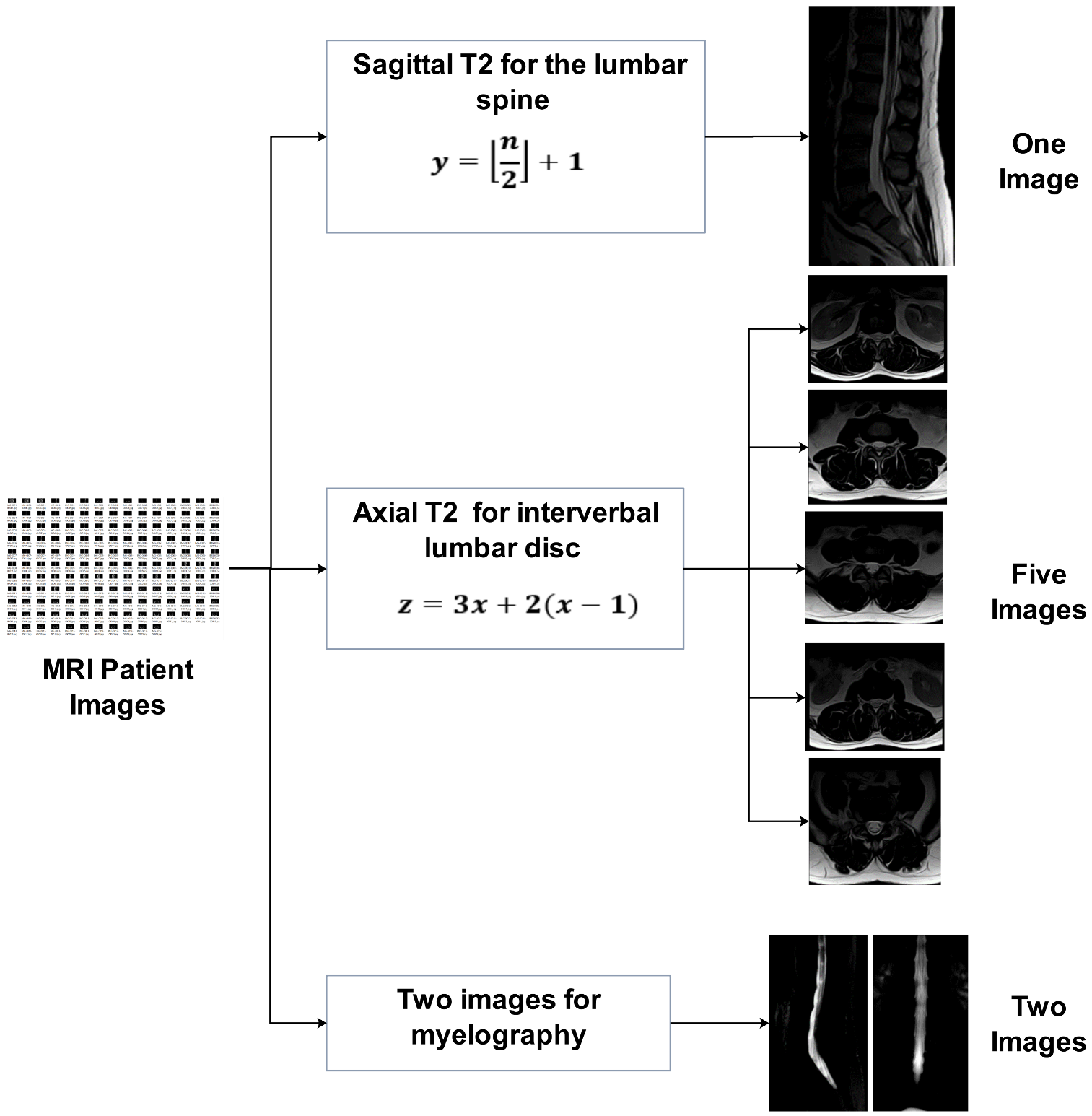
From this group of medical images, we chose 1448 images by applying a novel selection method; with this method, we selected the most essential images (as shown in Figure 1) so that each patient had eight images:

• One image for sagittal view T2 for the lumbar spine.
• Two images for myelography.
• Five images for five intervertebral lumbar disc.

From this massive number of images, the selection process of sagittal view T2 for the lumbar spine was performed according to the following equation:

$$Y=⌊\frac{n}{2}⌋+1$$

(1)

where Y represents the frame number to be selected from the sagittal view T2 (T2-sag) image series and n represents the number of frames in the series. For example, if we have 13 images in T2-sag, we select the seventh image in the sequence.

The selection process for five lumbar spine discs of axial view T2 conducted according to the following equation

$$Z=3x+2(x-1)$$

(2)

where Z represents the frame number to be selected from the lumbar disc axial view T2 image series and x represents the sequence of the intervertebral disc that we want to choose in series, as shown in

Table 1. The selection criteria of the lumbar disc axial view T2 image.

No. (x)	Disc Name	Frame Number to Be Selected
1	L51	$3x+2(x-1)=3\ast 1+2(1-1)=3$
2	L45	$3x+2(x-1)=3\ast 2+2(2-1)=8$
3	L34	$3x+2(x-1)=3\ast 3+2(3-1)=13$
4	L23	$3x+2(x-1)=3\ast 4+2(4-1)=18$
5	L12	$3x+2(x-1)=3\ast 5+2(5-1)=23$

.

This method saves us a lot of time and effort in the process of selecting important images that are used in the classification process, compared with the manual method performed by radiologists, where the images are selected automatically and quickly if this method is applied to the images taken by the magnetic resonance devices to describe the lumbar spine problem.

After we completed the data collection process, we performed the process of naming the data. All data relating to the patient were stored in one folder. We called this folder the name of the identifier taken from the PACS server (IdDevice), as shown in

Table 2. The process of naming data taken from the PACS server.

No.	Images to Be Named	Item’s Name
1	Two images for myelography	IdDevice_1
2		IdDevice_2
3	Sagittial view T2 for Lumbar spine	IdDevice_3
4	Lumbar spine disc L12	IdDevice_12
5	Lumbar spine disc L23	IdDevice_23
6	Lumbar spine disc L34	IdDevice_34
7	Lumbar spine disc L45	IdDevice_45
8	Lumbar spine disc L51	IdDevice_51

. After that, we had 181 folders, in each folder 8 images, and the result was 1448 images.

3.1.3. Labeling the Data with the FaLa Program

The classification system was built for the data to be labeled by the radiologist. Because data without a label is useless, these data were classified by the Department of Radiology at Fallujah Hospital.

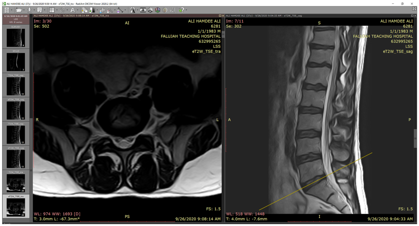
The classification was conducted by using the Fatima Label (FaLa) program. We created the FaLa program to help radiologists perform the labeling process with the help of RadiAnt [40] PACS DICOM viewer. Finally, the patient’s images are displayed on computers (see Figure 2).

As we note in Figure 2, there are several lumbar spine MRI series for each patient, such as survey, Mylo, sagittal T1, sagittal T2, axial T1, axial T2, and so forth. For each series, there are many images, for example, in Axial T2, we have 30 images. So, we are likely to receive 115 DICOMs per patient. In the diagnostic process, radiologists are interested in three series: myelography, axial T2, and sagittal T2.

For each disc level in the lumbar spine, the classification program stores the state of the disc and whether it is herniated or not. In this case, we have four types of the disc: normal, degenerated, bulged, and herniated. In the case that the disc was herniated, there are four types: none, normal, migration, and sequestration. Moreover, the classification program saves the “Spinal Canal Stenosis (SCS), Right Foraminal Stenosis (RFS), and Left Foraminal Stenosis (LFS)” kinds. There are four cases for each stenosis: normal, mild, moderate, and severe.

To store the results of the classification process efficiently, we have graded the data. We have a specific grade for each of the possible states. So, for example, the grade is zero if the lumbar spine disc state is normal, grade one if the lumbar spine disc state is degenerating, grade two if lumbar spine disc state is a bulge, and grade three if lumbar spine disc state is herniated. See

Table 3. The selection criteria of the lumbar disc axial view T2 image.

Grade	Lumbar Spine Disc State	Disc Herniation State	SCS	RFS	LFS
0	Normal	None	Normal	Normal	Normal
1	Degeneration	Normal	Mild	Mild	Mild
2	Bulge	Migration	Moderate	Moderate	Moderate
3	Herniation	Sequestration	Severe	Severe	Severe

to see how we graded the dataset for the lumbar spine MRI.

Table 4. An example of the process of the grading data taken from the PACS server.

Disc Name	Disc State	Type Disc Herniation	SCS	RFS	LFS
L12	0	0	0	0	0
L23	0	0	0	0	0
L34	0	0	0	0	0
L45	2	0	2	0	0
L51	3	2	3	3	3

illustrates the numerical data from classified discs for one patient.

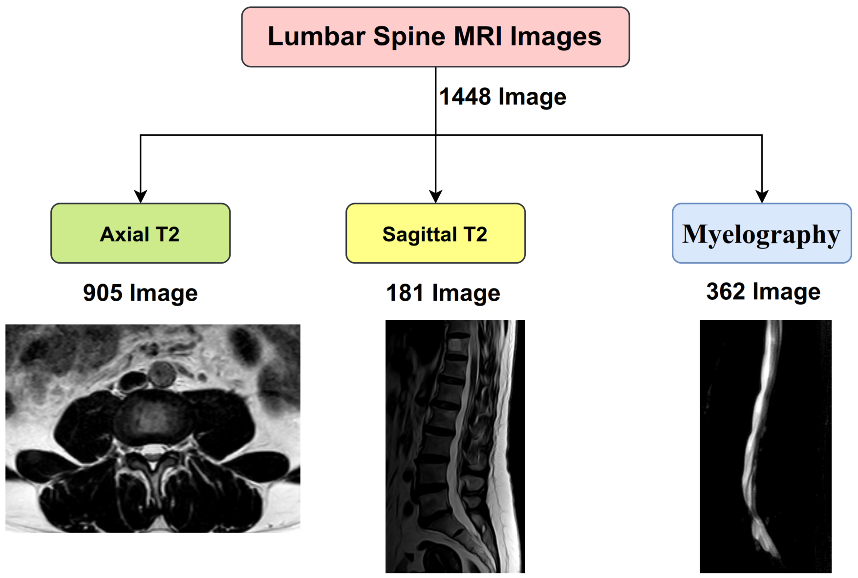
3.2. Analysis of Collected Dataset

After completing the process of collecting and classifying the data, we had 1448 MRI images of the lumbar spine, of which 905 images belonged to the axial T2, 181 belonged to sagittal T2, and 362 belonged to myelography, as shown in Figure 3.

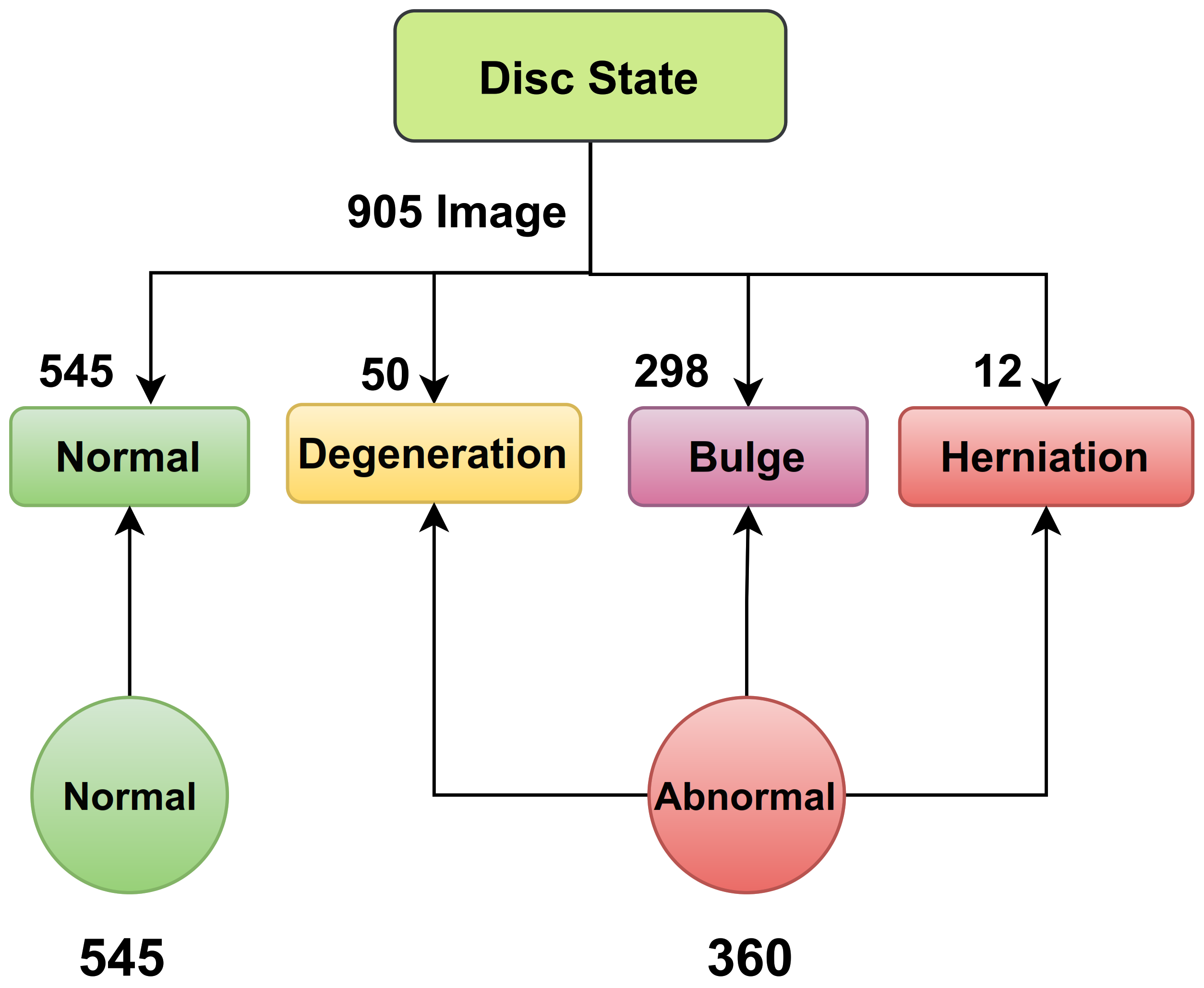
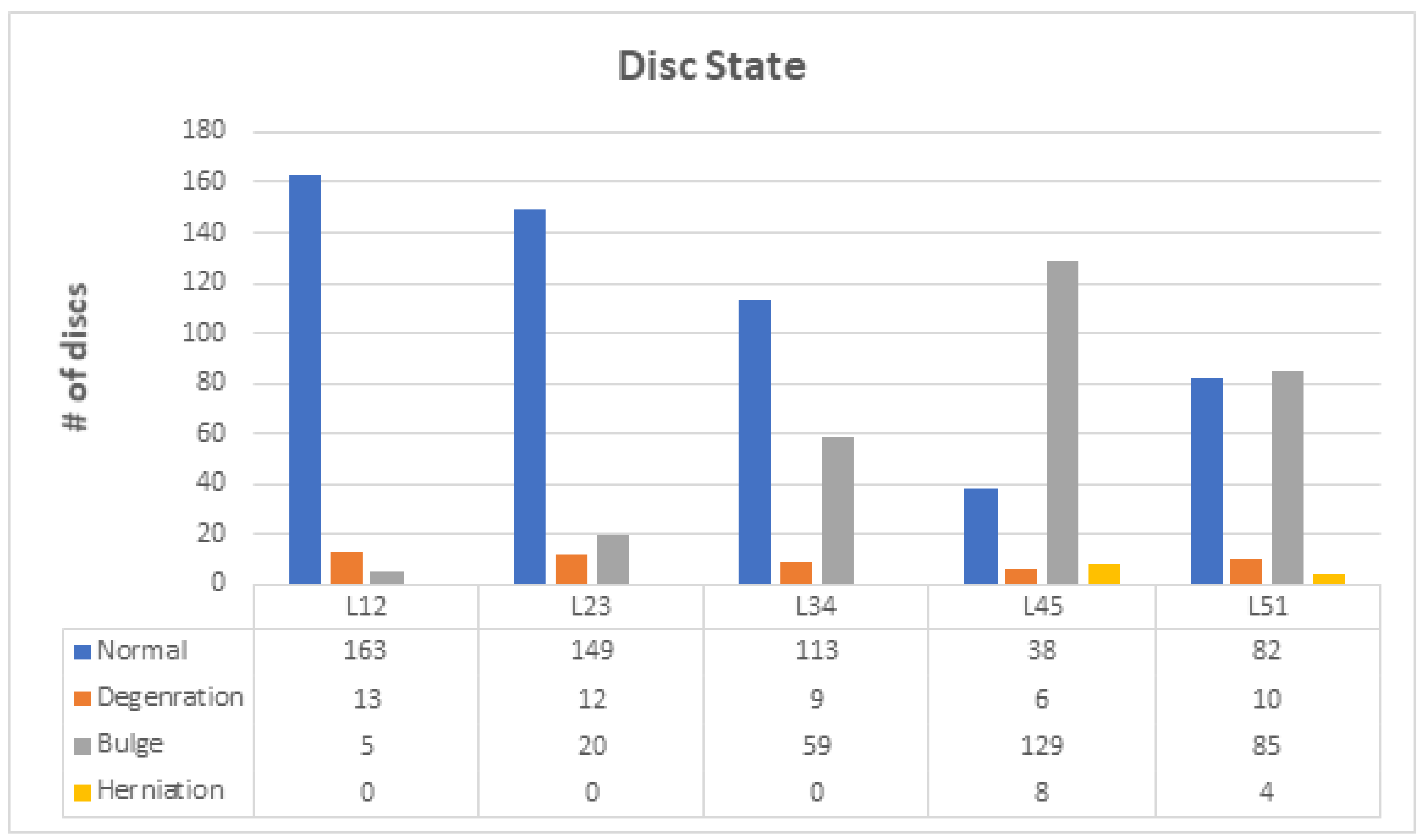
The process of diagnosing lumbar spinal disc state and stenosis depends mainly on axial T2 images. In disc type classification, we had 545 normal, 50 degeneration, 298 bulge, and 12 herniation. These classes can be grouped into two main classes: normal and abnormal. In the normal class we had 545 images, but in the abnormal class (degeneration, bulge, and herniation) we had 360 images, as shown in Figure 4 and Figure 5.

Table 5. Number of disc for each class in disc state.

Disc Name	Normal	Degeneration	Bulge	Herniation
L12	163	13	5	0
L23	149	12	20	0
L34	113	9	59	0
L45	38	6	129	8
L51	82	10	85	4
Total	545	50	298	12

states the number of discs for each class in disc state.

In the case of spinal cord stenosis, we had three classifications: SCS, RFS, and LFS. For SCS, we had 606 normal images, 155 mild images, 85 moderate images, and 59 severe images. For RFS, we had 627 normal images, 140 mild images, 81 moderate images, and 57 severe images. For LFS, we had 628 normal images, 133 mild images, 84 moderate images, and 60 severe images.

3.3. The Proposed ROI

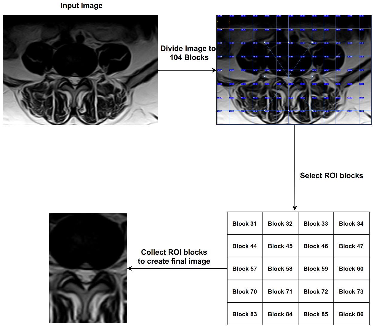
The process of analyzing medical images is very complex and often the parts in the image overlap with the object to be diagnosed. For example, in the process of diagnosing images of lumbar spine discs, there are many shapes in the image such as the image of the intervertebral disc; the same is true in the diagnosis of spinal cord stenosis. Therefore, we proposed the ROI technique, which splits the image into many blocks, and we were able to identify the most important blocks. We divided the image with size (1061 width * 752 height) into 104 blocks and then selected 20 blocks with ROI, each of which has a size (82 * 94). Finally, we chose 20 blocks based on Equation (3).

$$Z=\{30+(13\ast x)+y:x\in \{0,1,2,3,4\},y\in \{1,2,3,4\left\}\right\}$$

(3)

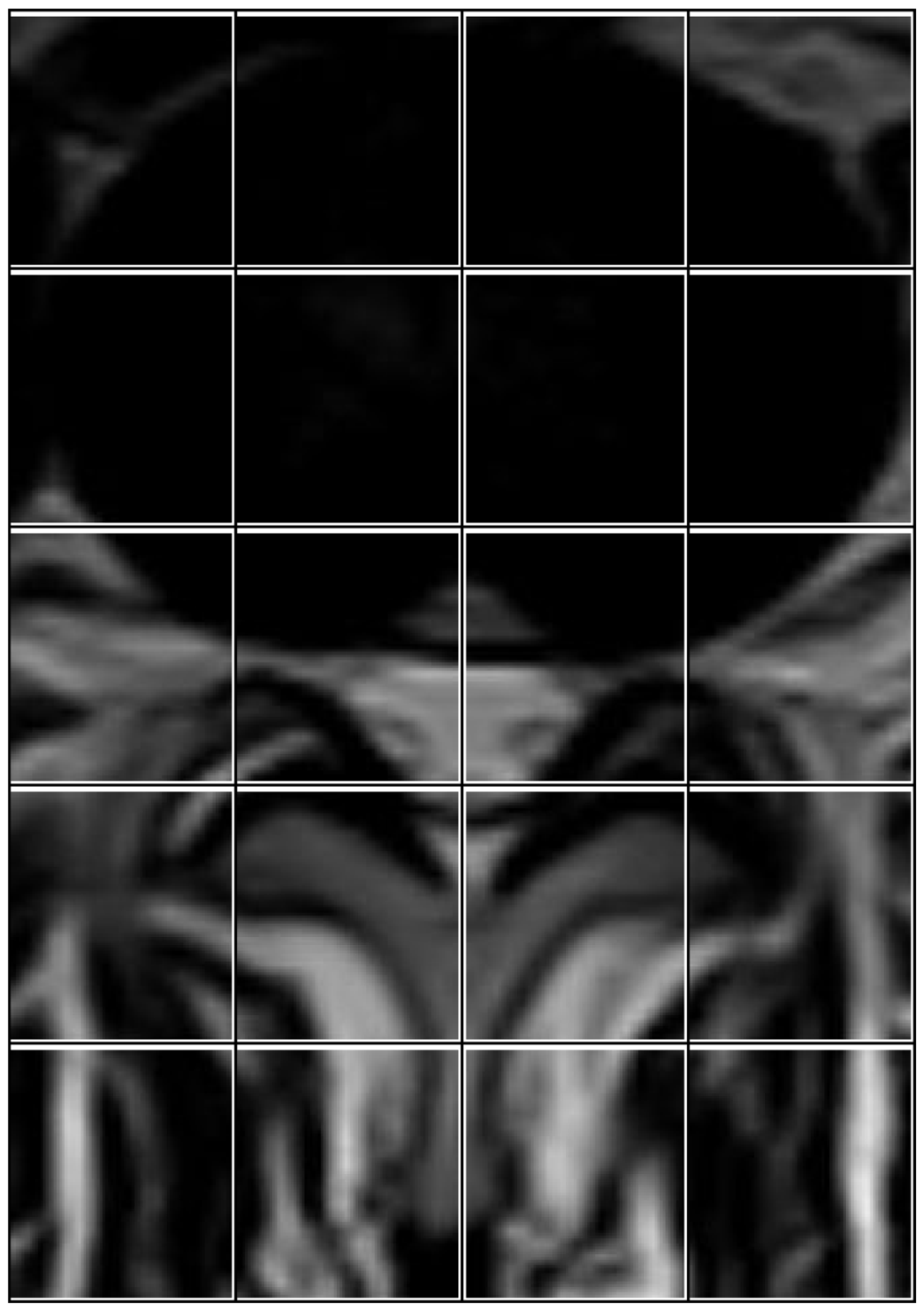
where Z represents the block number to be selected. After completing this process, we obtained images that contain only the area of interest (see Figure 6). In Figure 7, we illustrate the steps to create ROI images.

3.4. Datasets Used in This Work

This section explains the datasets that were used in the proposed model. We used three datasets of MRI medical images. One of them represented the final database, with label data on which the classification process will be carried out. The second described an unlabeled dataset that was used from scratch in the training process. Finally, the third dataset was compiled from several public datasets labeling on brain tumors. Each one is explained below.

• Dataset A: In this dataset, we collected brain tumor MRI images from six public datasets from the Kaggle website, and each database contained a set of labeled images. The first dataset contained 253 MRI images classified into two parts: 98 images without tumors and 155 images with a tumor [41]. The second database included 3264 labeled images divided into four parts. The first part contained 926 images of glioma tumors, the second part contained 937 meningioma tumors, the third part contained 500 images of no tumor, and the last part contained 901 images of pituitary tumors [42]. The third database contained 3060 brain MRI images categorized into three categories: 1500 images containing a tumor, 1500 images without a tumor, and 60 unlabeled images for testing purposes [43]. The fourth database included 7023 labeled images also divided into four categories. The first part contained 1621 images of glioma tumors, the second part contained 1645 meningioma tumors, and the third part contained 2000 images without a tumor, and the last part contained 1757 images of pituitary tumors [44]. The next database included 400 MRI labeled images classified into two categories: 170 normal images (without a tumor) and 230 images with a tumor [45]. The latest database of brain MRI images contained 2501 images classified into two categories: 1551 normal images and 950 images containing stroke [46]. In the end, we grouped these datasets into two classes: normal and abnormal. In the normal class, we had 5819 images, and in the abnormal class, we had 10,622 images. So, in total, we had 16,441 MRI images of brain tumors in this dataset.
• Dataset B: In this dataset, we collected unlabeled MRI images from the PACS server at the Fallujah Teaching Hospital. This dataset had, in total, 209,083 MRI images of the lumbar spine and brain.
• DataSet C: This was our target dataset, built with 181 Lumbar spine patients and containing 1448 images chosen from 21,470 MRI images by applying the novel selection method.

3.5. Hyperparameters

Hyperparameters are essential things that must be determined before starting the training of any model because they control the learning process and are the main pillar on which the model depends. There are some hyperparameter optimization tools, such as Autokeras, that can be used. The following hyperparameters gave us the best results when applied to our dataset.

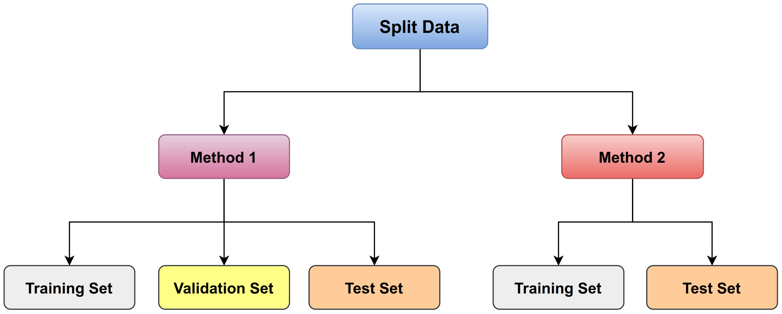
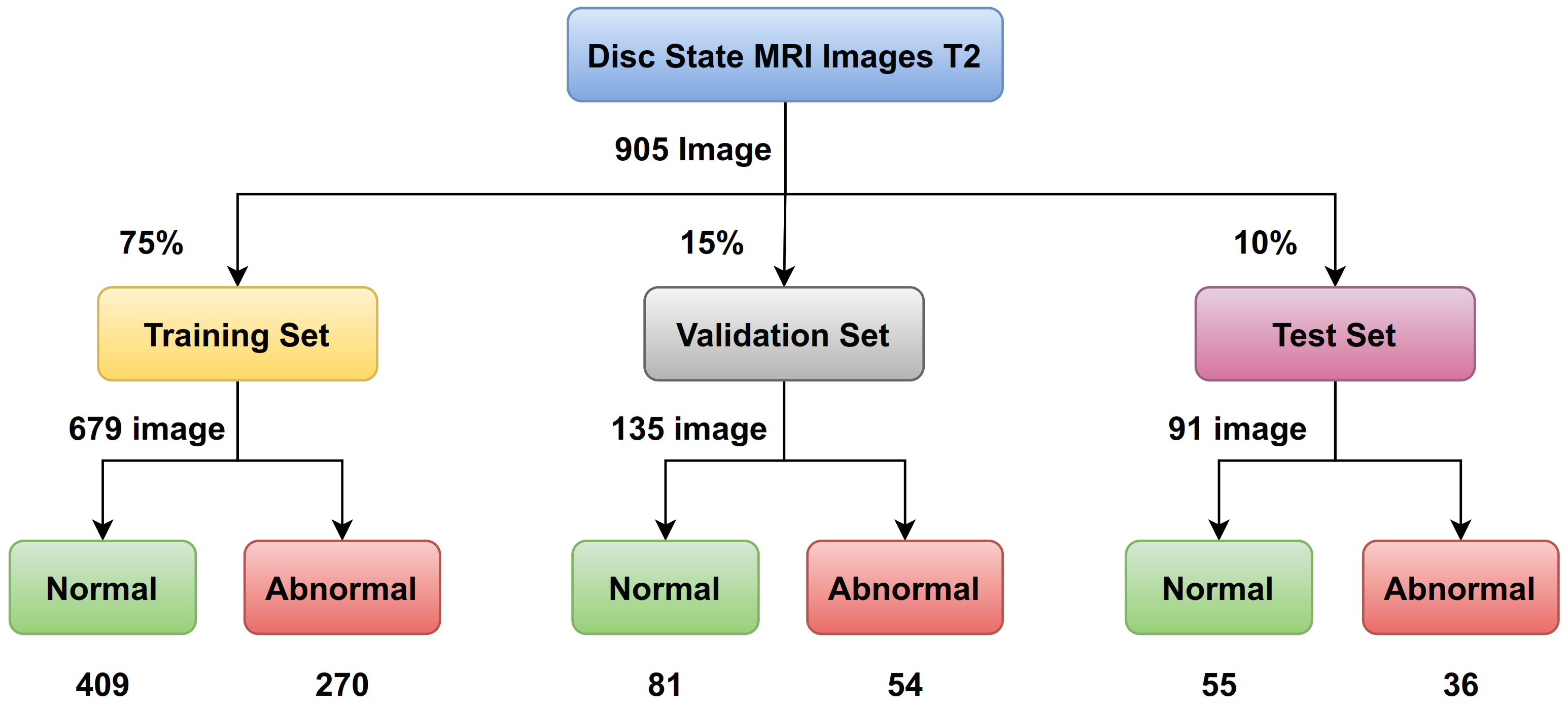
• The train split ratio: There are many methods to determine the criteria. There is a way that MRI images are divided into training and testing only, and another way is that the MRI images are divided into three sets: training, validation, and testing (as shown in Figure 8). In general, we use a ratio of 75% for the training set and 15% for the validation set, and 10% for the testing set for disc state as shown in Figure 9.
• Batch size: In a single forward and backward pass, batch size is the number of training samples counted. The larger the batch size, the more memory space is required. So, the batch size could be 8, 16, 32, 64, 128, and so on. According to our computer hardware memory, we set 64 for batch size.
• Epoch size: One epoch equals one forward and one backward trip through all of the training images. When we apply transfer learning, we set epoch to 50, and when we train from scratch, we set epoch to 100. For instance, if you have 5120 images and a batch size of 64, it will take 80 iterations to finish one epoch.
• Dropout: The essential task of Dropout probability is to prevent overfitting. It enables the model to learn more strong characteristics that can be used with various random subsets of other neurons. We set 0.2 to Dropout.
• The learning rate: The value must be balanced between the very small and the very large value. The small value leads to a slow and incomplete training process. As for the high value, it leads to the instability of the training process. So, when we train any model from scratch, we set $1\mathrm{e}-5$ for learning rate and we set $1\mathrm{e}-3$ for learning rate when we use weights in transfer learning.

3.6. The Proposed Methods

Having enough labeled images to train a deep learning model for medical image classification is a complicated task. Because of the lack of this data and the presence of several complications, some laws in some countries prevent data from being obtained without the person’s consent or allow it to be obtained at a cost.

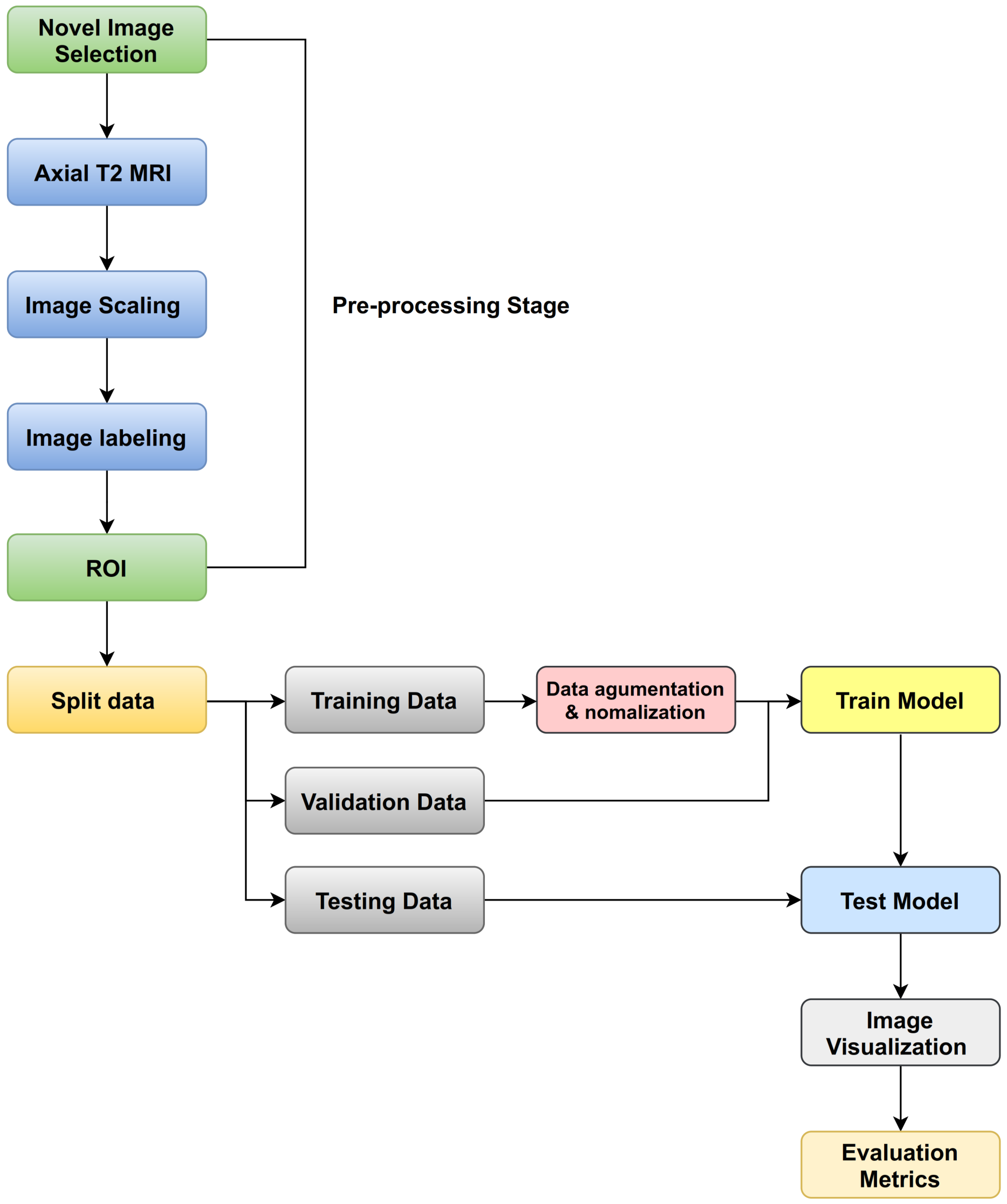
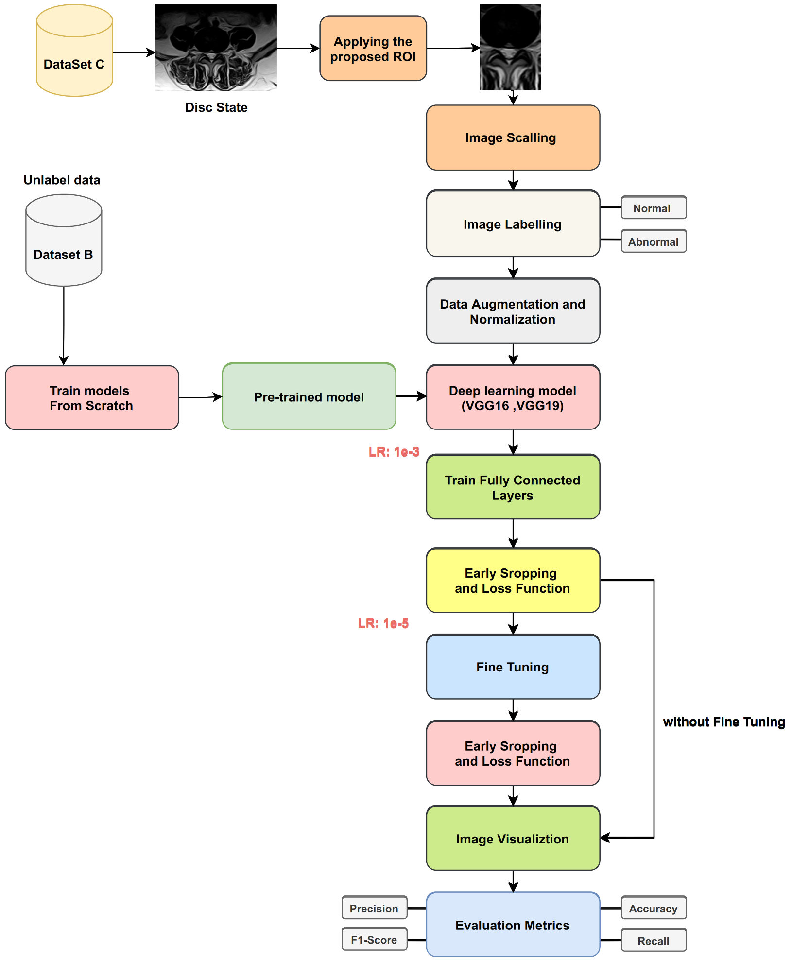
The goals of the following procedures are to solve the problem of lack of training data for lumbar spine classification, to determine the source of the images applied to TL affected in classification task in disc type, and how we can improve the classification task by using proposed techniques, such as ROI. We used four datasets, three as sources applied in TL (ImageNet, Dataset A, and Dataset B) and one as a target (Dataset C). Moreover, we applied various training procedures to the many models (as shown in Figure 10). Our experiments were implemented on Python and the deep learning library Keras using the TensorFlow with PC setup (Intel(R) Core(TM) i9-9900K CPU 3.60 GHz, 32 GB RAM and NVIDIA GeForce RTX 2080 Ti 11GB GPU). Moreover, we proposed three training procedures as follows:

3.6.1. Procedure 1

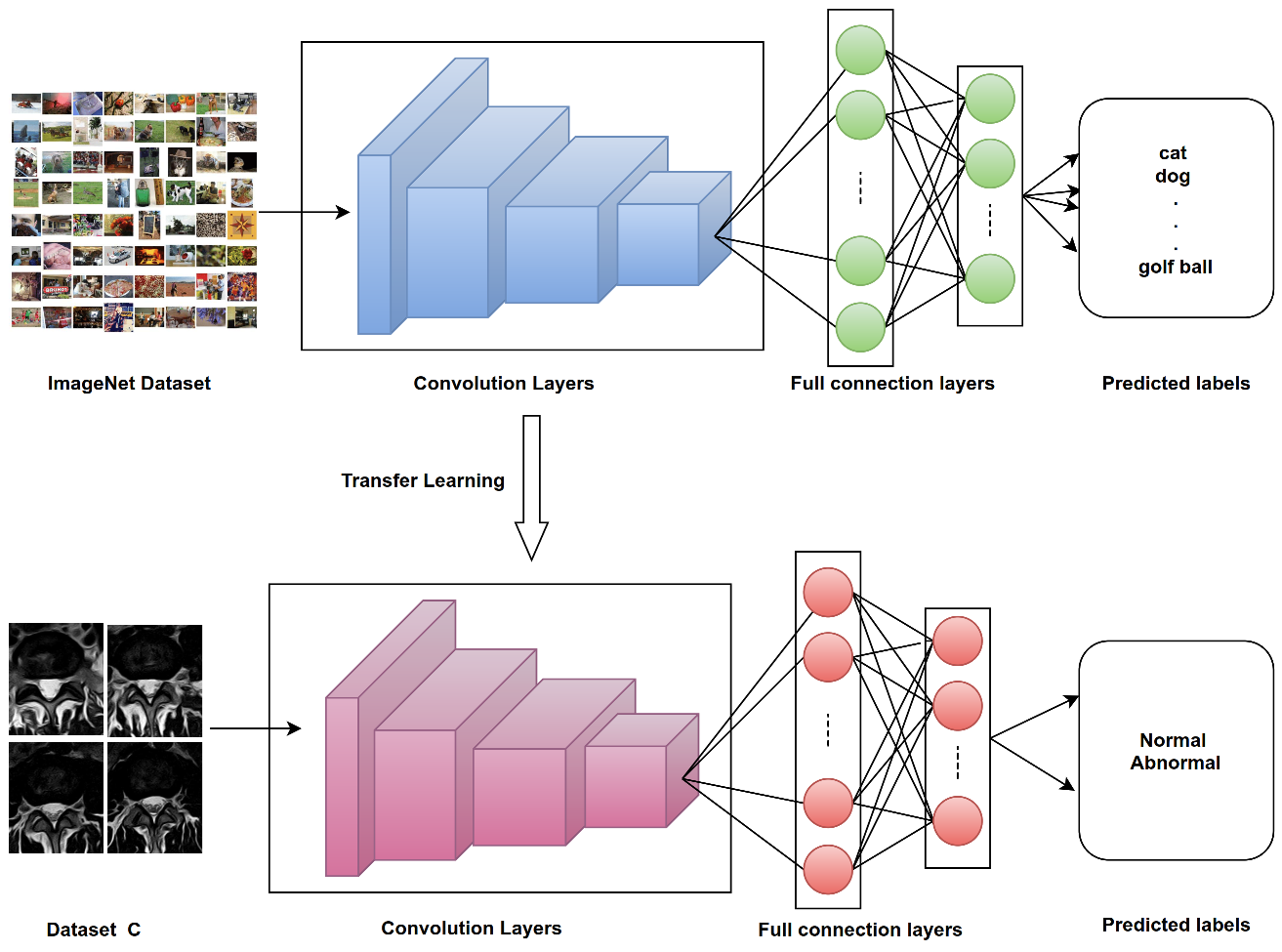
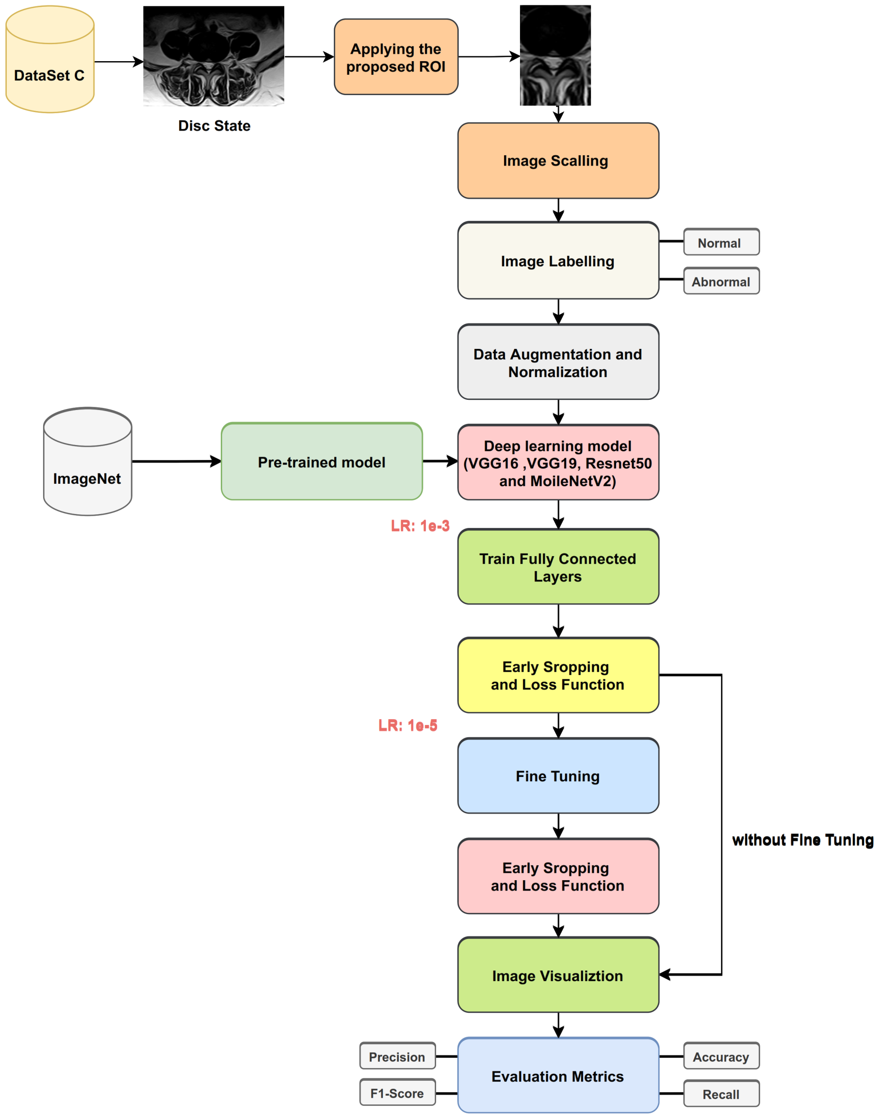
The first procedure applied transfer learning on images from ImageNet (as in Figure 11). We applied four Keras deep learning models (VGG16, VGG19, ResNet50, MobileNet v2) to classify disc state. Finally, we checked the effect of using the proposed ROI on lumbar spine MRI images (as shown in Figure 12).

• Apply transfer learning from ImageNet using four Keras deep learning models without fine-tuning or applying the proposed ROI process.
• Apply transfer learning from ImageNet using four Keras deep learning models with fine-tuning and without applying the proposed ROI process.
• Apply transfer learning from ImageNet using four Keras deep learning models without fine-tuning and with the proposed ROI process.
• Apply transfer learning from ImageNet using four Keras deep learning models with fine-tuning and with the proposed ROI process.

3.6.2. Procedure 2

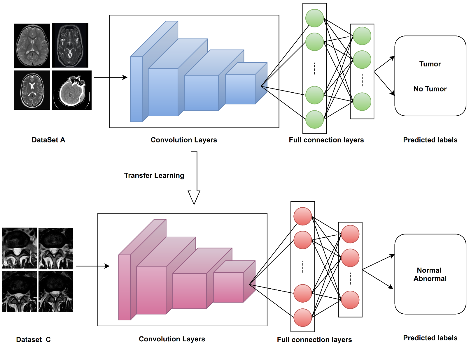
Two Keras deep learning models (VGG16, VGG19) were trained from scratch with Dataset A, and transfer learning was applied to classify disc states in Dataset C with and without fine-tuning (as shown in Figure 13). The key points of the proposed training processes for VGG16 and VGG19 from scratch with Dataset A can be summarized as follows:

• Split Dataset A into two groups ( 85% for training and 15% for validation).
• Choose the hyperparameters’ initial values (eg: learning rate $1\mathrm{e}-5$, batch size = 64, number of epochs = 100).
• To train the model, use the initial values from step 2.
• Use the validation set to evaluate network performance throughout the learning phase.
• For 100 epochs, iterate on steps 3 and 4.
• Choose the model with the lowest error rate on the validation set as the best-trained model.

After training, the VGG16 and VGG19 models from scratch are performed with Dataset A. Then, we transfer learning these weights and use them for training models for disc state classification without fine-tuning. Figure 14 shows transfer learning for disc state classification from label Dataset A. The following steps show the process:

• Split Dataset C into three groups (75% for training, 15% for validation, and 10% for testing).
• Applying the augmentation process (e.g., brightness [0.1, 0.7], horizontal flip, and vertical flip).
• Freeze the pre-trained layers and train only the classifier ( the fully connected layer).
• Choose the hyperparameters’ initial values (e.g., learning rate $1\mathrm{e}-3$, batch size = 64, number of epochs = 50).
• To train the model, use the initial values from step 4.
• Use the validation set to evaluate network performance throughout the learning phase.
• For 50 epochs, iterate on steps 5 and 6.
• Choose the model with the lowest error rate on the validation set as the best-trained model.
• Apply evaluation metrics, such as accuracy, precision, recall, and F1-Score, on the testing set.

With fine-tuning, we performed the same steps above, except in step 3. We did not freeze all pre-trained layers. Instead, we made some layers trainable with two, and we set learning rate $1\mathrm{e}-5$ in step 4.

3.6.3. Procedure 3

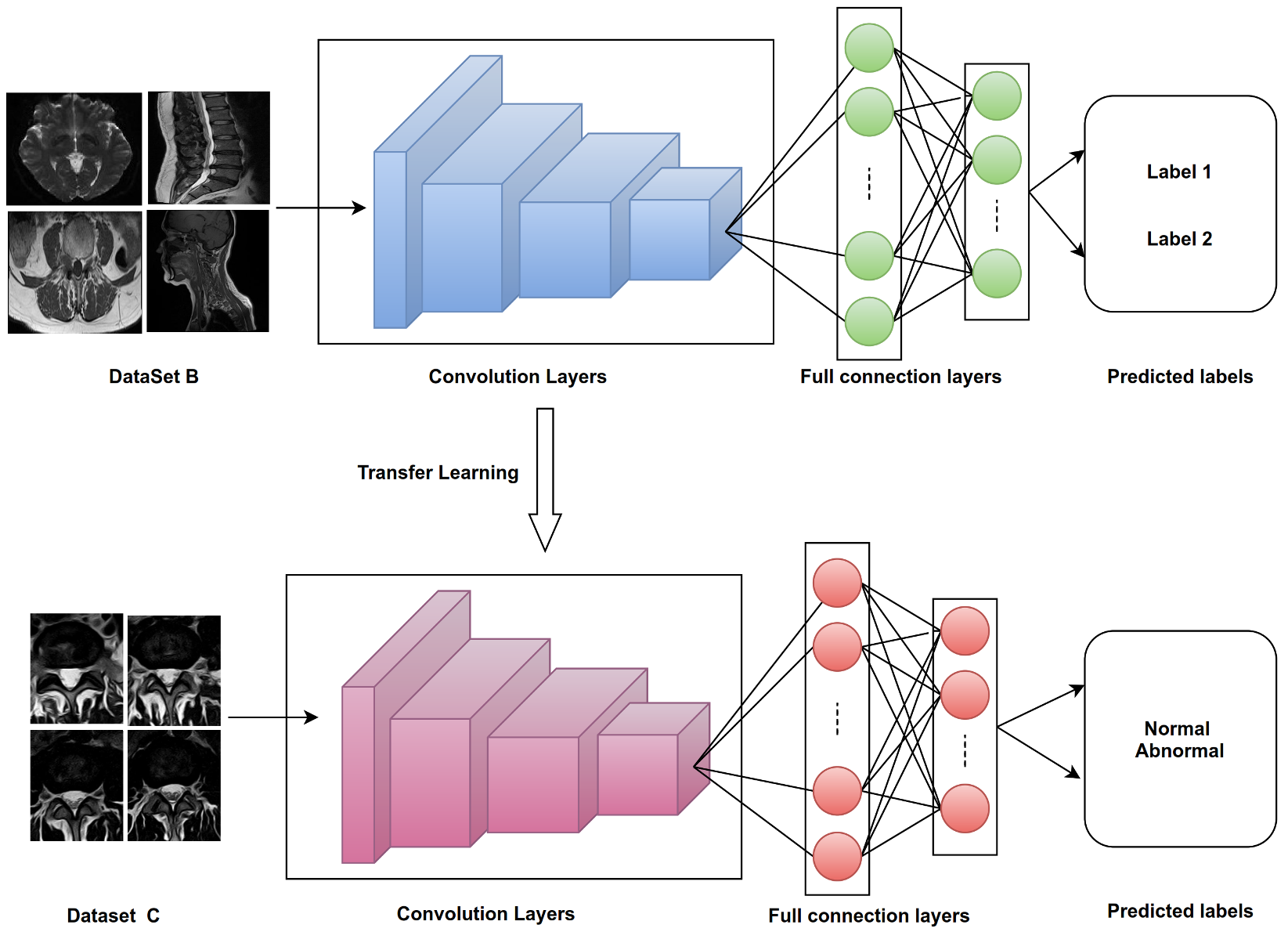
This procedure involved training two deep learning models (VGG16, VGG19) from scratch with Dataset B and applying transfer learning to classify disc states in Dataset C with and without fine-tuning (as Figure 15 indicates). We used the same steps in Procedure 2, expect we used Dataset B for training from scratch. Figure 16 illustrates transfer learning for disc state classification from unlabeled Dataset B.

4. Results

This section will demonstrate the results of applying the three suggested procedures according to the following evaluation metrics.

4.1. Evaluation Metrics

Evaluating the performance or accuracy of any classifier is important as the classifier can perform better against certain metrics; however, it has poor results in others. There are many metrics, and it is important to choose the metrics for the purpose of evaluating the performance of the classifier [47]. Evaluation metrics are mainly used to evaluate the classifier during the training and testing stages. Below are the most popular evaluation metrics. We selected the four types of evaluation metrics that are the most popular, which will be explained below [48].

• Accuracy: The proportion of correct results to the total number of cases tested. It is calculated according to Equation (4):

  $$Accuracy=\frac{(TP+TN)}{(TP+TN+FP+FN)}$$

  (4)
• Recall: Utilized to calculate whether the proportion of actual positives were correctly classified (Equation (5)).

  $$Recall=\frac{TP}{(TP+FN)}$$

  (5)
• Precision: Used to calculate whether the proportion of positives that were correctly predicted is truly positive (Equation (6)).

  $$Precision=\frac{TP}{(TP+FP)}$$

  (6)
• F1-Score: Harmonic mean between recall and precision; the value of the F1-Score is a number between 0 and 1 (Equation (7)).

  $$F1Score=2\ast \frac{(Precision\ast Recall)}{(Precision+Recall)}$$

  (7)

  where, FP = False Positive, TP = True Positive, FN = False Negative, and TN= True Negative. All results in tables are calculated in the percentage units by multiplying each value by 100 to display the results more clearly.

4.2. Results of Procedure 1

In this experiment, we stated the effect of using the proposed ROI on disc state classification. At first, we applied transfer learning from the ImageNet dataset on four deep learning models to classify lumbar spine discs on our data (Dataset C) without applying the proposed method of ROI. When we trained only the fully connected layer without fine-tuning the four models (VGG16, VGG19, ResNet50, and MobileNetV2), we obtained the results in

Table 6. Models with transfer learning from ImageNet for disc state classification without ROI or fine-tuning.

Models	Accuracy (%)	Precision (%)	Recall (%)	F1-Score (%)
VGG19	82.97	80.47	94.50	86.92
ResNet50	77.47	82.69	78.90	80.75
MobileNetV2	79.67	86.73	77.98	82.13
VGG16	78.57	88.89	73.39	80.40

, which prompted us to fine-tune and see how much these results had improved.

After fine-tuning the four models, we noted that the results had not improved significantly as shown in

Table 7. Models with transfer learning from ImageNet for disc state classification without ROI and with fine-tuning.

Models	Accuracy (%)	Precision (%)	Recall (%)	F1-Score (%)
VGG19	84.07	85.09	88.99	87.00
ResNet50	73.63	76.52	80.73	78.57
MobileNetV2	78.57	77.78	89.91	83.40
VGG16	82.42	86.67	83.49	85.05

, and some results have decreased in value as well as in ResNet50. This is due to two reasons. The first is that the models have been trained on data from the ImageNet dataset, and these data are not similar to lumbar spine images. The second reason is that there is a lot of noise in the background, as large parts of the objects in it are similar to the shape of discs.

To improve these results, we applied the proposed ROI method. After its application, we noticed that the results improved significantly. The main objective of this method is to reduce background noise and make the classification process more accurate. The results of this step are shown in

Table 8. Models with transfer learning from ImageNet for disc state classification with ROI and without fine-tuning.

Models	Accuracy (%)	Precision (%)	Recall (%)	F1-Score (%)
VGG19	86.81	92.16	85.45	88.68
ResNet50	83.52	85.71	87.27	86.49
MobileNetV2	81.32	85.19	83.64	84.40
VGG16	84.62	85.96	89.09	87.50

.

After fine-tuning, we obtained the results in

Table 9. Models with transfer learning from ImageNet for disc state classification with ROI and fine-tuning.

Models	Accuracy (%)	Precision (%)	Recall (%)	F1-Score (%)
VGG19	86.81	93.88	83.64	88.46
ResNet50	89.01	89.47	92.73	91.07
MobileNetV2	84.62	83.61	92.73	87.93
VGG16	84.62	88.68	85.45	87.04

, which show the importance of applying this method and how it improved results. The application of this method improved the disc state classification results in VGG19 2%, ResNet50 16%, MobileNetV2 5%, and VGG16 2%, as shown in

Table 10. Improvement rate after applying the proposed ROI to disc state.

Models	F1-Score before ROI (%)	F1-Score after ROI (%)	Improvement Rate (%)
VGG19	87.46	88.46	2
ResNet50	78.57	91.07	16
MobileNetV2	83.4	87.93	5
VGG16	85.05	87.04	2

. This rate was measured by the following equation:

$$Y=\frac{x_2-x_1}{\left|x_1\right|}\times 100\%$$

(8)

where $x_1$ is old value and $x_2$ is new value.

4.3. Results of Procedure 2

To improve classification results and solve the problem of no significant correlation between images in ImageNet with images of the lumbar spine, we trained two deep learning models (VGG16 and VGG19) from scratch using medical images classified in (Dataset A) that are similar to the images of the lumbar spine. Then, we used transfer learning from (Dataset A) to classify disc state. When training only fully connected layers, we obtained the following results: accuracy 78.02%, 73.97% precision, 98.18% recall, and an F1-Score of 84.38% in the VGG16 model; 80.42% accuracy, 84.21% precision, 87.27% recall, and an F1-Score of 85.71% in the VGG19 model. After fine-tuning, we obtained 87.91% accuracy, 89.29% precision, 90.91% recall, and an F1-Score of 90.09% in the VGG16 model; 87.91% accuracy, 87.93% precision, 92.73% recall, and an F1-Score of 90.27% in the VGG19 model, as shown in

Table 11. Models with transfer learning from Dataset A (labeled brain tumors) for disc state classification.

Models	Accuracy (%)	Precision (%)	Recall (%)	F1-Score (%)
VGG16
Without Fine-Tuning	78.02	73.97	98.18	84.38
With Fine-Tuning	87.91	89.29	90.91	90.09
VGG19
Without Fine-Tuning	80.42	84.21	87.27	85.71
With Fine-Tuning	87.91	87.93	92.73	90.27

.

As we note in

Table 12. Improvement rate after transfer learning from labeled data (Dataset A).

Models	F1-Score for TL from ImageNet (%)	F1-Score for TL from Dataset A (%)	Improvement Rate (%)
VGG16	87.00	90.09	4
VGG19	85.05	90.27	6

, the results improved in VGG16 4% and in VGG19 6%, compared with transfers from ImageNet. This is because the images in Dataset A are closer to lumbar spine MRI than the images from ImageNet.

4.4. Results of Procedure 3

The hardest part of building a deep learning model for medical image classification is having enough labeled images to train the model. However, in most cases, these data are not available. Therefore, through this hypothesis, we show the usefulness of training deep learning models on unlabeled data. The goal of this procedure was to train the existing filters in the convolution layers that are responsible for extracting features from images. We trained two deep learning models (VGG16 and VGG19) from scratch using unlabeled medical images in Dataset B, which were similar to the images of the lumbar spine. Then, we used transfer learning from Dataset B to classify disc state in Dataset C. When training only fully connected layers, we obtained the following results: 80.22% accuracy, 77.61% precision, 97.55% recall, and an F1-Score of 85.25% in the VGG16 model; 85.71% accuracy, 85.00% precision, 92.73% recall, and an F1-Score of 88.70% in the VGG19 model. After we used fine-tuning, we obtained 89.01% accuracy, 90.91% precision, 90.91% recall, and an F1-Score of 90.91% in the VGG16 model; 87.91% accuracy, 90.74% precision, 89.09% recall, and an F1-Score of 89.91% in the VGG19 model, as shown in

Table 13. Models with transfer learning from Dataset B (unlabeled data) for disc state classification.

Models	Accuracy (%)	Precision (%)	Recall (%)	F1-Score (%)
VGG16
Without Fine-Tuning	80.22	77.61	97.55	85.25
With Fine-Tuning	89.01	90.91	90.91	90.91
VGG19
Without Fine-Tuning	85.71	85.00	92.73	88.70
With Fine-Tuning	87.91	90.74	89.09	89.91

.

As we noticed in

Table 14. Improvement rate after transfer learning from unlabeled data (Dataset B).

Models	F1-Score for TL from ImageNet (%)	F1-Score for TL from Dataset B (%)	Improvement Rate (%)
VGG16	87.00	90.91	4
VGG19	85.05	89.91	6

, the results improved in VGG16 4% and in VGG19 6%, compared with TL from ImageNet. This is because the images in Dataset B are closer to lumbar spine MRI than the images from ImageNet.

In some cases, the performance and F1-Score degraded, such as ResNet50 (in Table 6 and Table 7) and VGG19 (in Table 8 and Table 9), because the target dataset (dataset C) is dissimilar to the ImageNet dataset.

In Table 11 and Table 12, VGG16 improved, but VGG19 improved little because VGG19 has more parameters than VGG16. So, it required more data than VGG16 to train these large parameters.

In all tables, we depend on the F1-Score rather than accuracy as in Table 13; the accuracy of VGG19 is quite higher than that of VGG16 without pretraining (80.22 and 85.71). However, the accuracy of VGG19 is even lower than that of VGG16 (89.01 and 87.91), but we depend on F1-Score improvement because we have unbalanced classes.

5. Discussion

Deep learning algorithms have become one of the most popular methods and forms of algorithms used to diagnose the LPB in the lumbar spine.

Our approach applies various training procedures to the many models (VGG16 and VGG19) to classify the disc state. Most of the research for disc state classification used CNN models. It is known that CNN models require large amounts of data for training. The most critical challenge facing these models is the lack of data to train them. Collecting a large amount of labeled data is very difficult, especially medical data. TL on many datasets used to solve the lack of training data for lumbar spine classification.

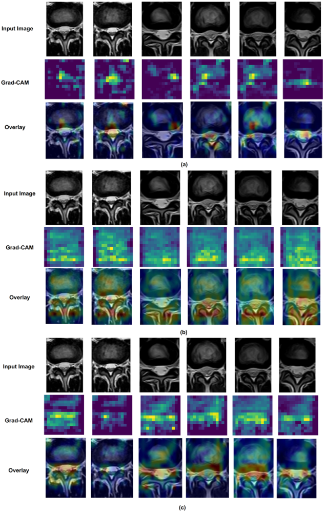
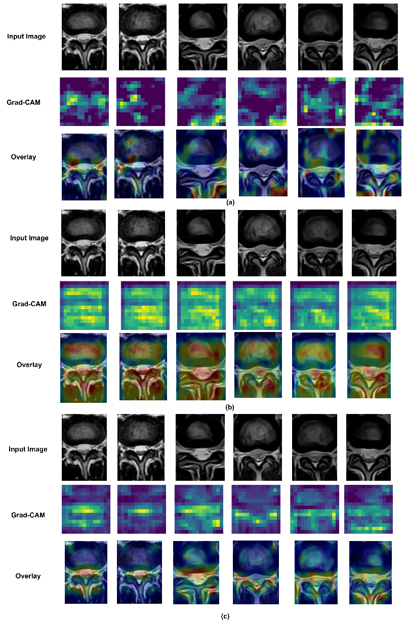
We also used the Grad-CAM [49] visualization technique on deep learning models (VGG16 and VGG19) for disc state classification to make these models more explainable. In Grad-CAM, the last convolutional layer in the model is used to create heat maps. The heat map for the last convolutional layer should show the model’s best accurate visual description of the object. Figure 17 shows Grad-CAM using VGG16 for disc state classification TL from ImageNet, Dataset A (labeled data), and Dataset B (unlabeled data). As we note, there were some important differences when VGG16 TL is applied from each dataset; the most significant regions in the image predicted better VGG16 TL from unlabeled data than ImageNet. Moreover, in Figure 18, the most important regions in the image predicted better VGG19 TL from unlabeled data than ImageNet.

6. Conclusions

This paper proposed a lumber spine disc classification approach using transfer learning. This approach can be highlighted into the following stages: (i) The application of the novel selection method saved us a lot of time, as the selection process was performed manually in the past. Now, this process is performed automatically, which accelerates the process of building the dataset on the subject of the lumbar spine. (ii) The selected images will be used in the classification process using the constructed FaLa. The expert used the FaLa to classify the disc state. The FaLa made the classification process easier for experts. Furthermore, FaLa enabled us to efficiently obtain the data in a digital form to complete the classification process. (iii) Regarding the pre-processing stage, the proposed ROI applied on images achieved better results when we applied it in disc state classification. In the process of diagnosing images of lumbar spine discs, there were many shapes in the image overlapping with the thing to be analyzed, such as the image of the intervertebral disc in the case spinal cord stenosis diagnosis. (iv) Applying the proposed ROI method improved the disc state classification results in VGG19 2%, ResNet50 16%, MobileNetV2 5%, and VGG16 2%. (v) Three procedures and from-scratch training models were applied using two datasets: Dataset A (16,441 labeled MRI images of brain tumors) and Dataset B (209,083 unlabeled MRI images of the lumbar spine and brain), and applied transfer learning from ImageNet, Dataset A, and Dataset B increased the efficiency of the classification process in Dataset C. (vi) The closer the data to be classified to the data that the system is trained on, the better the results. (vii) If classified data are available in large numbers, it is better than unclassified data. However, this is difficult to obtain, especially for medical images. (viii) The results improved in VGG16 4% and in VGG19 6%, compared with transfers from ImageNet. This is because the images in Datasets A and B were more similar to lumbar spine MRI than the images from ImageNet.