Optimized Operation of Integrated Energy Microgrid with Energy Storage Based on Short-Term Load Forecasting

Abstract

This research proposes an optimization technique for an integrated energy system that includes an accurate prediction model and various energy storage forms to increase load forecast accuracy and coordinated control of various energies in the current integrated energy system. An artificial neural network is utilized to create an accurate short-term load forecasting model to effectively predict user demand. The 0–1 mixed integer linear programming approach is used to analyze the optimal control strategy for multiple energy systems with storage, cold energy, heat energy, and electricity to solve the problem of optimal coordination. Simultaneously, a precise load forecasting method and an optimal scheduling strategy for multienergy systems are proposed. The equipment scheduling plan of the integrated energy system of gas, heat, cold, and electricity is proposed after researching the operation characteristics and energy use process of the equipment in the combined power supply system. A system economic operation model is created with profit maximization in mind, while also taking into account energy coordination between energy and the power grid. The rationality of the algorithm and model is verified by analyzing the real data of a distributed energy station in Wuhan for two years.

1. Introduction

Energy scarcity is a major concern for the world today. The increasing use of fossil energy contributes to a number of environmental issues, including global warming and environmental devastation [1,2]. On the one hand, governments around the world are actively researching new energy sources to replace fossil fuels [3]. On the other hand, as science and technology advance, the number of different types of power facilities and the share of renewable energy in the energy supply grows by the day, and the types of energy supply in the power system diversify [4]. Due to the uncertainty of various forms of user loads, the system must be adjusted, and energy generation and storage must be altered in accordance with user needs. Multienergy complementarity can enable peak and valley filling of energy supply while also providing the most economic gain. As a result, it is critical to develop a integrated energy system. The randomness of the energy supply side is increased and controllability is reduced as a result of the construction of a large number of integrated energy systems [5]. As a result, it is vital to expand the demand analysis of various energy sources and the schedule analysis of each piece of equipment, with the creation of a regional integrated energy system being particularly important [6,7].

At the moment, integrated energy system research is mostly focused on system analytic modeling and optimal scheduling. Many academics conducted extensive research on integrated energy systems. In terms of the structure of an integrated energy system, literature [8] presents a system model that takes into account electrical and thermal load and establishes a multiobjective operation optimization method with economic gain and comprehensive energy efficiency as the goal function. The literature [9] established a planning model for an electric-hydrogen integrated energy system (EH-IES) and investigated the system’s optimal scheduling. Literature [10,11] provides a multienergy complementarity-based complete demand response strategy, although it is confined to combined thermoelectric dispatching. Literature [12] investigates the grid-connected structural strategy of a distributed photovoltaic energy storage system. In terms of optimal scheduling, the literature [13] offered a two-stage optimal operating technique for the integrated energy system, which includes cold, heat, and electricity. The literature [14] proposes a two-layer optimal scheduling technique for community integrated energy systems (CIES) and electric vehicle charging stations (EVCS). The MILP algorithm is used in the literature [15] to investigate the optimal scheduling strategy of an integrated energy system with CCHP and wind power generation. The literature [16] proposed an optimization approach for an integrated energy system that takes into account demand responsiveness and thermal comfort, and it used the NSGA-II algorithm for this system’s optimization study.

Constructing an accurate prediction model is a critical component of developing an integrated energy system. Peak load reducing and valley filling can be accomplished by developing a accurate load prediction model [17]. It can not only fulfill peak energy demand while lowering production costs, but it can also decrease system capacity [18]. Literature [19,20,21] investigates the optimization of a distributed integrated energy system and chooses a typical day in different seasons to maximize the system results. The literature [20] has explored the impact of energy storage on the operation of an integrated energy system in various grid-connected modes, but only typical day load is addressed, making usage in the actual system impractical. The author identified a typical summer day as an appropriate regional scheduling scheme for optimal scheduling of multienergy systems in reference [22]. The literature [23] outlines modern energy system modeling, and current user-side prediction modeling mostly focuses on power prediction. Wind power generation and solar power generation are forecasted in the literature [24,25,26] by developing an accurate power prediction model.

The majority of the previous research focused on the optimal scheduling of integrated energy systems. Typical daily data are utilized to anticipate loads for optimization, or real-world data are used directly for analysis without an exact load prediction. At the moment, the integrated energy system prediction research focus is on the power forecast of new energy generation equipment and the power system user load prediction. Other types of energy load prediction research are currently in short supply. At the same time, the current integrated energy system makes use of a limited number of energy types and energy storage forms [27].

Based on this, this work addresses both optimization scheduling and load prediction in the integrated energy system, and incorporates various types of energy storage to increase the economic optimization scheduling interval and provide more operation scenarios. Based on short-term load forecasting, a day-to-day optimal scheduling method for a multienergy microgrid with energy storage is proposed. The user load of diverse energy types can be properly predicted by developing an accurate load prediction model. The MILP model of the integrated energy system was built with the optimization of comprehensive income as the goal function, taking into account the interaction between diverse energy sources and the power grid, multienergy coordination, and dynamic balance. Finally, using a specific example, this research analyzes the actual situation and data of a park in Wuhan, and confirms the feasibility and economy of the proposed model and optimization technique. Unlike traditional research, the algorithm model developed has practical application value and can be immediately applied to the prediction and optimization of actual energy stations [28].

The contributions of this paper are summarized as follows:

(1) An accurate model of the user’s cooling, heating, and electrical load is established, laying the groundwork for system optimization to follow.

(2) In the integrated energy system, consider additional types of energy, solve the coupling problem of different types of energy, add more types of energy storage, and broaden the optimization range.

(3) A comprehensive energy system optimization strategy based on precise load prediction is proposed by merging prediction and control. This strategy improves the feasibility of optimal scheduling results and can be used to practical projects when compared to traditional typical daily optimization.

2. System Description

Figure 1 depicts a typical multienergy system, which includes both production equipment and energy storage equipment. The main chemical energy into electricity and gas energy input, energy conversion process equipment used primarily for two miniature gas internal combustion engines, two flue gas type lithium bromide units, three sets of centrifugal water chilling unit, lithium bromide unit including waste heat recovery equipment. Because of the substantial difference in cooling and heating, the two modules are modeled separately in the future modeling of the lithium bromide unit Figure 1.

The scheduling techniques of determining electricity by heat and determining heat by electricity, as well as the scheduling method of adding cold and heat storage, are all considered in this study. Because of the addition of a cold and thermal energy storage tank, storage can be done ahead of time in the scheduling process based on the user’s cold and heat demand, reducing the start and stop or dispatching times of the internal combustion engine and lithium bromide unit. Adding several energy storage devices can expand the integrated energy system’s scheduling scope, changing the current situation where the system can only be optimized by changing the production equipment’s output. This update expands the scheduling options for the integrated energy system Figure 2.

3. Methodology

3.1. Equipment Modeling Analysis

To tackle the integrated energy system optimization problem, it is important to model the energy system’s production and storage equipment. The system scheduling is optimized using the mathematical model. This study establishes the mathematical model of the equipment and the revenue model of some equipment based on the equipment presented in the previous section.

(1) Gas Internal Combustion Generator

The waste heat from an internal combustion engine is made up of three basic components. The first component is cooling water for the cylinder liner, the second half is cooling water for the lubricating oil, and the third part is smoke exhaust heat. The three parts of energy that can be recovered by the recovery equipment are united to simplify the model. As a result, a mathematical model of gas internal combustion engine energy conversion can be created. The following is the model of a gas internal combustion generator:

$$E_{GE}={\eta }_{GE}{G}_{GE}{\delta }_{GE}$$

(1)

$$Q_{exh}={\eta }_{RE}{G}_{GE}{\delta }_{GE}$$

(2)

In Formula (1), $E_{GE}$ denotes the electric energy created by the gas internal combustion engine in kWh, and $G_{GE}$ denotes the natural gas heat flow rate in m³/h. ${\eta }_{GE}$ denotes the gas internal combustion generator’s electric energy conversion efficiency. The waste heat recovery efficiency of an internal combustion generator is ${\eta }_{RE}$ in Formula (2). The available heat energy provided by a gas internal combustion generator, kJ, is represented by $Q_{exh}$. $Q_{exh}$ is divided into three parts. Waste heat recovery unit absorption portion, absorption chiller absorption part, and unused escape component. This is where the $\delta$ notion is presented. The logical variable $\delta$ denotes the equipment’s start and stop, while ${\delta }_{GE}$ represents the gas internal combustion generator’s start and stop.

The economic model of internal combustion engine is established according to its working conditions:

$$C_{GE}=p_{repair}{E}_{GE}+p_f\left(t\right)G_{GE}$$

(3)

where $p_f\left(t\right)$ represents the natural gas price at time t. $p_{repair}$ represents the unit maintenance cost. $C_{GE}$ represents the operating cost of the internal combustion engine.

(2) Lithium Bromide Absorption Refrigeration Unit

In a combined power supply system, a waste heat absorption chiller is essential. It is a critical piece of equipment for increasing the overall efficiency of energy use and the system’s overall performance. To carry out refrigeration, a lithium bromide refrigerator collects high temperature exhaust from power producing equipment, but it must also consume a certain quantity of electricity.

The following is the model of a lithium bromide absorption refrigerator:

$$Q_{LB\_C}={\eta }_{LB\_C}{Q}_{exh,1}{\delta }_{LB\_C}$$

(4)

$$C_{LB\_C}=p_{buyE}\left(t\right)E_{LB\_C}$$

(5)

The refrigerating capacity of a lithium bromide absorption refrigerator is $Q_{LB\_C}$, in kJ. The part of the available heat energy provided by the gas internal combustion generator that is absorbed by the lithium bromide absorption chiller, kJ, is represented by $Q_{exh,1}$. The conversion efficiency of the lithium bromide absorption chiller is represented by ${\eta }_{LB\_C}$, and the start and stop of the lithium bromide absorption refrigerator is indicated by ${\delta }_{LB\_C}$. The purchase price of power at time t is represented by $p_{buyE}\left(t\right)$. The cold operation cost of the bromine mechanism is represented by $C_{LB\_C}$. The power consumption of a lithium bromide absorption chiller is represented by $E_{LB\_C}$.

(3) Centrifugal Water-Cooling Unit

Large refrigerating capacity, small volume, small mass, steady operation, and no oil compression are all properties of centrifugal refrigeration compressors, which are commonly employed in large refrigeration air conditioning and heat pump systems. Refrigeration is achieved by centrifugal refrigerators using electric energy, and its mathematical model is as follows:

$$Q_{EC}={\eta }_{EC}{E}_{EC}{\delta }_{EC}$$

(6)

$$C_{EC}=p_{buyE}\left(t\right)E_{EC}$$

(7)

where $Q_{EC}$ represents the centrifugal refrigerator’s refrigerating capacity in kJ, $E_{EC}$ represents the electrical energy consumed by the centrifugal refrigerator in kWh, and ${\eta }_{EC}$ represents the centrifugal refrigerator’s conversion efficiency in percent. The start and stop times of the centrifuge are indicated by ${\delta }_{EC}$. The cost of the centrifugal water-cooling unit is represented by $C_{LB\_C}$.

(4) Waste Heat Recovery Device

Heat recovery by residual heat recovery of lithium bromide unit is primarily accomplished in this issue by absorption of heat emitted from the gas internal combustion generator by the lithium bromide unit’s residual heat recovery unit. Because of the varied refrigeration and heating models, the refrigeration and heating are modeled independently, and the model of the residual heat recovery unit is as follows:

$$Q_{LB\_H}={\eta }_{LB\_H}{Q}_{exh,2}{\delta }_{LB\_H}$$

(8)

$$C_{LB\_H}=p_{buyE}\left(t\right)E_{LB\_H}$$

(9)

The heat generated by the waste heat recovery device is represented by $Q_{LB\_H}$. $Q_{exh,2}$ denotes the amount of useful heat energy absorbed by the waste heat recovery mechanism from the gas internal combustion generator. The energy recovery efficiency of the waste heat recovery device is represented by ${\eta }_{LB\_H}$. The start or stop of the waste heat recovery equipment is indicated by ${\delta }_{LB\_H}$. The running cost of the waste heat recovery unit is represented by $C_{LB\_H}$. The power consumption of the waste heat recovery device is represented by $E_{LB\_H}$.

(5) Energy Storage Device

It is difficult to model energy storage technology. This study analyzes energy storage equipment as an electrical/thermal/cooling load when linked to the comprehensive energy system for charging to simplify the model and make it easier to understand. It can be thought of as a distributed electricity/heat/cold source when releasing energy. The generic energy model for charging and discharging energy storage equipment was established. The mathematical model of heat and cold storage equipment is described in the following formula.

$$Q_C=Q_{sC}\left(0\right)+\sum _{t\in {\Phi }_{in}}{Q}_{sC}\left(t\right){\eta }_{C,in}\Delta t-\sum _{t\in {\Phi }_{out}}{Q}_{uC}\left(t\right){\eta }_{C,out}\Delta t-Q_1\Delta t$$

(10)

$$Q_H=Q_{sH}\left(0\right)+\sum _{t\in {\Phi }_{in}}{Q}_{sH}\left(t\right){\eta }_{H,in}\Delta t-\sum _{t\in {\Phi }_{out}}{Q}_{uH}\left(t\right){\eta }_{H,out}\Delta t-Q_2\Delta t$$

(11)

In Formula (10), $Q_C$ denotes the energy stored by the current water tank’s cold energy storage, kJ. $Q_{sC}\left(t\right)$ and $Q_{uC}\left(t\right)$ denote the energy stored and released by the energy storage tank at time t, and kJ. ${\eta }_{C,in}$ and ${\eta }_{C,out}$ denote the efficiency of energy storage and energy storage release, respectively. The time it takes to carry out or release the energy storage is represented by $\Delta t$. The energy dissipation rate of the storage tank, kJ, is represented by $Q_1$.

The energy held by the current water tank’s cold energy storage is represented by $Q_H$ in Formula (11). The energy stored and released by the energy storage tank at time t are represented by $Q_{sH}\left(t\right)$ and $Q_{uH}\left(t\right)$, respectively. The efficiency of energy storage and the efficiency of energy storage release are represented by ${\eta }_{H,in}$ and ${\eta }_{H,out}$, respectively. The time it takes to carry out or release the energy storage is represented by $\Delta t$. The energy dissipation rate of the storage tank is represented by $Q_2$.

3.2. System Optimization Analysis

3.2.1. The Objective Function

The maximum daily revenue is considered as the objective function of the integrated energy system’s optimal operation under the assumption of contemplating the maximum economic advantage. The daily cost is divided into three parts: the initial investment cost, the cost of energy consumption, and the cost of energy supply revenue. The initial investment is estimated as a function of facility capacity for simplicity. The annual electricity and gas energy costs, equipment start-up costs, monthly fixed costs, and operating time costs comprise the energy cost, of which the annual and monthly expenses are proportionally calculated to each day’s spending. The operating cost estimation must be based on the system’s operation strategy.

$$C_{total}=C_r-C_z-c{C}_c$$

(12)

The daily revenue is denoted by $C_{total}$ in the formula. The annual equivalent cost of the initial equipment investment is denoted by $C_c$. The daily energy consumption cost is denoted by $C_z$. The daily energy supply income is denoted by $C_r$. c denotes the scaling factor.

Costs of daily energy usage are calculated as follows:

$$C_z=[\sum _{t=1}^T{C}_{LB\_C}+C_{LB\_H}+C_{GE}+C_{EC}]+p_s{R}_s+p_{mon}/30+p_{fun}{R}_{fun}$$

(13)

$p_s$ denotes the device’s starting cost in RMB/time, $R_s$ denotes the startup times; $p_{mon}$ denotes the monthly fixed charge in RMB/month; $p_{fun}$ denotes the device’s running time cost in yuan/h, $R_{fun}$ denotes the running time, h.

The daily revenue from energy supply can be calculated as follows:

$$C_r=[\sum _{t=1}^T{E}_{GE}{p}_{selE}\left(t\right)+(Q{}_{LB}+Q_{EC}+Q_{TC})p_{Load}\left(t\right)]$$

(14)

The selling price of electricity is represented by $p_{selE}\left(t\right)$. The output of the bromine machine, centrifuge, and energy storage tank are represented as $Q_{LB}$, $Q_{EC}$, and $Q_{TC}$, respectively. The load selling price is represented by $p_{Load}\left(t\right)$.

Because energy purchasing and selling prices may differ at the same time, the purchasing, selling, and quantity are indicated individually. The daily energy consumption cost is a superposition of multiple time costs due to variances in natural gas and electricity purchase and selling prices at different times.

3.2.2. Constraint Condition

(1)Energy Balance

As the planning model’s constraint conditions, the performance characteristics of each component of the system, as well as the energy flow balance of the entire system, are primarily examined to fulfill the load demand. The model’s decision variables are divided into two parts: the device capacity parameter of system configuration and the variable of operation policy. The exact operating characteristics of the equipment appear as real variables in this model. The on-off policy is represented by binary variables that indicate each component device’s load level and start-off state.

(1) Electric Balance Constraint

$$E_{GE}\left(t\right)+E_{buy}\left(t\right)=E_{sel}\left(t\right)+E_{LB\_H}\left(t\right)+E_{LB\_C}\left(t\right)+E_{EC}\left(t\right)+E_{Load}\left(t\right)$$

(15)

where $E_{GE}\left(t\right)$ denotes the gas internal combustion engine’s power generation at time t. The purchase of electricity from the grid and the sale of electricity to the grid at time t are represented by $E_{buy}\left(t\right)$ and $E_{sel}\left(t\right)$, respectively. $E_{LB\_H}\left(t\right)$ represents the power consumption of the Lithium bromide unit during make heating in time t; $E_{LB\_C}\left(t\right)$ and $E_{EC}\left(t\right)$ reflect the power consumption of the endothermic chiller and centrifugal water-cooling unit, respectively; $E_{Load}\left(t\right)$ represents the power load of the user at time t.

(2) Thermal Equilibrium Constraints

$$Q_{LB\_H}\left(t\right)+Q_{uH}\left(t\right)=Q_{sH}\left(t\right)+Q_{Load\_H}\left(t\right)$$

(16)

The total heat energy generated by bromine mechanistic heat at time t is represented by $Q_{LB\_H}\left(t\right)$. The heat load of the user at time t is represented by $Q_{Load\_H}\left(t\right)$. The heat stored and released by the heat storage equipment in unit time are represented by $Q_{sH}\left(t\right)$ and $Q_{uH}\left(t\right)$, respectively.

(3) Cold Equilibrium Constraints

$$Q_{LB\_C}\left(t\right)+Q_{EC}\left(t\right)+Q_{uC}\left(t\right)=Q_{sC}\left(t\right)+Q_{Load\_C}\left(t\right)$$

(17)

The refrigerating capacity of a lithium bromide absorption refrigerator at time t is represented as $Q_{LB\_C}\left(t\right)$. The refrigerating capacity of the centrifugal refrigerator at time t is represented by $Q_{EC}\left(t\right)$. The cooling storage capacity and cooling release capacity of the cooling storage equipment in unit time are represented by $Q_{sC}\left(t\right)$ and $Q_{uC}\left(t\right)$, respectively. The cooling load of the user at time t is represented by $Q_{Load\_C}\left(t\right)$.

(4) Smoke Exhaust Equilibrium Constraints

$${\alpha }_1+{\alpha }_2+{\alpha }_3=1$$

(18)

The gas internal combustion engine’s exhaust smoke amount is set to 1 in the operating condition, and the exhaust smoke is separated into three portions depending on the use circumstances. The efficiency of the waste heat recovery unit and the absorption chiller in absorbing the high temperature exhaust gas and cylinder liner water of the gas internal combustion generator set, respectively, are represented by ${\alpha }_1$ and ${\alpha }_2$, and the unused part of the exhaust smoke escape is represented by ${\alpha }_3$. ${\alpha }_1$, ${\alpha }_2$, and ${\alpha }_3$ correlate to $Q_{exh,1}$, $Q_{exh,2}$, and $Q_{exh,1}$, respectively.

(2)Constraint Condition

There are various limitations to the unit’s operation, such as not permitting it to work under conditions of too low or too high power, and the variable displaying the operational power is limited between the highest and lowest load. At the same time, there are some energy constraints in the energy transmission process. Because energy is conserved, there are balance relations for all types of energy throughout the system, allowing the balance constraints of all types of energy to be listed.

A total of six criteria and operating limitations are assessed for this project’s units and equipment. Gas internal combustion generator, absorption refrigerator, centrifugal water cooler, waste heat recovery unit, power grid, and energy storage are the components.

(1) Gas internal Combustion Generator

$$E_{GE\_min}\le E_{GE}\left(t\right)\le E_{GE\_max}$$

(19)

The lowest operating load is represented by $E_{GE\_min}$. The highest operating load is $E_{GE\_max}$. The actual operational load of the gas internal combustion generator is represented by $E_{GE}\left(t\right)$.

(2) Lithium Bromide Absorption Refrigeration Unit

$$Q_{LB\_C\_min}\le Q_{LB\_C}\left(t\right)\le Q_{LB\_C\_max}$$

(20)

The lowest operating load is represented by $Q_{LB\_C\_min}$. The highest operating load is represented by $Q_{LB\_C\_max}$. The actual operational load of a lithium bromide absorption chiller is represented by $Q_{LB\_C}\left(t\right)$.

(3) Centrifugal Water-Cooling Unit

$$Q_{EC\_min}\le Q_{EC}\left(t\right)\le Q_{EC\_max}$$

(21)

The lowest operating load is represented by $Q_{EC\_min}$. The highest operating load is represented by $Q_{EC\_max}$. The actual operational load of a lithium bromide absorption chiller is represented by $Q_{EC}\left(t\right)$.

(4) Waste Heat Recovery Device

$$Q_{LB\_H\_min}\le Q_{LB\_H}\left(t\right)\le Q_{LB\_H\_max}$$

(22)

The lowest operating load is represented by $Q_{LB\_H\_min}$. The highest operating load is represented by $Q_{LB\_H\_max}$. The real heating situation of a waste heat recovery unit in operation is represented by $Q_{LB\_H}\left(t\right)$.

(5) Grid

$$E_{grid\_min}\le E_{buy}\wedge E_{sel}\le E_{grid\_max}$$

(23)

where $E_{grid\_min}$ is the minimum amount of power that can be purchased or sold from the grid. $E_{grid\_max}$ is the maximum amount of power that can be purchased or sold from the grid.

(6) Energy Storage Device

$$\left\{\begin{array}{c}0\le Q_{uH}\wedge Q_{sH}\le {\stackrel{⌢}{Q}}_H\hfill \\ Q_{uH}\wedge Q_{sH}\le Q_{speedH}\\ 0\le Q_{uC}\wedge Q_{sC}\le {\stackrel{⌢}{Q}}_C\\ Q_{uC}\wedge Q_{sC}\le Q_{speedC}\end{array}\right.$$

(24)

There is a maximum energy storage constraint for the cold and thermal energy storage tank, as well as a speed constraint for energy storage absorption and release. The upper limit of heat and cold storage in the energy storage tank is represented by ${\stackrel{⌢}{Q}}_H$ and ${\stackrel{⌢}{Q}}_C$ respectively. The highest transmission rate that the pipe network system can accomplish isrepresented by Q_speedH and Q_speedC, respectively.

3.3. Algorithm Analysis

3.3.1. Load Forecasting

The current integrated energy system’s principal purpose is to maximize economic benefits. As a result, anticipating user demand in an integrated energy system is crucial. Based on prior data analysis, an artificial neural network model is built to forecast user load over the next 24 h or week. Using the load forecast data, the daily scheduling of various equipment and energy storage equipment is performed, and the output of each equipment is displayed. As a result, the loss caused by dispatching equipment’s frequent start and stop is decreased. The winter heating season and summer cooling season of Wuhan Creative Park were used to produce a 24-h power cooling and heating demand forecast. During the cooling and heating seasons, the BP neural network is used to forecast cooling load (1st May to 31st October) and heating load (1st November to 31st March ). The date, temperature, weather, and usage rate of the park in the previous two years are the neural network input variables

Table 1. Quantitative values of weather in different energy supply seasons.

Heating Season	Quantitative Values	Cooling Season	Quantitative Values
Sunny	0.2	Sunny	1
Cloudy	0.3	Cloudy	0.8
Overcast	0.4	Overcast	0.6
Light rain	0.5	Light rain	0.4
Rain	0.6	Rain	0.2
Light snow	0.8
Snow	1

.

The cold, heat, and electrical demands of the park in a typical day were forecasted by examining and training the park’s 24-h usage data over the first two years to analyze the ideal economic scheduling. The test results of the artificial neural network training model are shown in Figure 3. Two days in each of the cooling and heating seasons were chosen for testing. Figure 4 depicts the cooling and heating season forecast results, and the equipment output analysis in the following section is likewise based on this data.

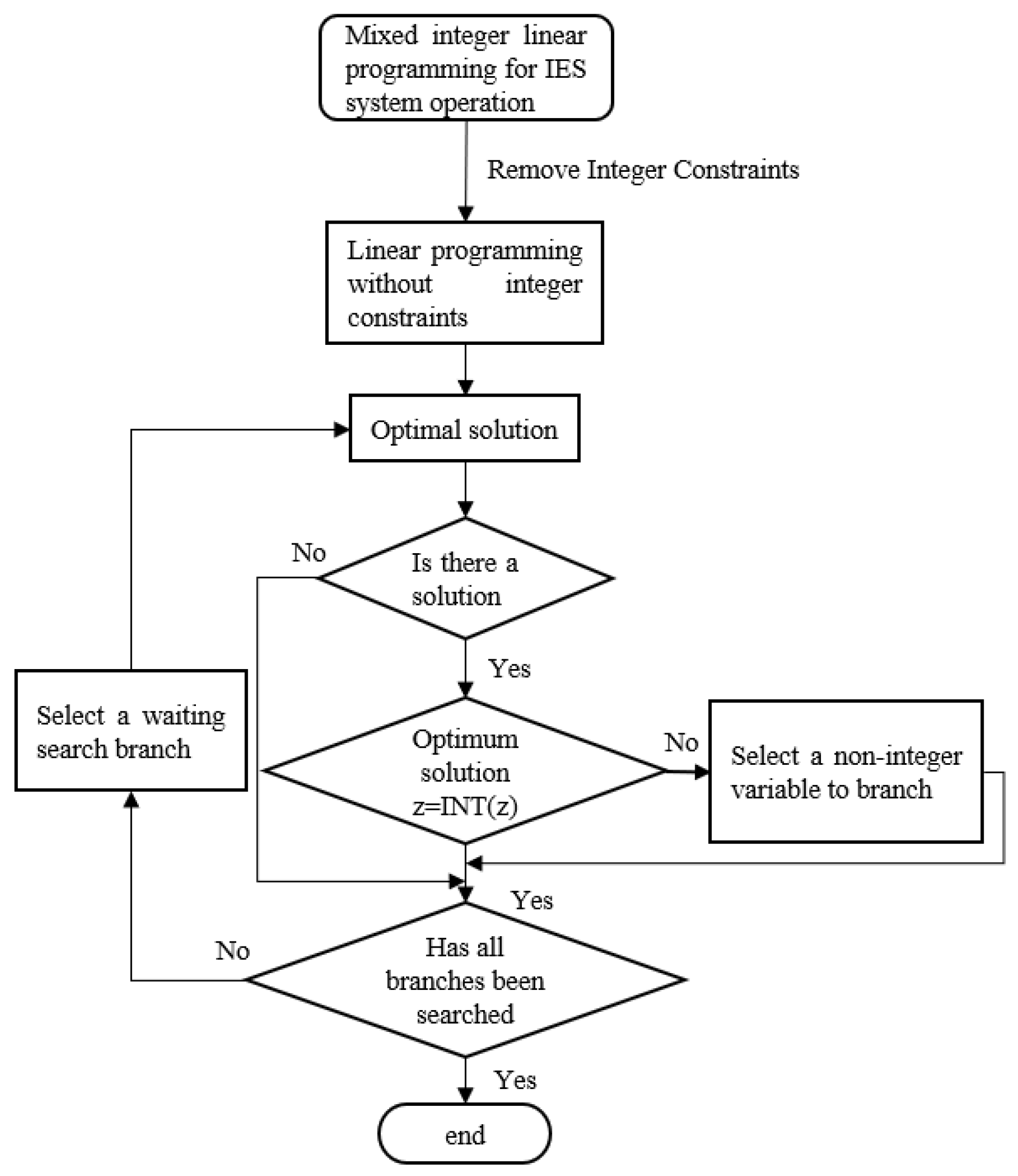
3.3.2. Economic Operation Optimization

To solve the 0–1 mixed integer linear programming problem given for the integrated energy system [29], the branch and bound method is used, and the solving flow chart is illustrated in Figure 5. By removing the integer restriction, the branch and bound technique converts the integer programming problem into a noninteger programming problem and finds the best solution. For those subgroups whose boundaries exceed the known possible solution value, no additional branching is done after each branching. Many subgroups of the solution can be eliminated in this way, narrowing the search. This process is repeated until a feasible solution is identified that has a value that is not greater than the boundaries of any subset, yielding the optimal integer solution.

In this paper, the scheduling method uses time as the scale to schedule the output of each device in distinct time intervals. The scheduling method of the park is determined by monitoring the production of each piece of equipment over the course of 24 h. Firstly, the output of the equipment is examined and the output of the equipment is a real variable. Because the device must operate within a specific power range—with maximum and minimum power constraints—if only real variables are utilized to represent the capability of the device, the output of the device will constantly lie between the lowest and greatest power levels as a result. To put it another way, the device will never stop working. This is in direct conflict with the actual production process’s equipment schedule. The method of adding logical variables is used in this research, with a 0–1 logical variable representing the start and stop states of the device. Real number variables are utilized to describe the equipment’s operating power, and 0–1 variables are used to represent the start and stop states of the equipment, which can thoroughly represent the running state of the equipment in actual production, allowing for scheduling optimization [30].

The scheduling scenario, according to the study, is a predicted analysis of a single equipment’s production throughout the course of 24 h. As a result, there is a real variable representing the running power of the equipment and a 0–1 variable representing the start and stop state of the equipment for the internal combustion engine, lithium bromine refrigerator, centrifugal water cooler, and waste heat recovery device. There is a real variable for cold and thermal energy storage equipment that represents the equipment’s energy storage and emission, and each variable corresponds to 24 h, thus there are 24 values. The park equipment scheduling results are achieved by solving the values of real and logical variables of various equipment.

4. Result and Discussion

The ideal economic dispatch is determined using the usual daily load demand of Wuhan Creative World Park during the winter heating season and summer cooling season. The operating scheduling is examined in light of the park’s equipment conditions. The following are the equipment parameters Figure 6,

Table 2. Multiple energy price parameters.

Parameter name	Value
Natural gas price	2.2 ¥/Nm3
Price of hot and cold energy	0.5557 ¥/kWh
Sell electricity prices	0.7661 ¥/kWh
Power purchase prices	Time-sharing electricity

and

Table 3. System equipment parameters.

Equipment	Value
Thermal efficiency of internal combustion engine	0.52
Refrigeration efficiency of lithium bromide refrigeration unit	0.75
Heating efficiency of lithium bromide refrigeration unit	0.91
Maximum power of gas internal combustion generator	4.044 MW
Maximum refrigeration power of lithium bromide refrigeration unit	3.37 MW
bromide refrigeration unit	3.7 MW
Maximum power of centrifugal refrigerator	3.37 MW
the reserves of tank	450 m3
Charge rate of cold storage tank	1.78 GJ/h
Energy release rate of cold storage tank	3.56 GJ/h
Charge rate of heat storage tank	7.2 GJ/h
Energy release rate of heat storage tank	7.2 GJ/h

.

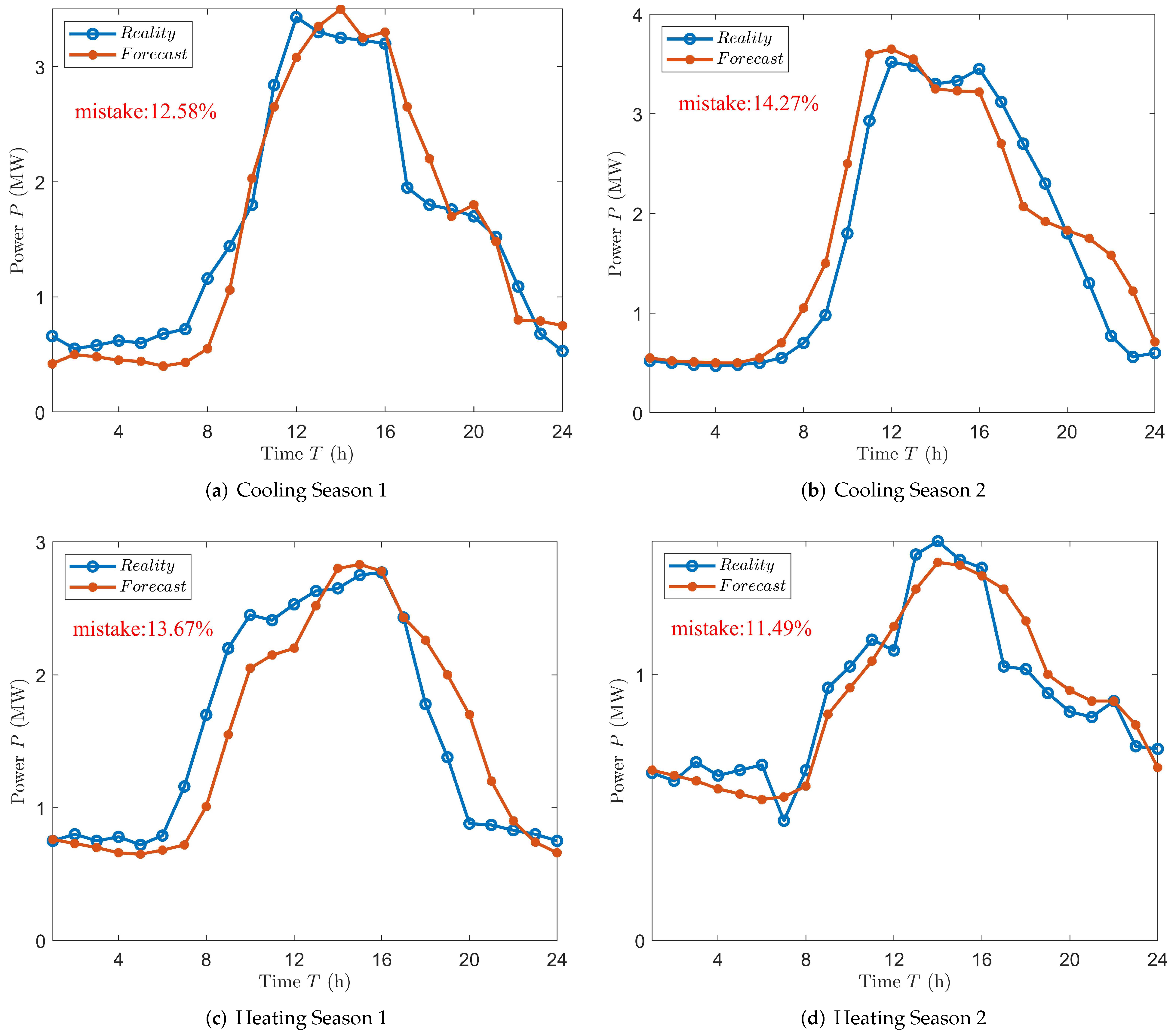
4.1. Mistake Analysis of Neural Network Prediction Algorithm

People typically utilize the strategy of picking average days to anticipate load in an integrated energy system, which is relatively straightforward but has low prediction accuracy. The article [31] Choose one day from the cooling and heating seasons as typical day data for prediction analysis, and assess the entire energy supply season with single-day data, which can only be used as a theoretical reference and cannot be used in real engineering. The article [32] Choose a few typical days for an analysis of a specific energy supply season, and the prediction findings are inaccurate. A suitable typical day technique [33] was chosen for testing in this work, and a typical day was chosen for examination in each month of the energy supply season. The difference between the calculated prediction results and the actual data from the energy station is compared to the artificial neural network technique employed in this study, demonstrating the accuracy and applicability of the current technology. Data from various types of energy supply in various years were chosen at random for analysis. The following Figure 7 shows the findings of the mistake analysis.

The two prediction methods’ prediction outcomes are contrasted and studied. The traditional approach’s mistake varies between 15 and 80 percent, while the prediction method used in this paper’s experiment varies between 10 and 20 percent. The conventional method’s prediction mistake is substantially higher than the artificial neural network prediction method’s, and the traditional method’s fluctuation is also higher. The fundamental reason for this is that the standard method uses average daily data as a baseline and ignores the impact of weather, temperature, and user rate fluctuations on user load. When there is a significant change in user load data over the course of a month, the forecast data will deviate significantly. The forecast method used in this research takes into account the effects of weather, temperature, and usage rate, resulting in a more consistent and accurate prediction than the old method.

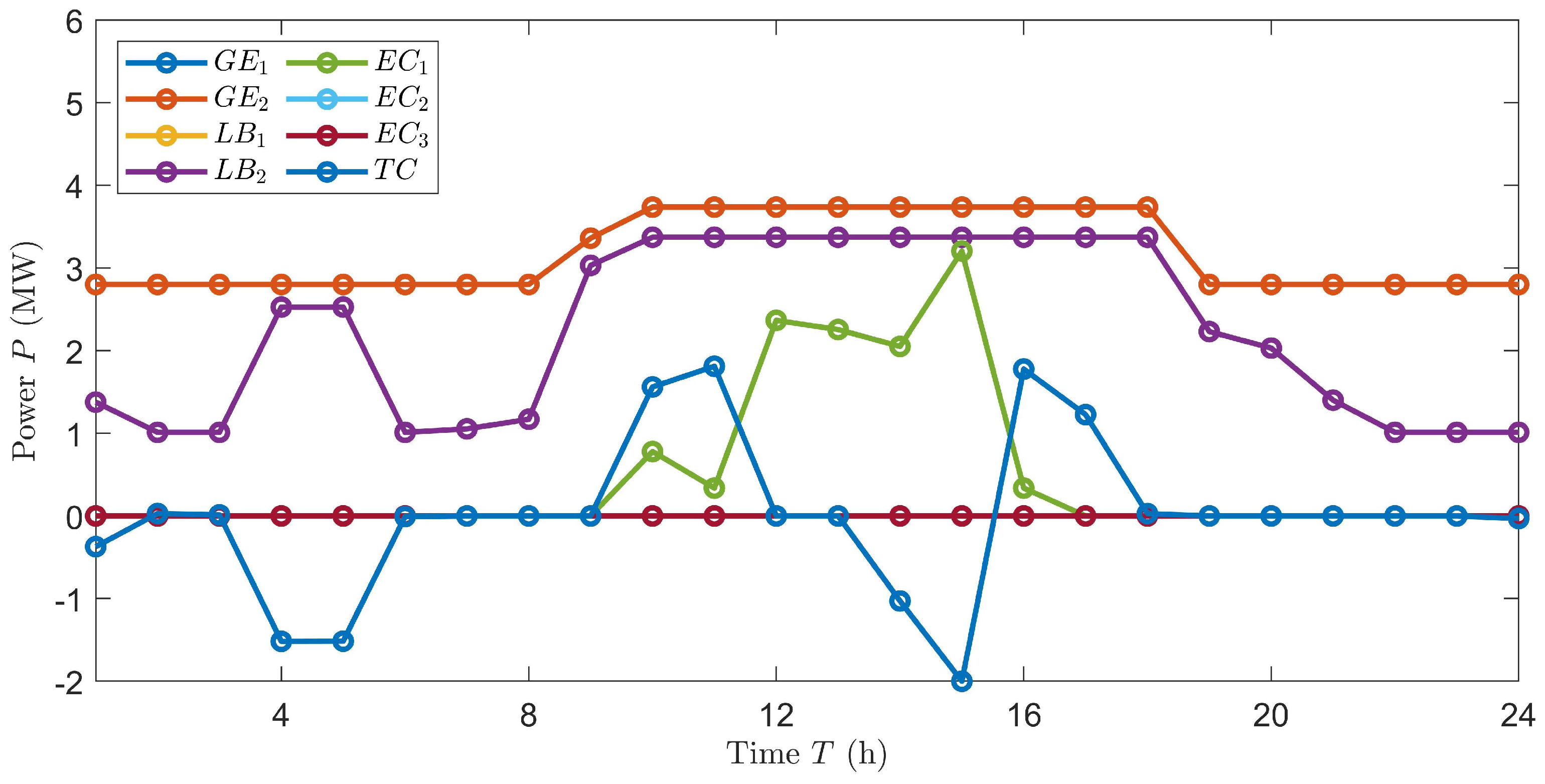
4.2. Economic Operation Optimization in Different Periods

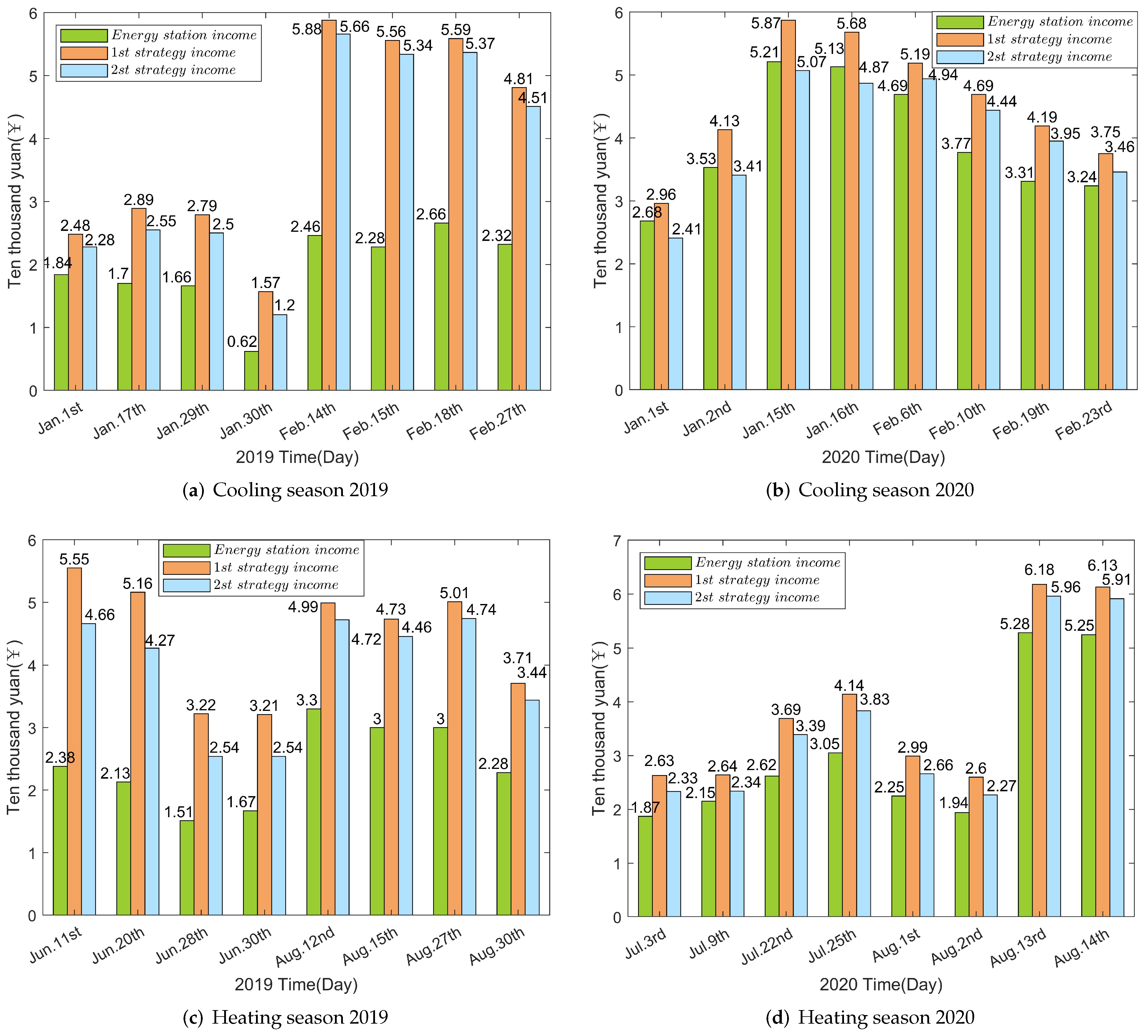
4.2.1. Economic Operation Optimization in Heating Season

The heating season’s economic operation is changed based on time-sharing electricity and natural gas prices. Because the price of natural gas is now low, the internal combustion engine will be run at maximum power to maximize the economic benefits. To plan a lithium bromide refrigeration unit, consider the time-of-use price. When the electricity price is low, it will work from 0 to 7 a.m. and energy storage. The operation is reduced from 8 a.m. to 12 a.m. when the electricity price is high. Bromine machine raises heating power and performs storage from 12 a.m. to 4 p.m. due to increased load and low electricity price. It employs stored thermal energy to provide between 4 and 8 p.m., when electricity prices are at their highest.

Negative denotes the energy charging of the energy storage tank, and regular represents the energy releasing of the energy storage tank, as demonstrated in the image below for the energy curve of the water tank. Using the grid to buy and sell electricity. Negative indicates that you are purchasing electricity from the grid, while positive indicates that you are selling electricity to the system. The current pattern of modifying power prices based on load and electricity price was maintained. The thermal load need of customers is assured first in the thermal determination mode, and the electricity load is delivered according to the producing capacity that fulfills the thermal load demand. The surplus electricity is connected to the grid, while the insufficient power is acquired from the grid Figure 8 and Figure 9.

In the figure, $TC$ represents the power of the water tank, positive represents output, negative represents input; $G{E}_1$ represents the power created by the first internal combustion engine in a day on an hourly basis; $G{E}_2$ represents the second internal combustion engine; $L{B}_1$ represents the first lithium bromide refrigerator’s cooling or heating power per hour per day; $L{B}_2$ represents the second one; $E{C}_1$ represents the first centrifuge’s refrigeration power per hour each day; $E{C}_2$ represents the second one; $E{C}_3$ represents the third one; $Grid$ represents the power of the grid, a positive value indicates that electricity is being sold to the grid, while a negative value indicates that power is being purchased from the grid.

4.2.2. Economic Operation Optimization in Cooling Season

According to the park’s current circumstances, the cooling season’s scheduling was enhanced, and three centrifugal chillers were added to meet the cooling demand caused by the increased user load during the cooling season. The internal combustion engine continues to product electricity, ensuring revenue, due to the low price of natural gas at the time. In the method of determining electricity by heat and determining heat by electricity, the output of the bromine machine and centrifugal water-cooling unit is regulated according to the peak and valley prices of electricity. When the electricity price is low, the cooling capacity is expanded and stored, and when the electricity price is high, the energy storage is used to add cooling, resulting in the economic optimization of the equipment operation. Figure 10 and Figure 11 depicts the equipment’s output.

Because of the higher user load during the cooling season, revenue is slightly higher than during the heating season. Due to the park’s uniqueness, the sale price is higher in both modalities of determining electricity by heat and determining heat by electricity. As a result, selling generated electricity to the grid first might sometimes result in a better economic return, but supplying electricity to users can result in a lower return.

At the same time, the determining electricity by heat mode can meet users’ cold and heat load as well as their electrical load. Users’ demand for cold and hot loads is assured first in this mode, and if power generation is insufficient, they purchase power from the power grid to avoid a power deficit. If electricity is utilized to determine heat, however, there may be insufficient cooling and heating supply, necessitating compensation for some of the consumers lost. As a result, the revenue from determining heat by electricity mode is slightly lower than the revenue from determining electricity by heat mode in this system.

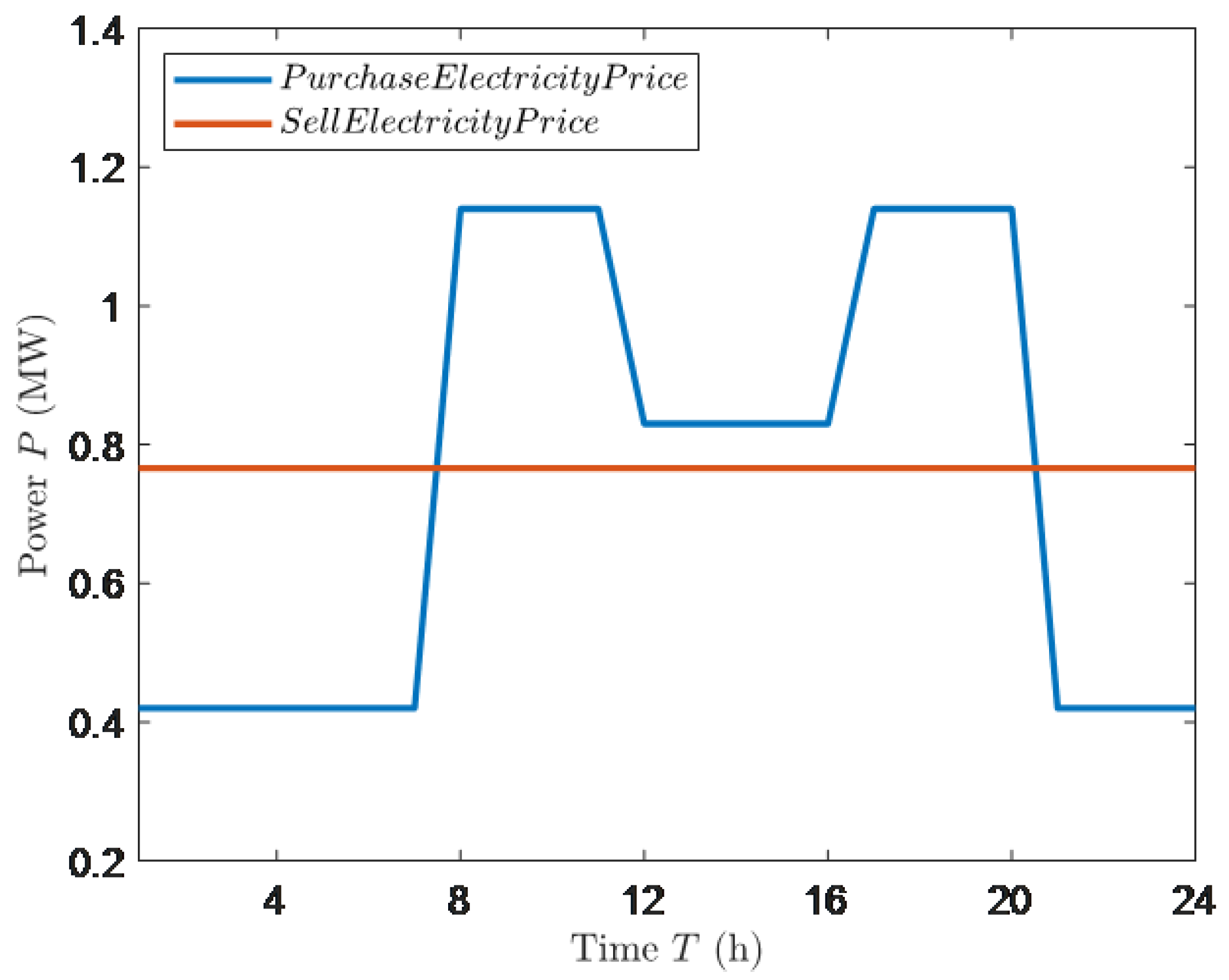
4.3. Operation Optimization for Different Energy Prices

The buy or sale price of various energy, including the purchase price of natural gas and the purchase price of electricity, is a major factor in the economic optimization of the park’s varied equipment. Using the cooling season as an example, this research examines the production of equipment when natural gas prices are low, high, and peak-valley power prices are taken into account, as shown in Figure 12:

When gas prices are low, the park chooses full power generation to maximize economic benefits, as seen in Figure 10 and Figure 12. To guarantee that waste heat is recycled to the greatest extent possible, a lithium bromide unit is employed to absorb refrigeration. Select a part of internal combustion engines to work when natural gas prices are greater. Also, to reduce the use of natural gas, try lowering the internal combustion engine’s operating power. As the power of an internal combustion engine is lowered, so does the amount of high-temperature exhaust smoke produced. When the cooling capacity of the lithium bromide refrigerator is insufficient to suit the needs of the customers, the centrifugal water-cooling unit is activated. A lithium bromide refrigerator and a centrifugal water-cooling unit provide the cooling load. According to the aforesaid optimization approach, this study picks 16 days from data from 2019 and 2020 for a comparison analysis of the optimal operating results and the actual results of the plant, with half of the data from the cooling and another from heating seasons. The Figure 13 depicts the real data and optimization results. At the end of the article, there are detailed data analysis

Table 4. Results of actual running and optimization algorithm running.

Load Type	Data	* Power Ratio	User Load (MWh)	Gas Price ¥/m3	Selling Price of Electricity (¥/kWh)	Load Price (¥/kWh)	Energy Station Income (¥)	* 1st Strategy Income	* 2st Strategy Income
Cooling Load	19.1.11	12.98%	57.02	2.961	0.7076	0.678	18,471	24,847	22,830
Cooling Load	19.1.17	45.44%	63.06	2.961	0.7076	0.678	17,099	28,974	25,508
Cooling Load	19.1.29	94.98%	63.2	2.961	0.7076	0.678	16,648	27,922	25,046
Cooling Load	19.1.30	97.58%	35.74	2.961	0.7076	0.678	6214	15,729	12,075
Cooling Load	19.2.14	27.62%	110	2.961	0.7076	0.678	24,695	58,819	56,616
Cooling Load	19.2.15	24.43%	104	2.961	0.7076	0.678	22,801	55,617	53,415
Cooling Load	19.2.18	69.07%	105	2.961	0.7076	0.678	26,695	55,943	53,740
Cooling Load	19.2.27	54.98%	88.74	2.961	0.7076	0.678	23,215	48,154	45,120
Heating Load	19.6.11	78.76%	100	2.961	0.7076	0.678	23,871	55,504	46,672
Heating Load	19.6.20	72.48%	94.62	2.961	0.7076	0.678	21,386	51,621	42,789
Heating Load	19.6.28	43.49%	64.26	2.961	0.7076	0.678	15,157	32,217	25,408
Heating Load	19.6.30	44.14%	69.38	2.961	0.7076	0.678	16,771	32,117	25,488
Heating Load	19.8.12	45.68%	90	2.961	0.7076	0.678	33,027	49,979	47,222
Heating Load	19.8.15	43.73%	85.28	2.961	0.7076	0.678	30,001	47,366	44,609
Heating Load	19.8.27	37.02%	90.35	2.961	0.7076	0.678	30,069	50,172	47,416
Heating Load	19.8.30	37.02%	66.91	2.961	0.7076	0.678	22,839	37,198	34,441
Cooling Load	20.1.1	32.46%	47.6	2.713	0.7076	0.644	26,866	29,666	24,174
Cooling Load	20.1.2	45.46%	65.52	2.713	0.7076	0.644	35,317	41,312	34,133
Cooling Load	20.1.15	68.59%	93.14	2.713	0.7076	0.644	52,132	58,769	50,739
Cooling Load	20.1.16	69.02%	90.75	2.713	0.7076	0.644	51,384	56,827	48,797
Cooling Load	20.2.6	59.74%	96.48	2.713	0.7076	0.644	46,911	51,970	49,490
Cooling Load	20.2.10	63.6 %	87.56	2.713	0.7076	0.644	37,776	46,939	44,459
Cooling Load	20.2.19	56.9 %	78.45	2.713	0.7076	0.644	33,142	41,992	39,512
Cooling Load	20.2.23	46.75%	59.66	2.713	0.7076	0.644	32,489	37,534	34,638
Heating Load	20.7.3	92.23%	46.83	2.313	0.678	0.554	18,795	26,370	23,335
Heating Load	20.7.9	91.79%	47	2.313	0.678	0.554	21,507	26,464	23,430
Heating Load	20.7.22	78.8 %	66	2.313	0.678	0.554	26,297	36,975	33,941
Heating Load	20.7.25	77.94%	74	2.313	0.678	0.554	30,517	41,402	38,368
Heating Load	20.8.1	12.98%	54.42	2.313	0.678	0.554	22,547	29,958	26,647
Heating Load	20.8.2	24.24%	47.88	2.313	0.678	0.554	19,413	26,057	22,745
Heating Load	20.8.13	99.32%	115.48	2.313	0.678	0.554	52,843	61,896	59,693
Heating Load	20.8.14	98.88%	114.59	2.313	0.678	0.554	52,511	61,352	59,149

* Power ratio: Actual generating capacity as a percentage of total generating capacity; * 1st strategy: determining electricity by heat; * 2st strategy: determining heat by electricity.

.

According to the above figure, the energy station’s major revenue comes from selling electricity and cooling and heating loads, while the main cost comes from natural gas use. As a result, too much generation during the 2019 cooling and heating seasons, when gas prices are higher, could result in reduced income. On 30 January 2019, for example, the user load was low, resulting in lower cooling and heat load revenue. Meanwhile, the gas internal combustion engine was set to work at nearly full capacity, resulting in more electrical generation and higher losses, ultimately ending in a day of a very low revenue. The power of gas internal combustion engines can be enhanced correctly to increase revenue due to the lower price of natural gas in the 2020 heating season. As indicated in the table, the energy station’s revenue has climbed considerably this season. For the 2020 cooling season, natural gas prices are continue to plummet. Electricity prices have declined, but at a slower rate than natural gas prices. As a result, choosing natural gas to run at a greater power level at this time would be more profitable, as evidenced by the comparison between 2 August and 13 August.

The operation of the energy station is not totally suitable, according to historical data, and at times, the comprehensive electricity price, natural gas price, and the greatest profit that the user load can accomplish are not taken into account. As a result, the following analysis results can be achieved by substituting the forecast data into the optimization method for analysis. The optimization algorithm may generate larger economic income under the same user load because it fully considers the price of various links and analyzes the demand of users. At the same time, as previously said, determining electricity by heat mode can undoubtedly fulfill user demand for cooling and heating load, but determining heat by electricity may not be able to meet user demand for cooling and heating load. As a result, certain user losses must be compensated, and the determining heat by electricity mode’s profit is lower than determining electricity by heat mode. This is also why the revenue of the electricity-fixed heat mode in the chart for the cooling season of 2020 is lower than the real operation condition. It is because the customer has a high-load demand but less power generation, resulting in less high-temperature smoke and less refrigeration. As a result, the user’s cooling load need cannot be supplied, and compensation is required. When comparing the cooling seasons of 2020 and 2019, the proportion of economic advantages after the optimized operation in 2019 is higher, and both the optimization and the real operation appear to have an amplitude of economic benefits. Because user load and electricity generation have upper limits, it is hard to continuously improve economic benefits. In 2019, when petrol prices are high, the park has a lot of space for improvement. When natural gas prices were low in 2020, the park decided to run the internal combustion engine at full capacity, which was consistent with optimization theory. As a result, there is still opportunity for development in 2019.

According to the results of the aforesaid data analysis, the optimized operation scheme provided in this work has larger economic benefits and is better than the traditional scheduling approach when compared to the actual operating condition. Two scheduling methods are utilized in the system’s optimal scheduling strategy to determine the electricity by heat and the heat by electricity. The two scheduling approaches have some improvements when compared to the real operation of the system, with the control strategy based on determining the electricity by heat being more lucrative and suitable for the park’s actual operation.

5. Conclusions

This paper presents a day-ahead optimal scheduling method for integrated energy systems that incorporates an accurate prediction model and multiple energy storage types and analyzes it by incorporating an accurate prediction model and multiple energy storage models into common economic operation strategies. The 0–1 mixed integer linear programming issue was solved using the branch-and-bound method. Finally, an optimization experiment was carried out using real data from a Wuhan park. The case study reveals that establishing an accurate prediction model may enhance forecast accuracy by around 10%, and the revenue optimization outcome is considerably better than the park’s real operation revenue, which is at least 10.45% higher. Finally, when compared to that of the traditional method, this method is more practical and feasible, and it can be implemented in a real integrated energy system.

References

1. Muhammad Fahad, Z.; Elhoussin, E.; Mohamed, B. Microgrids energy management systems: A critical review on methods, solutions, and prospects. Appl. Energy 2018, 222, 1033–1055. [Google Scholar]
2. Xiao, H.; Heng, Z. Multi-objective planning for integrated energy systems considering both exergy efficiency and economy. Energy 2020, 197, 117155. [Google Scholar]
3. Li, F.; Lu, S.; Cao, C.; Feng, J. Operation Optimization of Regional Integrated Energy System Considering the Responsibility of Renewable Energy Consumption and Carbon Emission Trading. Electronics 2021, 10, 2677. [Google Scholar] [CrossRef]
4. Squalli, J. Renewable energy, coal as a baseload power source, and greenhouse gas emissions: Evidence from U.S. state-level data. Energy 2017, 127, 479–488. [Google Scholar] [CrossRef]
5. Bagherian, A.; Mehranzamir, K. Classification and Analysis of Optimization Techniques for Integrated Energy Systems Utilizing Renewable Energy Sources: A Review for CHP and CCHP Systems. Processes 2021, 9, 339. [Google Scholar] [CrossRef]
6. Ziqi, L.; Junjie, Y. Research on Optimized Energy Scheduling of Rural Microgrid. Appl. Sci. 2020, 9, 4641. [Google Scholar]
7. Dawn, S.; Gope, S.; Das, S.S.; Ustun, T.S. Social Welfare Maximization of Competitive Congested Power Market Considering Wind Farm and Pumped Hydroelectric Storage System. Electronics 2021, 10, 2611. [Google Scholar] [CrossRef]
8. Xiaohui, Y.; Zaixing, C.; Xin, H. Robust capacity optimization methods for integrated energy systems considering demand response and thermal comfort. Energy 2021, 221, 119727. [Google Scholar]
9. Pan, G.; Gu, W.; Lu, Y.; Qiu, H.; Lu, S.; Yao, S. Optimal Planning for Electricity-Hydrogen Integrated Energy System Considering Power to Hydrogen and Heat and Seasonal Storage. IEEE Trans. Sustain. Energy 2020, 11, 2662–2676. [Google Scholar] [CrossRef]
10. Yuman, Z.; Xuezhi, L.; Zheng, Y. Decomposition-coordination based optimization for PV-BESS-CHP integrated energy systems. Trans. China Electrotech. Soc. 2020, 35, 2372–2386. [Google Scholar]
11. Liu, C.; Shahidehpour, M.; Wang, J. Coordinated scheduling of electricity and natural gas infrastructures with a transient model for natural gas flow. Chaos 2011, 21, 531. [Google Scholar] [CrossRef] [PubMed]
12. Martins, J.; Spataru, S.; Sera, D. Comparative Study of Ramp-Rate Control Algorithms for PV with Energy Storage Systems. Energies 2019, 12, 1342. [Google Scholar] [CrossRef] [Green Version]
13. Zhang, L.; Kuang, J.; Sun, B.; Li, F.; Zhang, C. A two-stage operation optimization method of integrated energy systems with demand response and energy storage. Energy 2020, 208, 118423. [Google Scholar] [CrossRef]
14. Li, Y.; Han, M.; Yang, Z.; Li, G. Coordinating Flexible Demand Response and Renewable Uncertainties for Scheduling of Community Integrated Energy Systems with an Electric Vehicle Charging Station: A Bi-Level Approach. IEEE Trans. Sustain. Energy 2021, 12, 2321–2331. [Google Scholar] [CrossRef]
15. Guoqing, L.; Rufeng, Z.; Tao, J. Optimal dispatch strategy for integrated energy systems with CCHP and wind power. Appl. Energy 2017, 192, 408–419. [Google Scholar]
16. Yongli, W.; Yuze, M.; Fuhao, S.; Yang, M. Economic and efficient multi-objective operation optimization of integrated energy system considering electro-thermal demand response. Energy 2020, 205, 118022. [Google Scholar]
17. Xianchao, L.; Yi, D. Energy management of CCHP microgrid considering demand-side management. In Proceedings of the 2017 32nd Youth Academic Annual Conference of Chinese Association of Automation (YAC), Hefei, China, 19–21 May 2017; pp. 240–245. [Google Scholar]
18. Xijun, G.; Ling, W. Optimal Cooperative Scheduling in Multienergy Micro-grid Considering Demand Response. In Proceedings of the 2019 IEEE 3rd International Electrical and Energy Conference (CIEEC), Beijing, China, 7–9 September 2019; pp. 1997–2002. [Google Scholar]
19. Canhuang, Z.; Huansheng, Z. Optimal Capacity Design for Solar-assisted CCHP System Integrated with Energy Storage. In Proceedings of the 2019 IEEE PES GTD Grand International Conference and Exposition Asia (GTD Asia), Bangkok, Thailand, 19–23 March 2019; pp. 691–696. [Google Scholar]
20. Qinghua, W.; Jizhen, L. Optimal Operation Strategy of Multi-Energy Complementary Distributed CCHP System and its Application on Commercial Building. IEEE Access 2019, 7, 127839–127849. [Google Scholar]
21. Jinxia, L.; Shouzhen, Z. Combined economic operation research of CCHP system and energy storage. In Proceedings of the 2014 International Conference on Information Science, Electronics and Electrical Engineering, Sapporo, Japan, 26–28 April 2014; pp. 574–578. [Google Scholar]
22. Rui, Z.; Jianyong, Z. Economical Optimal Operation of Multienergy System Considering Uncertainty. In Proceedings of the 2018 IEEE 3rd Advanced Information Technology, Electronic and Automation Control Conference (IAEAC), Chongqing, China, 12–14 October 2018; pp. 447–452. [Google Scholar]
23. Verwiebe, P.A.; Seim, S.; Burges, S. Modeling Energy Demand—A Systematic Literature Review. Energies 2021, 14, 7859. [Google Scholar] [CrossRef]
24. Kim, G.; Hur, J. A Short-Term Power Output Forecasting Based on Augmented Naïve Bayes Classifiers for High Wind Power Penetrations. Sustainability 2021, 13, 12723. [Google Scholar] [CrossRef]
25. Al-Zadjali, S.; Al Maashri, A.; Al-Hinai, A. A Fast and Accurate Wind Speed and Direction Nowcasting Model for Renewable Energy Management Systems. Energies 2021, 14, 7878. [Google Scholar] [CrossRef]
26. Singh, S.; Chauhan, P.; Aftab, M.A. Cost Optimization of a Stand-Alone Hybrid Energy System with Fuel Cell and PV. Energies 2020, 13, 1295. [Google Scholar] [CrossRef] [Green Version]
27. Dhifli, M.; Lashab, A.; Guerrero, J.M.; Abusorrah, A.; Al-Turki, Y.A.; Cherif, A. Abusorrah. Enhanced Intelligent Energy Management System for a Renewable Energy-Based AC Microgrid. Energies 2020, 13, 3268. [Google Scholar] [CrossRef]
28. Huang, S.; Fang, L. Summary of Micro-grid Economic Optimization Operation. In Proceedings of the 2019 IEEE Sustainable Power and Energy Conference (iSPEC), Beijing, China, 21–23 November 2019; pp. 305–311. [Google Scholar]
29. Zhengyi, L.; Zhaoyi, H. Optimization and Analysis of Operation Strategies for Combined Cooling, Heating and Power System. In Proceedings of the 2011 Asia-Pacific Power and Energy Engineering Conference, Wuhan, China, 25–28 March 2011; pp. 1–4. [Google Scholar]
30. Masatoshi, S.; Kosuke, K. Operational Planning of District Heating and Cooling Plants through Genetic Algorithms for Mixed 0–1 Linear Programming. Eur. J. Oper. Res. 2002, 137, 677–687. [Google Scholar]
31. Jian, G.; Dongmei, Y. Optimized operation of a distributed integrated energy microgrid for cogeneration of cold, heat and electricity with energy storage. Electr. Power Eng. Technol. 2021, 125, 25–32. [Google Scholar]
32. Zhao, H.; Lu, H.; Wang, X.; Li, B.; Wang, Y.; Liu, P.; Ma, Z. Research on Comprehensive Value of Electrical Energy Storage in CCHP Microgrid with Renewable Energy Based on Robust Optimization. Energies 2020, 13, 6526. [Google Scholar] [CrossRef]
33. Beihong, Z.; Weiding, L. Optimal unit sizing of combined cooling heating and power systems. Heat. Vent. Air Cond. 2005, 35, 4. [Google Scholar]
Figure 1. System block diagram.
Electronics 11 00022 g001
Figure 2. Energy flow diagram of system.
Electronics 11 00022 g002
Figure 3. Model testing for training.
Electronics 11 00022 g003
Figure 4. Load prediction results.
Electronics 11 00022 g004
Figure 5. Branch and bound algorithm flow chart.
Electronics 11 00022 g005
Figure 6. Price of buying or selling electricity.
Electronics 11 00022 g006
Figure 7. Mistake analysis of prediction algorithm.
Electronics 11 00022 g007
Figure 8. Equipment output (heating season, determining electricity by heat).
Electronics 11 00022 g008
Figure 9. Equipment output (heating season, determining heat by electricity).
Electronics 11 00022 g009
Figure 10. Equipment output (cooling season, determining electricity by heat).
Electronics 11 00022 g010
Figure 11. Equipment output (cooling season, determining heat by electricity).
Electronics 11 00022 g011
Figure 12. Operation of equipment in cooling season (high gas price).
Electronics 11 00022 g012
Figure 13. Scheduling optimization results comparison.
Electronics 11 00022 g013