Human-Machine Cooperative Trajectory Planning for Semi-Autonomous Driving Based on the Understanding of Behavioral Semantics

Abstract

This paper presents a novel cooperative trajectory planning approach for semi-autonomous driving. The machine interacts with the driver at the decision level and the trajectory generation level. To minimize conflicts between the machine and the human, the trajectory planning problem is decomposed into a high-level behavior decision-making problem and a low-level trajectory planning problem. The approach infers the driver’s behavioral semantics according to the driving context and the driver’s input. The trajectories are generated based on the behavioral semantics and driver’s input. The feasibility of the proposed approach is validated by real vehicle experiments. The results prove that the proposed human–machine cooperative trajectory planning approach can successfully help the driver to avoid collisions while respecting the driver’s behavior.

1. Introduction

Intelligent driving systems can improve safety and reduce traffic accidents effectively. The current intelligent assistance systems mainly include lane departure warning systems, lane-keeping systems, automatic cruise systems, automatic emergency braking systems, etc. However, the current intelligent driving systems still have many limitations and face many challenges in environmental understanding, decision, planning, and control. In these systems, the allocation mechanism of driving authority between human and machine is relatively simple, and a safe and flexible human–machine cooperative driving ability in a complex environment is not yet available. Drivers and intelligent driving systems can be complementary. Drivers have rich experience and common sense in terms of environmental understanding and cognition. Intelligent driving systems have the ability to continuously monitor the surrounding environment and can assist one in driving safely to reduce the driver’s workload. The advanced stage of human–machine co-driving should be that the driver can get involved in all levels of perception, reasoning, decision making, and control. The advantages of a human driver and intelligent driving system should be integrated to achieve harmonization. How to integrate the advantages of drivers and intelligent driving systems through human–machine co-driving technology has become an important research topic of intelligent driving technology.

Regarding on the handover of driving authority between driver and vehicle in the driver assistance systems, the research mainly includes the scope of application of driving assistance systems [1], the human factors [2], the driving capability of the driver [3], and the authority interactions between the driving assistance system and driver [4]. The effect of an authority transition from autonomous driving mode to driver take-over mode varies with different drivers [5]. It is necessary to analyze the timing to switch the control authority between the driver and the driver assistance system [6]. It is necessary to judge whether the control authority can be transferred safely, whether the driver has the ability to control the vehicle safely, and whether the vehicle state will be in the controllable state-space after the control authority is switched. Differently from control authority switching, adjustable autonomy can set multiple levels of autonomy, and each level can set a different control ratio [7,8]. The driver and the machine can control the velocity and steer separately or together. According to the evaluation criteria, a certain level of autonomy can be selected [9]. The disadvantage of this method is that the autonomy level is divided into several fixed levels, which have poor flexibility. The control of the human and the machine is simply added, since the human’s input is not fixed, the final effect is unpredictable. Some scholars proposed to use a new human–machine interaction interface to solve the problem of control authority interaction. One approach is the haptic shared control, in which both the driver and the intelligent driving system have authority over vehicle control. The driver is in the control loop all the time, and can actively respond to any scene. At the same time, the driver can continuously receive the haptic feedback provided by the intelligent driving system. Human–machine cooperative longitudinal control can be realized by using the accelerator pedal and the brake pedal [10,11]; human–machine cooperative lateral control can be realized by the steering wheel. Haptic shared control can be achieved through force feedback or stiffness feedback, thereby allowing a smooth transfer of control authority between the driver and the machine [12]. Sterling J. Anderson [13] used a method based on model predictive control to design a smooth proportional distribution relationship of human–machine control authority. When the risk reaches a certain level, the control authority will be gradually transferred from human to machine. Manabu et al. [14] proposed a weighted summation method to combine the driver’s input with the automation’s desired input. In this work, the authority weights are static during driving, which does not allow the driver to gain more control authority in a critical situation that cannot be properly handled by automation. Most of the above research focused on the problem of vehicle control when the path is predefined. Few research have discussed the problem of trajectory planning for semi-autonomous driving.

This paper discusses semi-autonomous driving technology from the perspective of trajectory planning. A lot of research has been done on trajectory planning for automated driving. Some approaches focus on computing collision-free trajectories using graph-search methods, such as A* [15], Hybrid A* [16], D* [17], and state-lattice [18]. A disadvantage of graph-search methods is that their results are related to the degree of discretization of sampling points or primitives. If the discretization is not fine enough, the method may not find a feasible path. Aiming at solving the above problem, incremental search methods are proposed, such as Expansive Spaces Tree (EST) [19], Rapidly-exploring Random Trees (RRT) [20], and Stable Sparse Trees (SST) [21]. If there exists a path and given enough time, the incremental search methods will find a feasible path. The graph-search methods and the incremental search methods are suitable for generating paths in an unknown static environment. They usually require too many computing resources, making them unable to react quickly in dynamic scenarios. The numerical optimization methods are often used to obtain smooth trajectories by minimizing or maximizing a cost function. In the artificial potential field methods, obstacles are assigned repulsive forces and the target zone is assigned attractive forces so that the vehicle can drive towards the goal zone while keeping away from the obstacles [22]. The trajectory with the deepest gradient can be chosen as the optimal result. Whereas, the artificial potential field methods face the problem of falling into local minima. Additionally, it is hard to reflect the non-holonomic characteristic of the vehicle. In order to overcome the disadvantages, there are some studies using sampling-based trajectory generation methods, such as polynomial spline [23,24,25]. The polynomial methods can generate paths with curvature bound constraints, and obtain suboptimal solutions in the discrete solution space considering the distance to obstacles and the costs of vehicle movement. One of the advantages of the polynomial methods is that the computational cost is relatively small, and the convergence can be guaranteed.

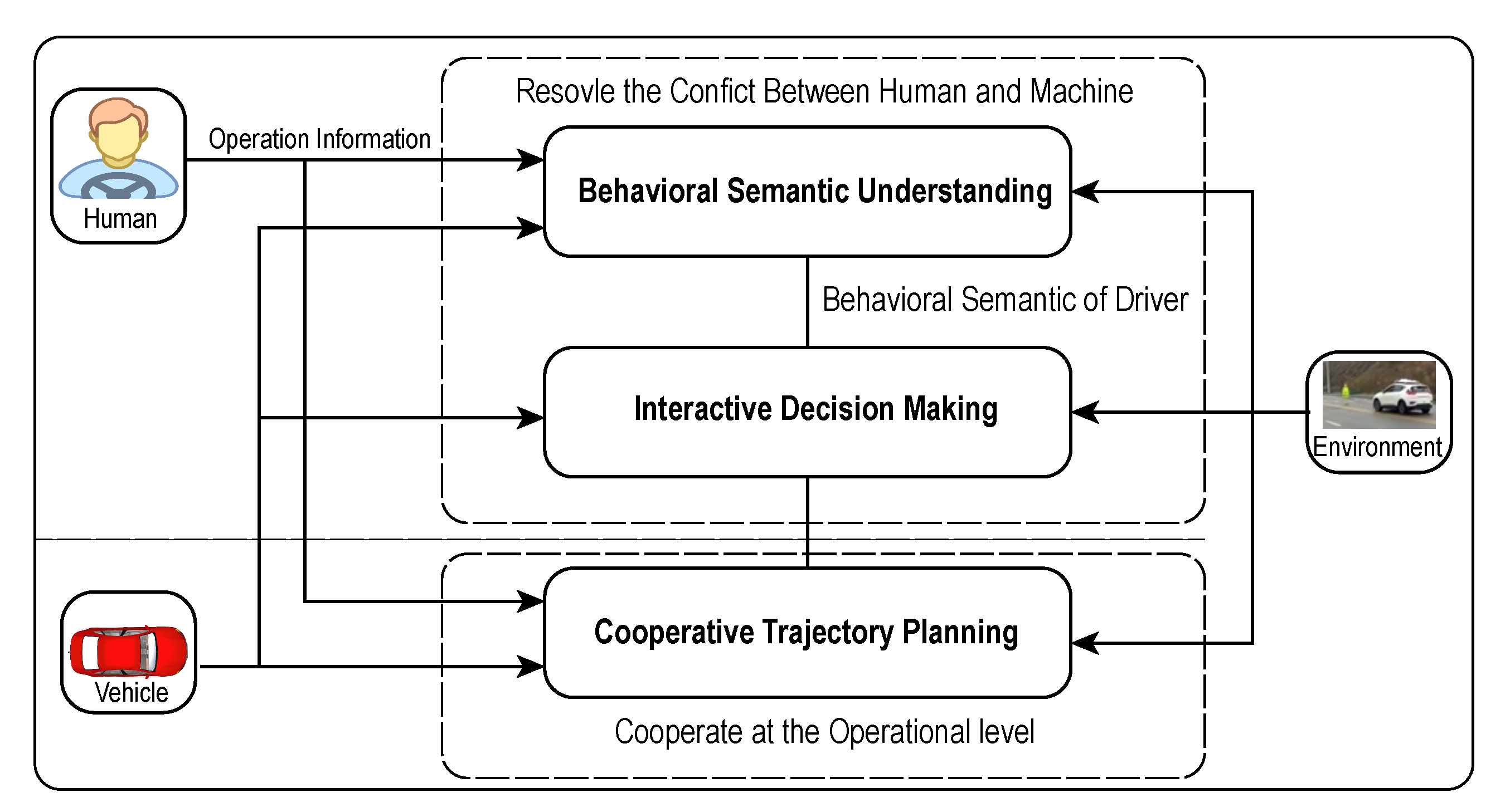
In this paper, we study the situation where the system detects a dangerous situation and assists the driver in avoiding collisions with detected obstacles. In order to reduce the system’s intervention during normal driving, the system enters the semi-autonomous driving mode only when the system detects a dangerous situation. In order to solve the problem of the fusion of driver’s input and machine’s input at the decision level and the operational level, a human–machine collaborative trajectory planning algorithm is proposed that combines the driving behavior and the comprehensive information of the human, vehicle, and road. We adopted the hierarchical planning approach to construct our cooperative trajectory planner. The semi-autonomous driving system respects the driver’s driving behavior at the decision level and driver’s input at the operational level while planning the trajectory. The framework of the proposed approach is shown in Figure 1.

The main contribution of this paper is that the proposed algorithm can perform trajectory planning in a human–machine collaborative manner while respecting the behavioral semantics and the input of the driver. The system interacts with the driver at both the decision level and the trajectory generation level. In addition, the proposed cooperative trajectory planning algorithm can generate trajectories for each specific driving maneuver. The computational cost can be reduced by generating fewer trajectories.

The remainder of this paper is organized as follows. Aiming at reducing conflicts between the driver and the semi-autonomous driving system, the algorithm reasons about the behavioral semantics of the current situation in Section 2. Then the algorithm makes collision avoidance decisions according to the behavioral semantic of the driver in Section 3. In Section 4, the human–machine cooperative trajectory planning algorithm considering the driver’s input is proposed. Section 5 shows the experiment results. Conclusions are drawn in Section 6.

2. Behavioral Semantic Understanding

The rider–horse metaphor (or H-metaphor) describes a symbiotic system, in which the rider controls the horse through a combination of continuous and discrete inputs from the hand to the rein. The horse can understand human intentions through the reins, and the rider can understand the horse’s intentions from the environment and the state of motion [26]. The horse strives to reduce the human’s riding burdens according to the human’s intentions. Similarly, the intelligent assistance system and the human are two dependent agents in a symbiotic system. The intelligent assistance system should understand the driver’s behavioral semantic to resolve the conflicts between human and machine, and strive to fulfil the driver’s intention if the intention is safe.

Driving maneuvering is very much dependent on its context. Each series of actions that a driver can take corresponds to a maneuver, such as lane-keeping, a lane-change, a left turn, or a right turn. Most current papers about semi-autonomous driving track a given path, and the input of the driver is treated as a disturbance, and the machine compensates for the driver’s input. In order to achieve flexible interactions between people and machines, the human–machine co-driving system should have the ability to reason about vehicle movement trends based on behavioral semantics to identify whether the driving behavior is safe or not. The driver can inform the intelligent driving system of lane-changing intentions through the turning signal. Otherwise, the assistance system can understand the behavioral semantics of the driver according to the driver’s driving operation, environment, and vehicle status.

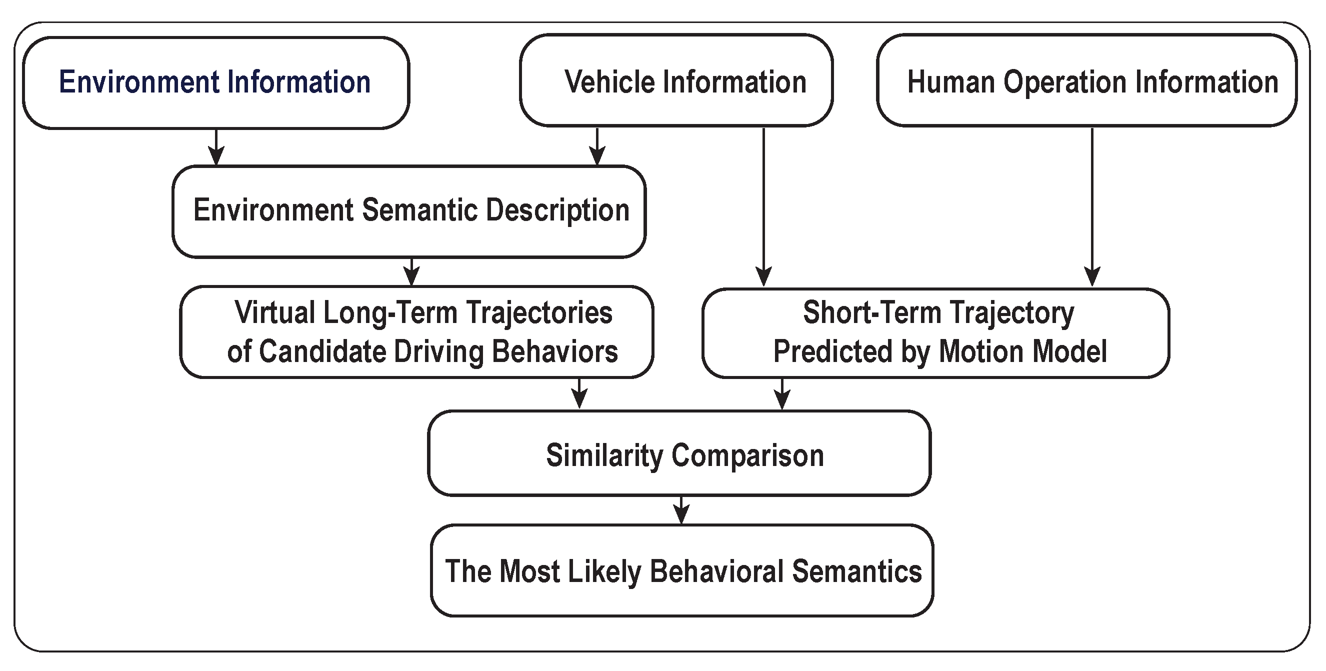
In this paper, we propose a method for understanding the driver’s behavior at the semantic level according to the operation command of the driver and the environmental information. The framework for the behavioral semantic understanding algorithm is shown in Figure 2.

There are three main steps for determining the driver’s most likely behavioral semantics.

Firstly, the virtual trajectories corresponding to specific semantic behaviors are generated. According to the traffic scenario, the vehicle movement is decomposed into lateral movement and longitudinal movement in the $Fren\acute{e}t$-$Frame$.

Secondly, according to the driver’s input, the short-term trajectory is obtained using the constant turn rate and acceleration (CTRA) kinematics motion model.

Finally, the driver’s most likely behavioral semantics is obtained by computing the similarity between the virtual trajectories of different behavioral semantics and the predicted trajectory.

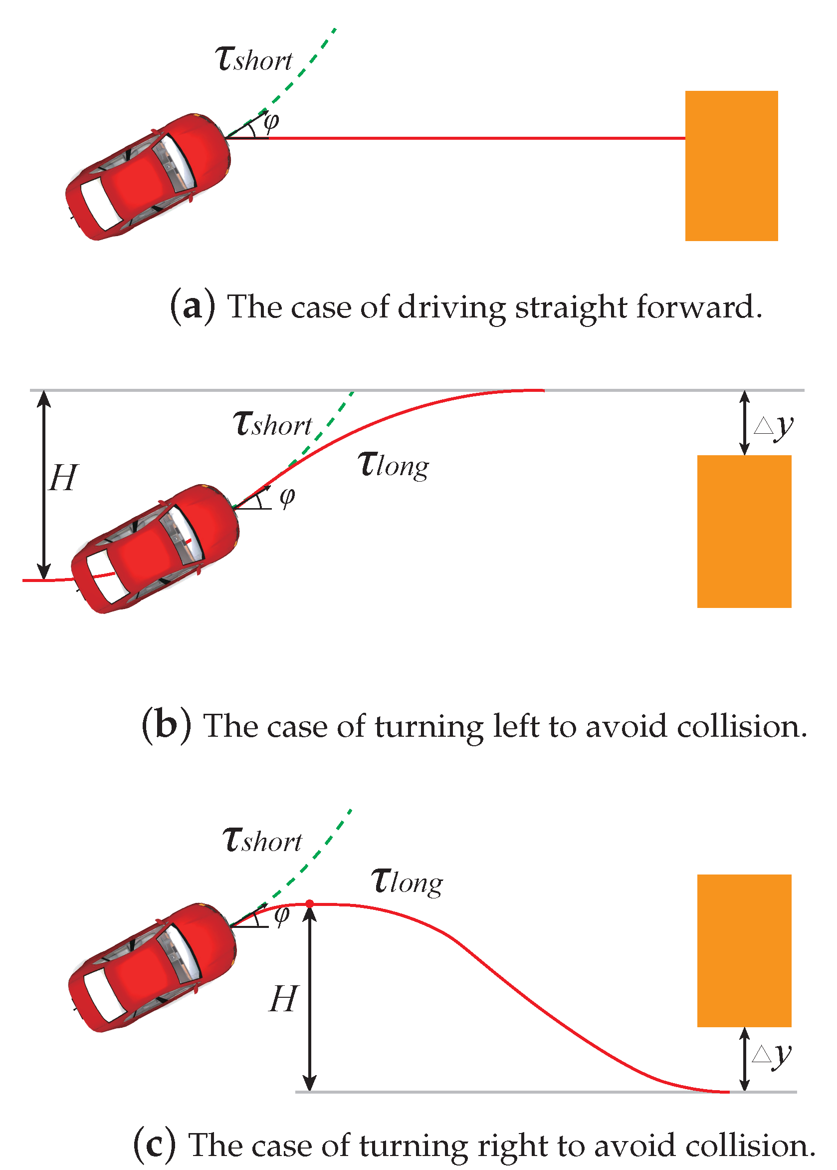
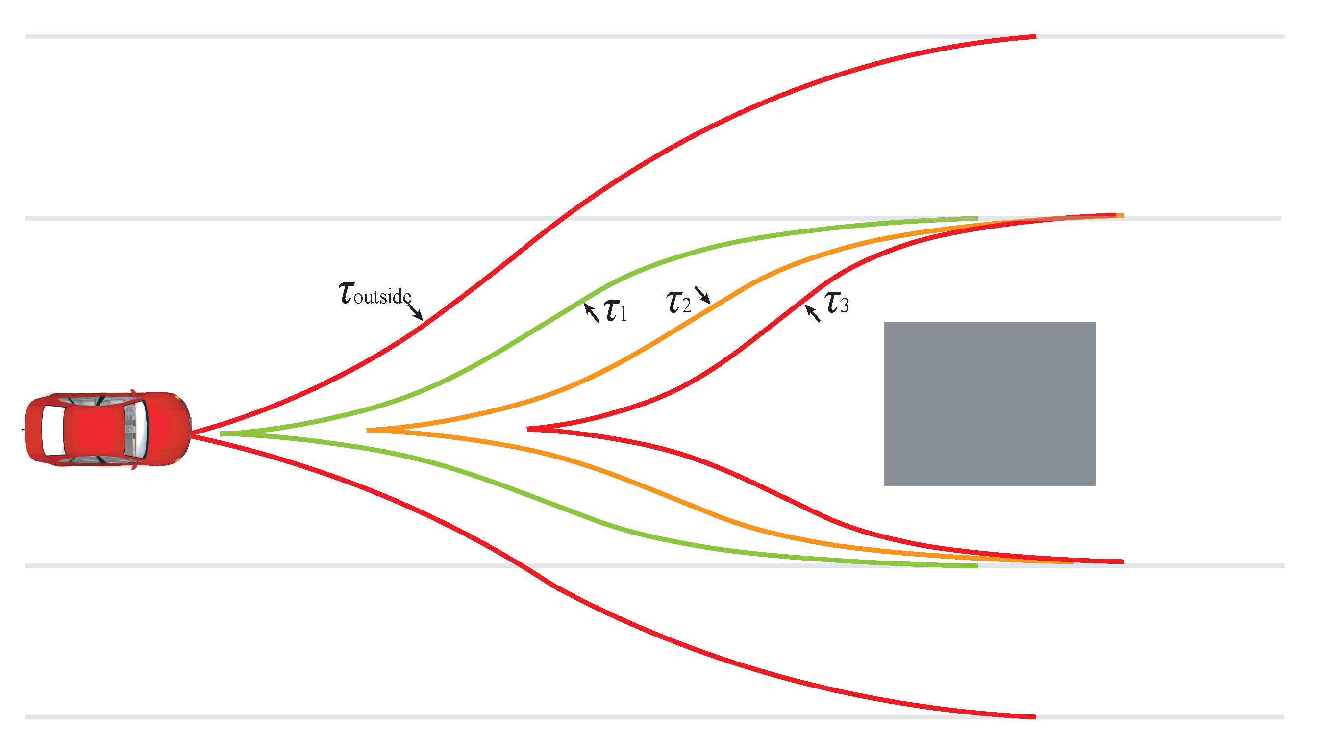
The virtual long-term trajectory of candidate driving behaviors and the short-term predicted trajectory are shown in Figure 3. The trajectory ${\tau }_{long}$ is long-term trajectory of a candidate driving behavior. The trajectory ${\tau }_{short}$ is the short-term predicted trajectory.

2.1. The Virtual Long-Term Trajectories of Candidate Driving Maneuvers

In this paper, in order to reason about the behavioral semantics, the long-term trajectories representing candidate driving maneuvers are generated. An evasive motion model is used in which the lateral acceleration is assumed to be a sinusoidal function of time.

$$\begin{array}{cc}\hfill a_{lat}=& \frac{2\pi H}{t_{lat}^2}sin\left(\frac{2\pi }{t_{lat}}\right)\hfill \end{array}$$

(1a)

$$\begin{array}{cc}\hfill y\left(t\right)=& -\frac{H}{2\pi }sin\left(\frac{2\pi }{t_{lat}}t\right)+\frac{H}{t_{lat}}t+y_0\hfill \end{array}$$

(1b)

$$\begin{array}{cc}\hfill H=& {|y}_{target}-y_0|\hfill \end{array}$$

(1c)

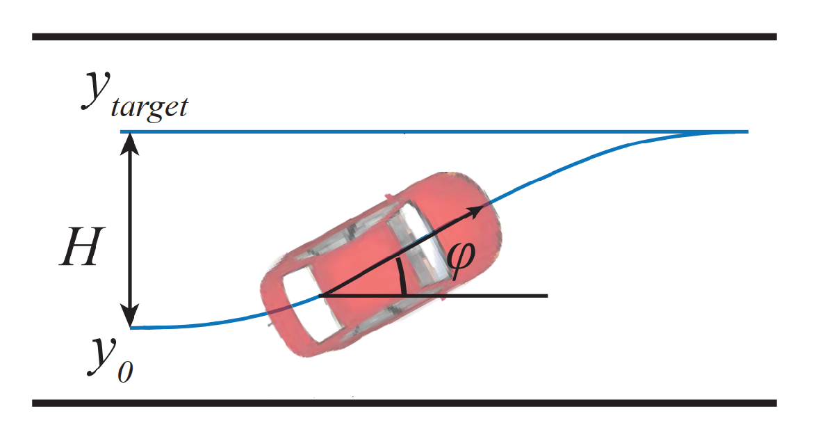
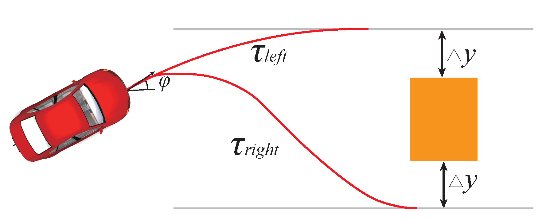
where $a_{lat}$ is the lateral acceleration in the $Fren\acute{e}t$-$Frame$, H is the total lateral distance to complete lane-change process in the $Fren\acute{e}t$-$Frame$, $t_{lat}$ is the total lateral motion time, $y_{start}$ is the initial lateral position before the lateral motion, and $y_{target}$ is the terminal lateral position, as shown in Figure 4. Given the maximum lateral acceleration $a_{max,lat}$ and the total lateral distance H, the total lateral motion time $t_{lat}$ moving from $y_0$ to $y_{target}$ can be obtained.

$$t_{lat}=\sqrt{2\pi H/a_{max,lat}}$$

(2)

The vehicle is assumed to move longitudinally with a constant acceleration.

$$v_{lon}\left(t\right)=v\left(0\right)+at$$

(3)

Thus, the heading angle during the process of lateral motion can be obtained.

$$tan\phi \left(t\right)=v_{lat}\left(t\right)/v_{lon}\left(t\right)$$

(4)

In order to generate the virtual lateral trajectories representing the corresponding behavioral semantics, it is necessary to find the appropriate target lateral position. In structured roads, the target lateral position can be selected based on the positions of obstacles and the centerline of the target lane. On an unstructured road, the appropriate target lateral position can be selected based on the positions of obstacles and the reference path provided by the global path planner. The minimum distance between the target lateral position and the boundary of obstacles is $△y$. According to the relationship between the heading angle of the vehicle in the $Fren\acute{e}t$-$Frame$ and the target lateral position, there are two cases, the details are as follows.

(1) If the heading angle in the $Fren\acute{e}t$-$Frame$ is consistent with the direction of the target lateral position, as shown in Figure 3b, the long-term virtual trajectory for the left-side evasive maneuver can be obtained by utilizing the evasive motion model. Assuming that the vehicle follows the evasive motion model in Equation (1) and the current heading angle is $\phi$, the time $t_{\phi }$ required since the vehicle initiates lateral motion can be derived. If a lateral terminal position $y_{target}$ and current lateral terminal position $y_{current}$ in the $Fren\acute{e}t$-$Frame$ are determined, $y_0$ and $t_{\phi }$ can be obtained by sampling the $y_0$ and comparing $y\left(t_{\phi }\right)$ with $y_{current}$.

$$t_{\phi }=\frac{t_{lat}}{2\pi }·\arg cos\left(-\frac{t_{lat}}{H}\left(vtan\phi -\frac{H}{t_{lat}}\right)\right)$$

(5)

The total lateral motion time $t_{lat,left}$ is obtained after $y_0$ is determined. Assuming that the evasive motion during $[t_{\phi },t_{lat,left}]$ follows the evasive motion model, the remaining trajectory from the current state to the target lateral position can be obtained as shown in Figure 3b. The remaining time $t_{arrive,left}$ to arrive at the target lateral position is defined as follows.

$$t_{arrive,left}=t_{lat,left}-t_{\phi }$$

(6)

(2) If the heading angle in the $Fren\acute{e}t$-$Frame$ is inconsistent with the direction of the target lateral position, the long-term virtual trajectory for the right-side evasive maneuver can be obtained as shown in Figure 3c. The virtual trajectory is divided into two parts. In the first part, the vehicle adjusts its heading angle to be parallel to the reference line. The lateral motion time for the first part is $t_{adj}$. The vehicle is assumed to move at constant lateral acceleration $a_{lat,adj}$ during $[0,t_{adj}]$. In the second part, the trajectory obeys the evasive motion model. The lateral motion time for the second part is $t_{lat,right}$. The remaining time $t_{arrive,right}$ to arrive at the right-side target lateral position is as follows.

$$\begin{array}{c}\hfill t_{adj}=v_{lat}/a_{lat,adj}\end{array}$$

(7a)

$$\begin{array}{c}\hfill t_{arrive,right}=t_{lat,right}+t_{adj}\end{array}$$

(7b)

2.2. Short-Term Motion Trajectory Prediction Based on Motion Model

Schubert R. et al. [27,28] compared different motion models and reached the conclusion that the CTRA model provides better performance than the constant turn rate and velocity (CTRV), the constant velocity (CV) and the constant acceleration (CA) models for short-term trajectory prediction. Utilizing the CTRA model, the velocity $v_x\left(t\right)$ and $v_y\left(t\right)$ can be derived based on the velocity and yaw angle [29].

$$\begin{array}{cc}v\left(t\right)=& a_{0}t+v_0\end{array}$$

(8a)

$$\begin{array}{cc}{v}_x\left(t\right)=& v\left(t\right)cos\left({\omega }_{0}t+{\phi }_0\right)\end{array}$$

(8b)

$$\begin{array}{cc}{v}_y\left(t\right)=& v\left(t\right)sin\left({\omega }_{0}t+{\phi }_0\right)\end{array}$$

(8c)

where $v\left(t\right)$ is the velocity at time t, $a_0$ is the current acceleration, $v_0$ is the current speed, ${\omega }_0$ is the current yaw rate, and ${\phi }_0$ is the current heading angle.

$${\omega }_0={\kappa }_0{v}_0$$

${\kappa }_0$ is the current path curvature. Therefore, $x\left(t\right)$ and $y\left(t\right)$ can be obtained.

$$\begin{array}{cc}\hfill x\left(t\right) =& \frac{a_0}{w_0^2}cos\left({\omega }_{0}t+{\phi }_0\right)+\frac{v\left(t\right)}{{\omega }_0}sin\left({\omega }_{0}t+{\phi }_0\right)-\frac{v_0}{{\omega }_0}sin{\phi }_0-\frac{a_0}{{\omega }_0^2}cos{\phi }_0+x_0\hfill \end{array}$$

(9a)

$$\begin{array}{cc}\hfill y\left(t\right) =& \frac{a_0}{w_0^2}sin\left({\omega }_{0}t+{\phi }_0\right)-\frac{v\left(t\right)}{{\omega }_0}cos\left({\omega }_{0}t+{\phi }_0\right)+\frac{v_0}{{\omega }_0}cos{\phi }_0-\frac{a_0}{{\omega }_0^2}sin{\phi }_0+y_0\hfill \end{array}$$

(9b)

2.3. The Most Likely Behavioral Semantics

This paper compares the similarity of two trajectories by calculating the distance between them. This paper compares the similarity of two trajectories by calculating the distance between them. the nearest N sampling points are used to calculate the results. The similarity of the trajectories is compared by calculating the weighted average distance.

$$SPD=\frac{{\sum }_{i=1}^N{w}_i·D_i}{{\sum }_{i=1}^N{\omega }_i}$$

(10)

where $D_i$ is the distance of two points at the same prediction time, $w_i$ is the coefficients. In order to prevent the uncertainty and interference in the measurement, a larger weight $w_i$ is set for the closer pair of points. A smaller distance between trajectories means that the trajectories are more similar and the driver is more likely to choose the semantic behavior. If the distance between the short-term predicted trajectory and the virtual long-term trajectory is below a threshold, the vehicle is considered to be driving in the corresponding driving maneuver.

3. Interactive Decision Making

According to the driver’s behavioral semantics, the system needs to determine whether the vehicle is in a safe driving area. If the state is safe, and there is still a certain safety margin for the driver, there should be no intervention. Otherwise, if the safety margin is reduced to a certain degree, the machine will intervene and the system will enter the semi-autonomous driving mode. The system should respect the driver’s behavioral semantics, and generate trajectories according to the driver’s current behavioral semantics if there still exists a safety margin.

3.1. The Driving Envelope for Candidate Driving Behaviors

For the obstacle avoidance scenario as shown in Figure 5, given the minimum lateral distance to the obstacle, the algorithm judges whether there is a feasible obstacle avoidance evasive corridor by searching the lateral non-obstacle position on both sides of the obstacle. If there is a feasible lateral evasive corridor, the lateral position with a suitable distance from the obstacle is selected as the innermost lateral target position, and the lateral position with a suitable distance from the boundary of road is selected as the outermost lateral target position. After the lateral target positions on both sides are selected, different levels of safety driving envelope for obstacle avoidance behavior are generated to identify the safety level of the current situation.

In this paper, the driving envelope for each driving maneuver is generated in the $Fren\acute{e}t$-$Frame$, as is shown in Figure 5. The ${\tau }_{outside}$ is the boundary trajectory, which takes the outermost lateral safe position as the target lateral position.

Trajectory ${\tau }_1$ keeps a safe distance from the front obstacle. Taking the innermost lateral safe position as the target lateral position, ${\tau }_1$ is the trajectory that longitudinally moves at a constant speed, and laterally follows the evasive motion model. If the ${\tau }_1$ for the left and the right evasive maneuvers exist and do not collide with ${\tau }_{outside}$, then the evasive maneuvers are safe for the driver. The driver can avoid a collision from both the left-side and the right-side without braking. Warnings should not be provided in this situation.

Trajectory ${\tau }_2$ is a critical trajectory with a constant longitudinal speed that will not collide with the obstacle. Taking the innermost lateral safe position as the target lateral position, ${\tau }_2$ is the trajectory that longitudinally moves at a constant speed, and laterally follows the evasive motion model. If the trajectories ${\tau }_2$ for one side cannot be generated because the safe distance for ${\tau }_2$ is not satisfied, or the ${\tau }_{outside}$ of that side collides with ${\tau }_2$, the vehicle can perform evasive behavior from that side by steering combined with braking. Then the vehicle’s evasive behavior for that side is in the level one warning zone.

Trajectory ${\tau }_3$ is a critical trajectory with a defined maximum deceleration that will not collide with the obstacle. Taking the innermost lateral safe position as the target lateral position, ${\tau }_3$ is the trajectory that longitudinally decelerates at maximum constant deceleration $a_{lonmax}$, and laterally follows the evasive motion model. If the trajectories ${\tau }_3$ for one side cannot be generated because of the safe distance for ${\tau }_3$ not being satisfied, or the ${\tau }_{outside}$ of that side collides with ${\tau }_3$, then the vehicle’s evasive behavior for that side is not safe. Then the vehicle’s evasive behavior for that side is in the level two warning zone.

3.2. Timing for Intervention

Based on the driving envelope of candidate driving maneuvers and the understanding of behavioral semantics, the system can judge the safety level of the driver’s maneuver at the decision level. The system can provide corresponding assistance to the driver. It is important to find the proper timing for providing assistance. If the system intervenes too early, it will interfere with the normal driving experience. If the intervention is too late, the system may miss the opportunity to avoid obstacles safely. It is necessary to ensure the existence of feasible obstacle avoidance trajectories during the intervention process. At the same time, it is necessary to minimize unnecessary interference with the driver.

In this paper, we determine the timing for intervention by calculating the probability of violating the driving envelope. There is a certain degree of uncertainty in the driver’s operation. When using the CTRA model, the uncertainty can be represented by a probability model, and the possible positions of each time step can be obtained. In [30], the vehicle was assumed to move according to a predefined motion model that considers uncertainty. The intervention timing was determined by the collision probability with traffic participants. In this paper, intervention timing is determined by calculating the probability of violating the safe driving envelope. When the probability of violating the safe driving envelope reaches a threshold, the system can provide a safety warning and intervention. This proposed method can guarantee that the collision avoidance trajectories exist when the system provides assistance.

The state of the vehicle is defined as $X={[x,y,\theta ,v,a,\omega ]}^T$, where $(x,y)$ stands for the vehicle position, $\theta$ stands for the yaw angle, v stands for the vehicle velocity, a represents the acceleration, and $\omega$ represents the yaw rate. The state vector of the vehicle at $k+1(k=0,1,2,...)$ is $X(k+1)$. The nonlinear motion model is described in Equation (11).

$$X(k+1)=\left(\begin{array}{c}x(k+1)\\ y(k+1)\\ \theta (k+1)\\ v(k+1)\\ a\\ \omega \end{array}\right)=X\left(k\right)+\left(\begin{array}{c}\Delta x\left(k\right)\\ \Delta y\left(k\right)\\ \omega T\\ aT\\ 0\\ 0\end{array}\right)+W\left(k\right)$$

(11)

where T is the sampling period. The process noise vector $W\left(k\right)$ corresponds to a zero-mean white Gaussian noise, representing noises in acceleration and yaw rate. The relationship between the noise vector and the covariance matrix is $E\left[W{W}^T\right]=Q$. The covariance matrix $Q=diag(0;0;0;0;{\sigma }_a^2;{\sigma }_{\omega }^2)$. $\Delta x\left(k\right)$ and $\Delta y\left(k\right)$ are defined as follows.

$$\begin{array}{cc}\hfill \Delta x\left(k\right)=& \frac{1}{{\omega }^2}[(v\left(k\right)\omega +a\omega T)sin(\theta \left(k\right)+\omega T)+acos(\theta \left(k\right)+\omega T)-v\left(k\right)\omega sin\theta \left(k\right)-acos\theta \left(k\right)]\hfill \\ \hfill \Delta y\left(k\right)=& \frac{1}{{\omega }^2}[(-v\left(k\right)\omega -a\omega T)cos(\theta \left(k\right)+\omega T)+asin(\theta \left(k\right)+\omega T)+v\left(k\right)\omega cos\theta \left(k\right)-asin\theta \left(k\right)]\hfill \end{array}$$

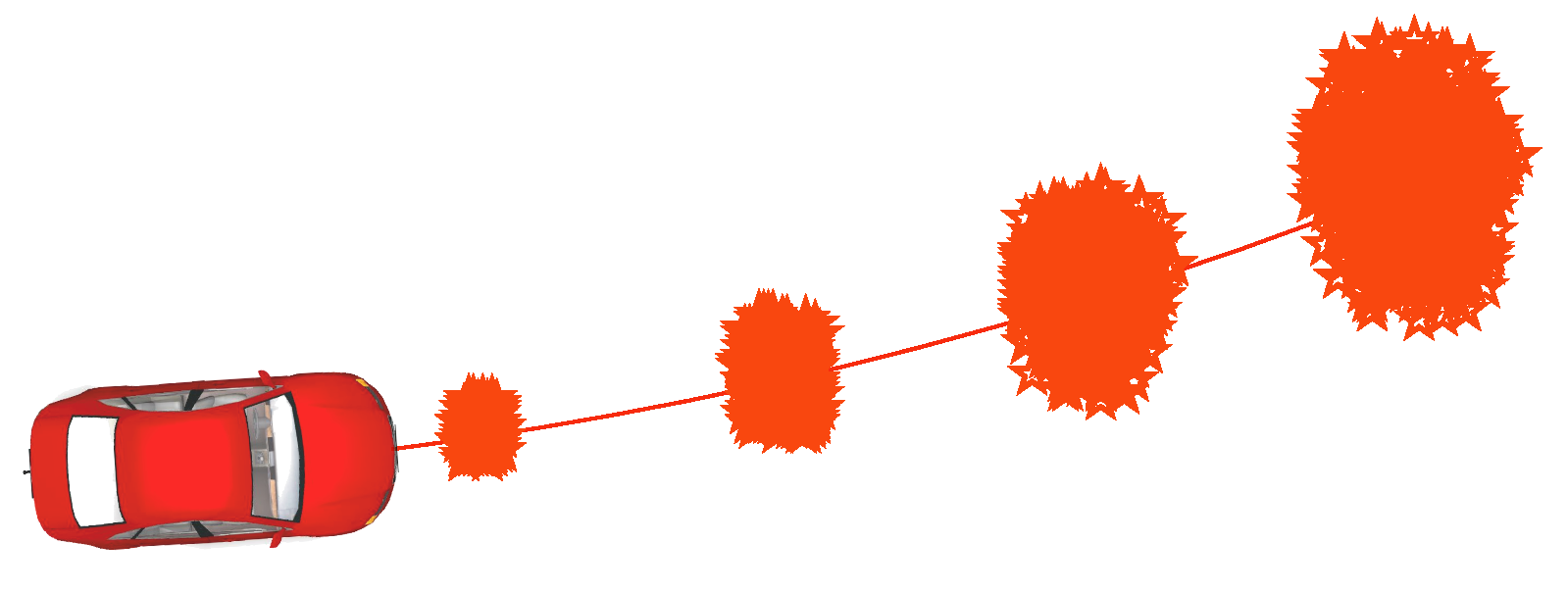
Given the vehicle state and the covariance within a predefined prediction horizon, we randomly generate N particles for each future time step. For example, the prediction results at the future time steps of 0.5 s, 1 s, 1.5 s, and 2 s are shown in Figure 6.

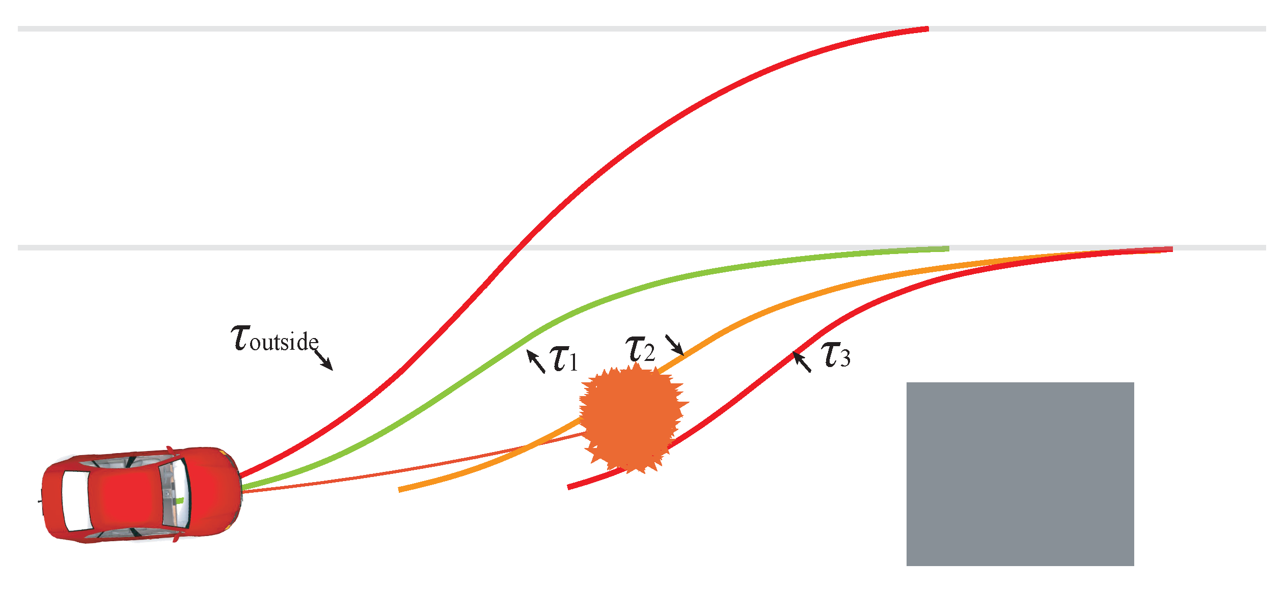
For each particle, we check if the particle is outside of the driving envelope of different safety levels, as shown in Figure 7. The more particles outside the driving envelope, the greater the probability of violating the driving envelope. The probability of violating the driving envelope is defined as follows.

$$p_{outside}=\frac{N_{outside}}{N}$$

(12)

where $N_{outside}$ denotes the number of particles outside of the driving envelope.

In order to reduce the computational cost of computing the probability of violating the driving envelope, we compute the predicted position $(x_T,y_T)$ at the predefined time T without considering the uncertainty at first. If the position $(x_T,y_T)$ is near enough to the boundary of driving envelope, then we generate the particles and compute the probability.

If the probability of violating the driving envelope of a specific safety level reaches a certain threshold, the system can provide the corresponding assistance to the driving, such as warning or intervention. For example, the generated particles at the future time step of 1.5 s are shown in Figure 7. If the $p_{outside}$ of outside the trajectory ${\tau }_2$ is beyond a threshold, the system can provide a safety warning. If the $p_{outside}$ of outside the trajectory ${\tau }_3$ is beyond a threshold, the system can provide intervention.

3.3. Evaluation of Driving Behaviors

For obstacle avoidance behavior, the safety of driving behaviors can be obtained according to the driving envelope. If the current driving behavior is unsafe, the algorithm can choose a safe driving behavior through behavioral decision-making. Besides, a cost function is designed to evaluate the quality of driving behaviors. The collision avoidance scenario is shown in Figure 8.

The designed cost function for evaluating the evasive maneuver is as follows. In this cost function, the evasive behavior of steering combined with braking is considered.

$$J={\omega }_1{t}_{arrive}^2+{\omega }_2{a}_{req,ev}^2$$

(13)

where $t_{arrive}$ is the time to arrive at the safe target lateral position next to the obstacle, which is defined in Equations (6) and (7), and $a_{req,ev}$ is the minimum required deceleration to ensure that no collision occurs.

The designed cost function for stopping to avoid collision is as follows.

$$J_{brake}={\omega }_0{a}_{req,br}^2$$

(14)

where $a_{req,br}$ is the minimum required deceleration to ensure that no collision occurs.

$$a_{req,br}=\frac{v_m^2}{2d}$$

(15)

4. Human–Machine Cooperative Trajectory Planning

There are three main objectives for human–machine cooperative trajectory planning. The first one is that the behavior of the machine should satisfy the driver’s intentions as much as possible. The second one is ensuring the least modifications to the driver’s intentions, and only intervening when necessary. Third, driving comfort and safety need to be ensured.

Most of the existing semi-autonomous driving systems use the model predictive control algorithm, which needs precise vehicle model parameters, including tire parameters, body mass, friction coefficient, etc. In [31], data-driven adaptive dynamic programming and an iterative learning scheme were adopted for learning the control law of semi-autonomous driving for lane keeping. In references [32,33], the authors put forward a Takagi–Sugeno fuzzy model-based shared control method for lane-keeping assistance systems. In reference [34], the system intervened when the vehicle deviated from the reference path by a certain distance, or the steering angle deviated from the reference steering angle to a certain degree. Given a predefined path, the output was obtained by solving the control optimization problem. In this paper, semi-autonomous driving is realized from the perspective of trajectory planning. The vehicle does not need to follow a predefined target path. The system can analyze the safety of candidate driving maneuvers using the proposed method in Section 3, and plan a safe trajectory. The trajectory is generated according to the driver’s behavioral semantics at the decision level, and according to the driver’s input at the operational level.

In [35,36], an approach that provides a flexible way to allocate authority for semi-autonomous driving is proposed. The paper focuses on the situations wherein the vehicle is always in the semi-autonomous driving mode: the driver performs the evasive maneuver to avoid collisions when the obstacles are undetected by the system. At the trajectory generation level, the machine generates trajectories using polynomials and evaluates the trajectories according to the driver’s input. Compared with the previous literature about semi-autonomous driving, this paper does not set a fixed path for the vehicle to follow, and the weight of the human–machine control authority is not fixed. Differently from the semi-autonomous driving approach proposed in [35,36], in this paper, we study the situations where the obstacles are detected by the system, and the system assists the driver to avoid collisions. The conditions for initiating the intervention are introduced in Section 3. The system enters the semi-autonomous driving mode only when the system detects a dangerous situation, so that the frequency of interventions can be reduced during normal driving situations. In addition, this paper considers more constraints than the method proposed in [35,36].

In this paper, the trajectory planning problem is decomposed into high-level behavioral decision-making problems and low-level trajectory planning problems within the safe boundaries. The trajectory algorithm in this paper generates safe motion boundaries for different behaviors and decomposes the trajectory planning problem into sub-problems of trajectory planning within the safety boundaries corresponding to different behaviors.

4.1. Generation of Candidate Trajectories

The polynomial methods can generate trajectories with curvature-bound constraints, and obtain a suboptimal solution in the discrete solution space considering the distance to obstacles and the costs of vehicle movement [37,38]. In this paper, we generate the candidate trajectories according to the driver’s behavioral semantics if they are judged safe. The fifth-order polynomial in the $Fren\acute{e}t$-$Frame$ is used to represent the lateral and longitudinal motion.

$$\begin{array}{cc}\hfill d\left(t\right)=& c_5{t}^5+c_4{t}^4+c_3{t}^3+c_2{t}^2+c_{1}t+c_0\hfill \end{array}$$

(16a)

$$\begin{array}{cc}\hfill s\left(t\right)=& a_5{t}^5+a_4{t}^4+a_3{t}^3+a_2{t}^2+a_{1}t+a_0\hfill \end{array}$$

(16b)

The coefficients of the quintic polynomial are calculated based on the initial and the terminal states, including the values of position, velocity, and acceleration. Assuming that the initial lateral state is $\left[d_0{\dot{d}}_0{\ddot{d}}_0\right]$, and the terminal lateral state is $\left[d_T{\dot{d}}_T{\ddot{d}}_T\right]$, the following matrix can be obtained.

$$\left[\begin{array}{cccccc}{t}_0^5& t_0^4& t_0^3& t_0^2& t_0^1& 1\\ t_T^5& t_T^4& t_T^3& t_T^2& t_T^1& 1\\ 5t_0^4& 4t_0^3& 3t_0^2& 2t_0^1& 1& 0\\ 5t_T^4& 4t_T^3& 3t_T^2& 2t_T^1& 1& 0\\ 20t_0^3& 12t_0^2& 6t_0^1& 2& 0& 0\\ 20t_T^3& 12t_T^2& 6t_T^1& 2& 0& 0\end{array}\right]·\left[\begin{array}{c}{c}_5\\ c_4\\ c_3\\ c_2\\ c_1\\ c_0\end{array}\right]=\left[\begin{array}{c}{d}_0\\ d_1\\ {\dot{d}}_0\\ {\dot{d}}_1\\ {\ddot{d}}_0\\ {\ddot{d}}_1\end{array}\right]$$

(17)

By substituting $t_0=0$ and the time T into the equation, the coefficients can be obtained as follows.

$$\begin{array}{cc}\hfill \left[\begin{array}{c}{c}_2\hfill \\ c_1\hfill \\ c_0\hfill \end{array}\right]& =\left[\begin{array}{c}{\ddot{d}}_0/2\\ {\dot{d}}_0\\ d_0\end{array}\right]\hfill \\ \hfill \left[\begin{array}{c}{c}_5\hfill \\ c_4\hfill \\ c_3\hfill \end{array}\right]& ={\left[\begin{array}{ccc}{T}^5& T^4& T^3\\ 5T^4& 4T^3& 3T^2\\ 20T^3& 12T^2& 6T\end{array}\right]}^{-1}\left[\begin{array}{c}{d}_T-\left(c_2{T}^2+c_{1}T+c_0\right)\\ {\dot{d}}_T-\left(2c_{2}T+c_1\right)\\ {\ddot{d}}_T-2c_2\end{array}\right]\hfill \end{array}$$

After reaching the target lateral position, the lateral velocity and lateral acceleration are both zero. The terminal state is $\left[d_{T}00\right]$. In order to ensure that the lateral movement is safe and comfortable, the lateral acceleration needs to be within a certain range. $|\ddot{d}|⩽a_{latmax}$. The lateral motion components of the trajectory can be generated by sampling the time. Similarly, the coefficients for longitudinal motion can be obtained.

In order to keep most of the trajectories within the safety boundary to reduce the time for collision checking, the evasive motion model in Section 2.1 is used to guide the selection of parameters for generating trajectories. The time $t_{arrive}$ to arrive at the target lateral position from the current lateral position can be obtained using the evasive motion model, as introduced in Equations (6) and (7). The time $t_{bound}$ for the longitudinal motion to reach the boundary of the driving envelope can be obtained, as shown in Figure 9. The approximate total time T is in the following range.

$$T\in \left[t_{arrive}-\mathcal{E},t_{bound}+t_{arrive}+\mathcal{E}\right]$$

(18)

where $\mathcal{E}$ is a constant for adjusting the total time T.

4.2. Evaluation of Candidate Trajectories

The driver’s driving intentions need to be respected for semi-autonomous driving. In this paper, the trajectories are planned on the basis of understanding the driver’s behavioral semantics to obtain the corresponding human–machine cooperative driving trajectory.A cost function is designed to evaluate the trajectory so that the path keeps a safe distance from obstacles while keeping close to the predicted vehicle trajectory under the current steering angle. After obtaining a series of candidate trajectories, the trajectory with the lowest cost is selected. Finally, a trajectory is obtained which avoids collisions with obstacles while respecting the semantics of driving behavior.

In [35,36], the machine predicted the driver’s target lateral position; the trajectories were evaluated according to the deviation between the chosen target lateral position and the predicted target lateral position. However, when the driver makes mistakes, the predicted target lateral position according to the driver’s input may not be safe. Since the penalty for avoiding obstacles is not added in the proposed method, the system will not assist the driver in avoiding collisions with detected obstacles using the proposed trajectory evaluation cost function. In this paper, we assume that the obstacles are detected. In this paper, we only generate and evaluate trajectories for the safe target lateral positions. The way of considering the driver’s input is also different. The path which is more similar to the predicted path according to the driver’s input is given a smaller penalty so that sudden changes of the steering wheel will be reduced during the intervention process, and the chosen trajectory will be closer to the driver’s intention.

4.2.1. The Cost of the Road Boundary

The motivation for the road boundary cost is to prevent vehicles from crossing the road boundary. Drivers are usually expected to drive near the centerline of the lane. The driver may deviate from the centerline of the lane in the process of driving. In order to prevent frequent interventions in a safe situation, the lateral position of the target is allowed to deviate from the centerline of the road by a certain distance. The following cost function is designed for the road boundary.

$$J_{rb}=\left\{\begin{array}{c}{c}_{rb}{\left(l_{target}-l_{center}\right)}^2|l_{target}-l_{center}| > △l_{thresh}\hfill \\ 0|l_{target}-l_{center}| ⩽ △l_{thresh}\hfill \end{array}\right.$$

(19)

where $l_{target}$ indicates the target lateral position of the trajectory and $l_{center}$ is the lateral position of the centerline. An example of the cost of the road boundary is shown in Figure 10.

4.2.2. The Cost of Longitudinal Motion Smoothness

Vehicle motion is affected by tire friction, road conditions, vehicle inertia, engine power, etc., so longitudinal acceleration and deceleration are limited. Sudden changes in acceleration can lead to tire wear and fuel waste, and cause an uncomfortable driving experience. In order to make the velocity and acceleration change smoothly, and make the longitudinal velocity of each point be close to the reference velocity, the cost of longitudinal motion was designed to be as follows.

$$J_s=\frac{1}{N}\sum _{k=1}^N\{c_{js}{\left(\stackrel{⃛}{s}\left(k\right)\right)}^2+c_{vs}{\left(\dot{s}\left(k\right)-{\dot{s}}_f\left(k\right)\right)}^2\}$$

(20)

where $\stackrel{⃛}{s}\left(t\right)$ represents the acceleration of longitudinal motion, $\dot{s}\left(t\right)$ represents the longitudinal velocity of each point, ${\dot{s}}_f\left(t\right)$ represents the reference longitudinal velocity of each point, and $c_{js}$ and $c_{vs}$ are the weighting coefficients.

4.2.3. The Cost of Lateral Motion Smoothness

Excessive lateral acceleration can cause sudden changes in steering, which can cause an uncomfortable experience. The acceleration and speed of the lateral movement of the vehicle should change smoothly. The cost of lateral motion is designed as follows.

$$J_d=\frac{1}{N}{c}_d\sum _{k=1}^N{\left(\stackrel{⃛}{d}\left(k\right)\right)}^2$$

(21)

where $\stackrel{⃛}{d}\left(t\right)$ represents lateral jerk and $c_d$ is the weighting coefficient for lateral motion smoothness.

4.2.4. The Cost of Stability

In order to prevent the vehicle from swinging, the cost of stability is added. The higher the similarity between the selected path for this frame and the previous frame, the more stable the path will be. In order to avoid an excessive difference between the selected paths in two adjacent frames, a cost is added for evaluating the similarity between the candidate paths and the path selected in the previous frame.

$$J_{prev}=-\frac{1}{I_c}{c}_{prev}\sum _{i=1}^{I_c}\left\{{\left({\alpha }_{prev}\right)}^{i-1}dist{\left(p_{k,i},{\tau }_{prev}^{}\right)}^2\right\}$$

(22)

where ${\alpha }_{prev}\in \left(0,1\right)$ is the attenuation coefficient that increases with the path length, which is used to reduce the influence of farther waypoints on the stability cost; $c_{prev}$ is the weighting coefficient. As the distance between the waypoint and the current vehicle position increases, the influence of the waypoint is smaller. $I_c$ is the number of waypoints considered, $p_{k,i}$ is the ith waypoint on the candidate trajectory ${\tau }_k$, ${\tau }_{prev}$ is the selected trajectory in the previous frame, and $dist\left(p_{k,i},{\tau }_{pre}\right)$ represents the distance from $p_{k,i}$ to ${\tau }_{prev}$.

Frequent changes in the selected target lateral position will affect the stability of the vehicle. A penalty for the selected target lateral position is designed to improve the stability. The distance between the selected target lateral position and the current lateral position should not be too large.

$$J_{target}=c_{dif}{(y_{pre,lat}-y_{target,lat})}^2+c_{targlat}{y}_{target,lat}^2$$

(23)

where $|y_{pre,lat}-y_{target,lat}|$ is the distance between the target lateral position in this frame and the previous frame; $y_{target,lat}$ is the selected lateral position in this frame; $c_{dif}$ and $c_{targlat}$ are weighting coefficients for lateral target position.

4.2.5. The Cost of Similarity to Driving Intentions

The motivation of this cost is to fuse the driver’s input in trajectory planning. If the vehicle is in semi-autonomous driving mode, the driver and the machine have control authority at the same time. In order to make the final trajectory closer to the driving intention at the operation level, a trajectory closer to the predicted trajectory based on the driver’s input will be assigned a smaller penalty. The candidate trajectories and the trajectory predicted according to the driver’s operation are shown in Figure 11. The similarity cost reflects the similarity of the candidate trajectories to the trajectory predicted according to the driver’s operation.

$$J_{intention}=-\frac{1}{I_c}{c}_{intention}\sum _{i=1}^{I_c}\left\{{\left({\alpha }_{intention}\right)}^{i-1}dist{\left(p_{k,i},{\tau }_{pred}^{}\right)}^2\right\}$$

(24)

where ${\alpha }_{intention}\in \left(0,1\right)$ is the attenuation coefficient which increases with the path length, $I_c$ is the number of waypoints considered, $p_{k,i}$ is the ith waypoint on the candidate trajectory ${\tau }_k$, ${\tau }_{pred}$ is the predicted trajectory of the vehicle based on the driver’s manipulation, and $dist\left(p_{k,i},{\tau }_{pre}\right)$ represents the distance from $p_{k,i}$ to ${\tau }_{pred}$.

4.2.6. The Cost of Non-Crossable Obstacles

The cost of obstacles can keep the vehicle away from the obstacles, which cannot be crossed, such as pedestrians and parked vehicles. Collision with such non-crossable obstacles should be avoided.

$$J_{st{a}_i}=\frac{1}{N}{c}_{st{a}_i}\sum _{k=1}^{N}exp\left(-c_{shape}{d}_{st{a}_i}^2\right)$$

(25)

where $c_{shape}$ is a coefficient that influences the shape of the potential field of a non-crossable obstacle; $d_{st{a}_i}$ is the distance from the waypoint to the static obstacle. The distance to the non-crossable obstacle can be obtained from the dist map. The three-dimensional graphical representation of the function defined in Equation (25) is illustrated in Figure 12.

4.2.7. The Total Cost

To select the optimal trajectory among the candidate trajectories, the above evaluation indicators are weighted and summed, and the cost of each candidate trajectory can be obtained as follows.

$$J_{traj,k}=J_{rb}+J_s+J_d+J_{rev}+J_{target}+J_{intention}+J_{st{a}_i}$$

(26)

The choice of coefficients is a multi-objective optimization problem. In this paper, we tune the feasible choice for the coefficients until the balance of multiple goals is reached. For example, if there is a significant jump in the target lateral position, we increase the coefficient of stability cost to obtain a more stable path. If the trajectory is too close to the obstacle, we adjust the obstacle-related coefficient $c_{st{a}_i}$ and $c_{shape}$ to keep the vehicle far away from the obstacles. At last, the trajectory ${\tau }_{k^{*}}$ with the lowest cost is selected from the candidate trajectories set for the specific behavior.

$$k^{*}=\underset{k}{argmin}\left(J_k\right)$$

(27)

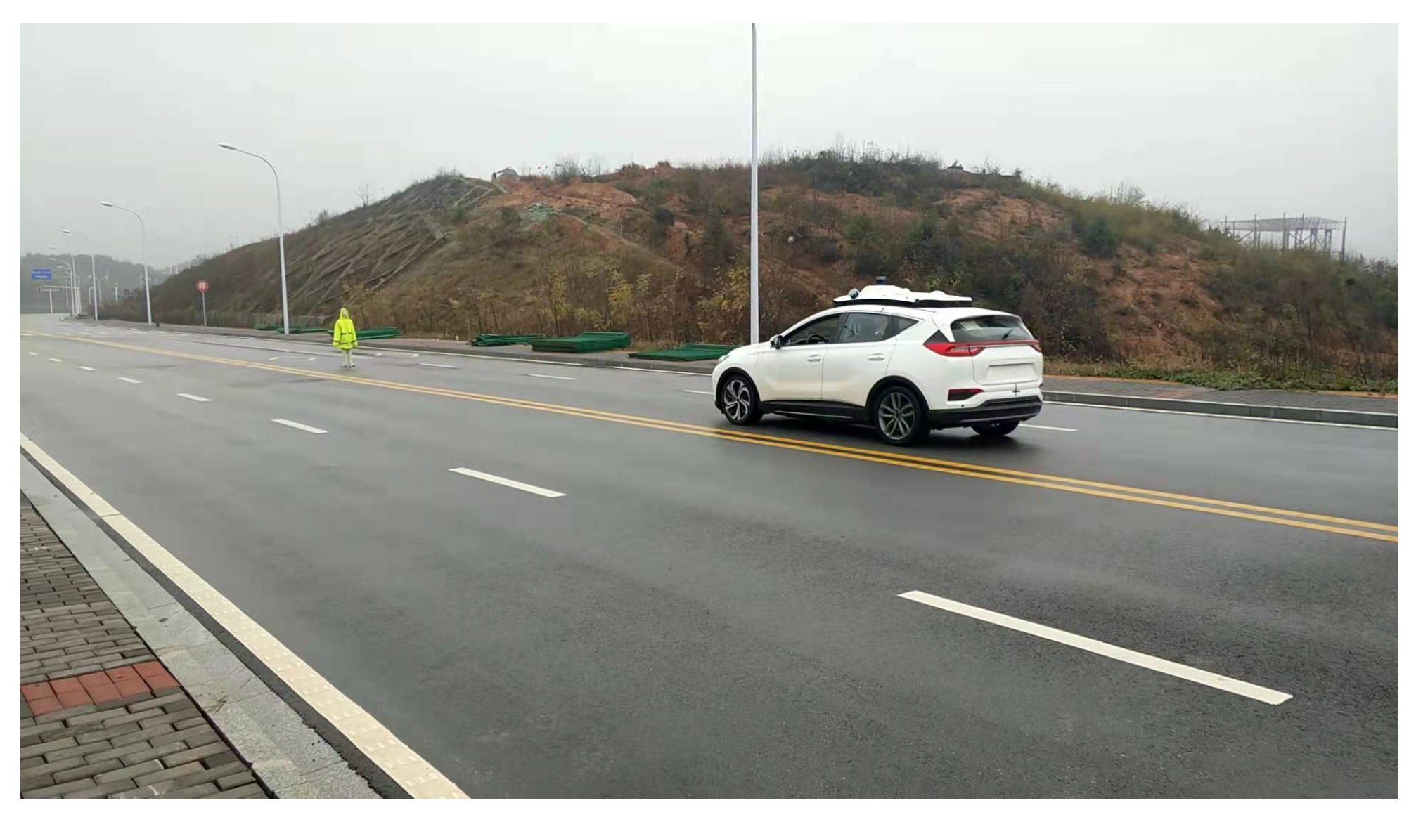
5. Experiments and Discussions

The experimental platform modified by the Red Flag EHS3 was used to test the proposed algorithm. A human drove the vehicle at about 20 km/h, and a dummy was placed in front of the vehicle. The experimental scenario is shown in Figure 13. The semi-autonomous system judged the behavioral semantics of the driver, and provided warnings and interventions when it was necessary.

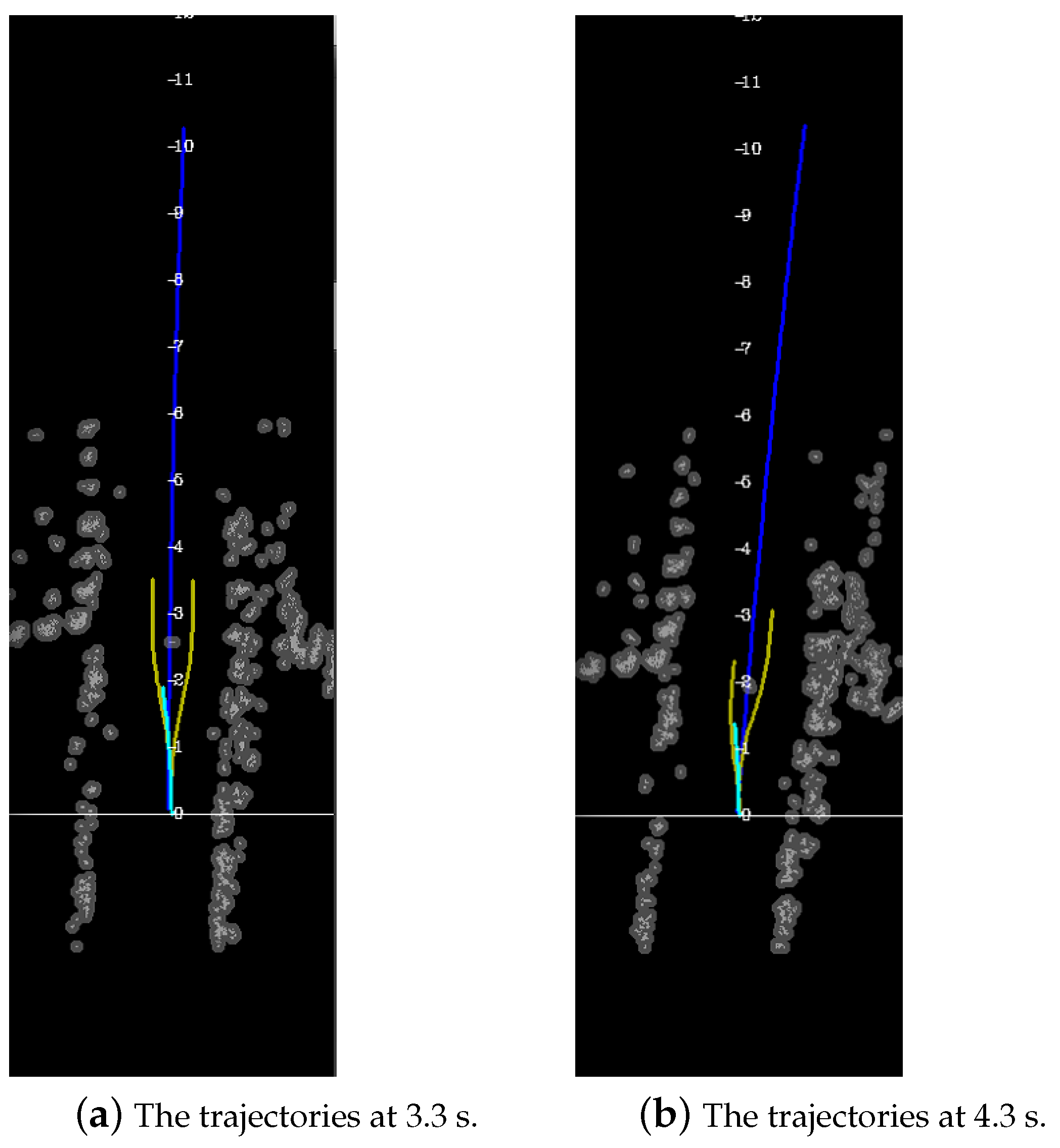
In order to resolve the conflict between the driver and the machine, the system needed to reason about the behavioral semantics of the driver. The long-term virtual trajectories of the candidate evasive maneuvers and the short-term predicted trajectory are shown in Figure 14.

The map in Figure 14 was generated based on the Lidar point cloud. As shown in Figure 14a, the dummy was about 25 m ahead. The gray parts in the pictures represent obstacles; the black part represents the non-obstacle area. A reference path is provided to clarify the direction of the road, shown as the blue line. The driver had three candidate maneuvers according to the environment, namely, a left evasive maneuver, a braking maneuver, a right evasive maneuver. The yellow lines represent the long-term virtual trajectories of evasive maneuver from the left-side and right-side of the dummy. The light green line represents the short-term predicted trajectory based on the CTRA motion model according to the current vehicle state.

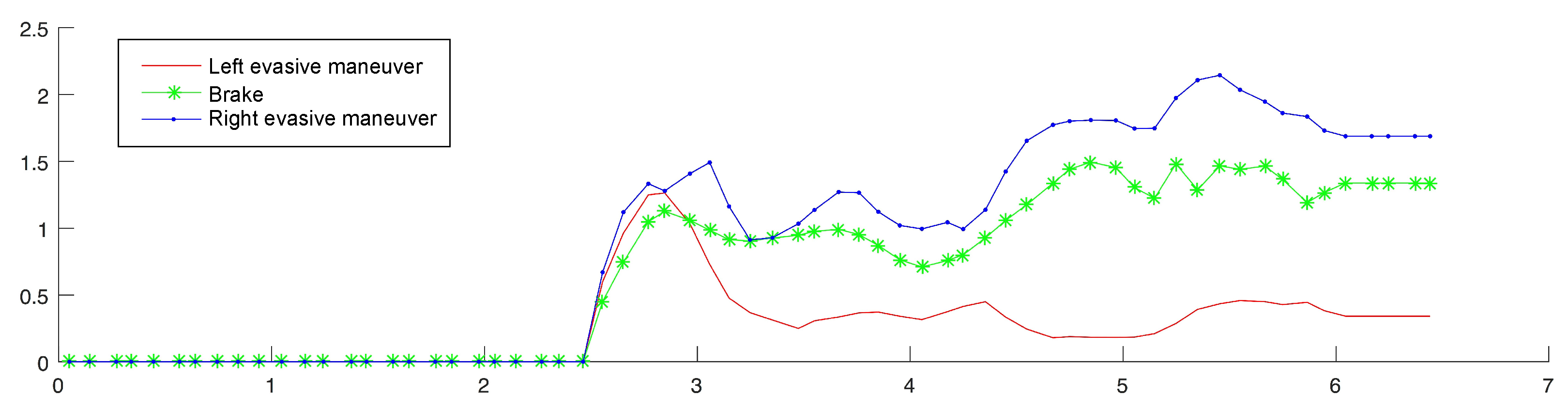
The similarities between the short-term predicted trajectory and the three candidate maneuvers can be reflected by the distances between them, which are shown in Figure 15. As is shown in Figure 15, after 3 s, the distance of the left evasive maneuver was smaller, which is in line with the actual left-side evasive maneuver.

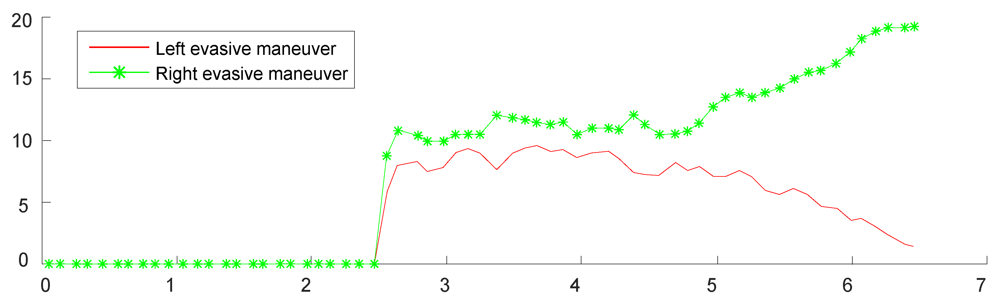
The costs for the left evasive maneuver and the right evasive maneuver are shown in Figure 16. After 5 s, the steering wheel was continuously turned to the left, the cost of avoiding obstacles on the left side gradually decreased, and the cost of avoiding obstacles on the right side gradually increased.

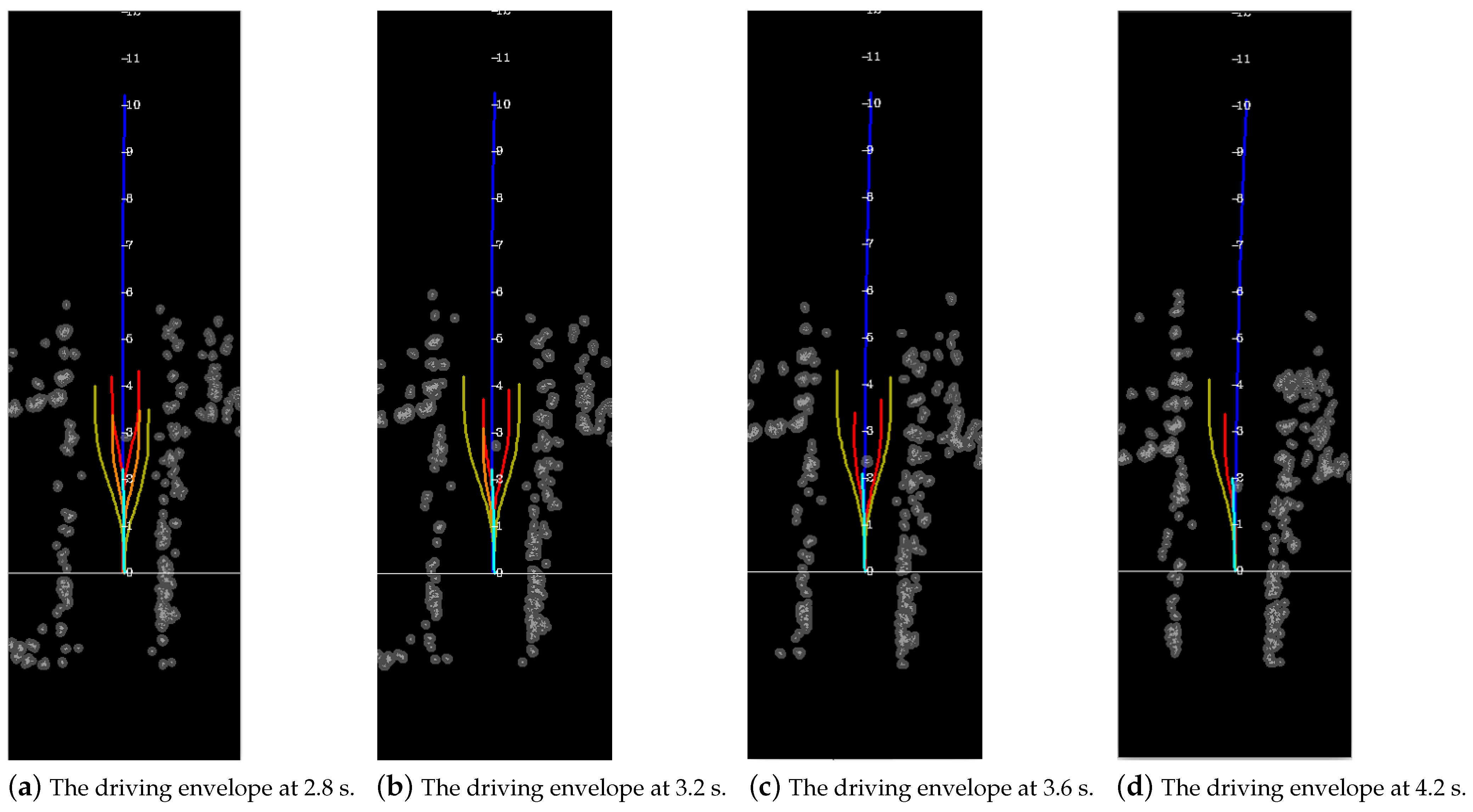
The driving envelopes of different safety levels are shown in Figure 17. The red lines represent the critical trajectory with the deceleration of −2 m/s${}^2$ that will not collide with the obstacle, corresponding to the boundary trajectory ${\tau }_3$ in Figure 5. The yellow lines represent the boundary trajectory which takes the outermost lateral safe position as the target lateral position, corresponding to the boundary trajectory ${\tau }_{outside}$ in Figure 5. The orange lines represent the critical trajectory with constant longitudinal speed that will not collide with the obstacle, corresponding to the boundary trajectory ${\tau }_2$ in Figure 5.

The system can judge the safety of evasive maneuver from the left corridor using the method proposed in Section 3. As is shown in Figure 17a, the boundary trajectory ${\tau }_2$ of safety level 2 for both sides existed; the evasive behavior for both sides could be achieved by steering. As is shown in Figure 17b, the boundary trajectory ${\tau }_2$ of safety level 2 for the right side did not exist; the boundary trajectory ${\tau }_3$ of safety level 3 for the right side existed; the right evasive behavior could be achieved by steering combined with braking, and for the left side, the collision could be avoided just by steering. At 3.2 s, as shown in Figure 15, the distance between the predicted path using CTRA model and the evasive path from the left side was smaller than that of the right side. The probability of driving from the left side was higher than that from the right side. When the probability of violating the boundary of left safety level 2 reached the predetermined threshold, the system provided a safety warning to the driver. As is shown in Figure 17c, the boundary trajectory ${\tau }_2$ of safety level 2 for both sides did not exist; the boundary trajectory ${\tau }_3$ of safety level 3 for both sides existed; the vehicle needed to slow down and steer to avoid collisions from both sides. As shown in Figure 17d, the boundary trajectory ${\tau }_3$ of safety level 3 for the right evasive behavior did not exist; it was not safe to choose the right side to avoid the collision at the deceleration of −2 m/s${}^2$. The boundary trajectory ${\tau }_3$ of safety level 3 for the left evasive behavior existed; it was safe to choose the left side to avoid the collision by braking combined with steering.

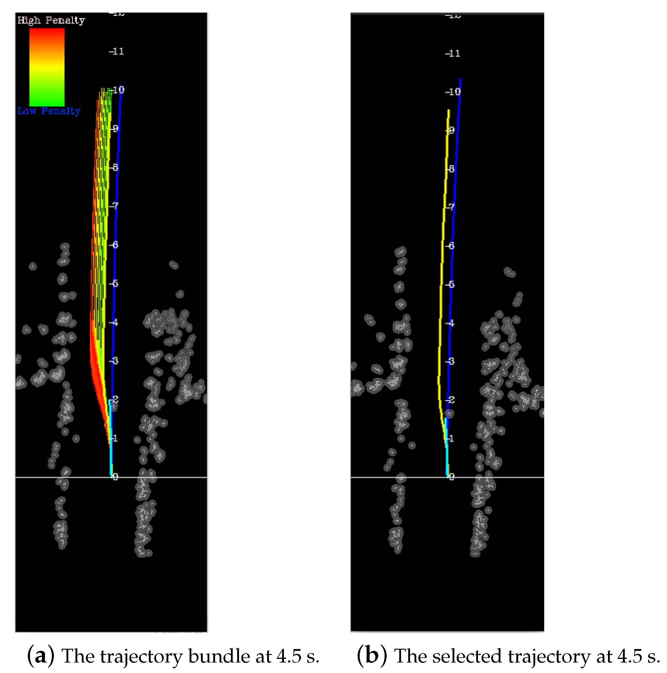
Considering the prediction results of the driver’s behavioral semantics, the system can infer that the driver is driving from the left side of the obstacle. When the probability of violating the left level 3 driving envelope reached the predefined threshold, the system started to intervene. At 4.5 s, the generated candidate trajectories from the left side of the obstacle are shown in Figure 18a. The final selected trajectory for the left side considering the input of the driver is shown in Figure 18b.

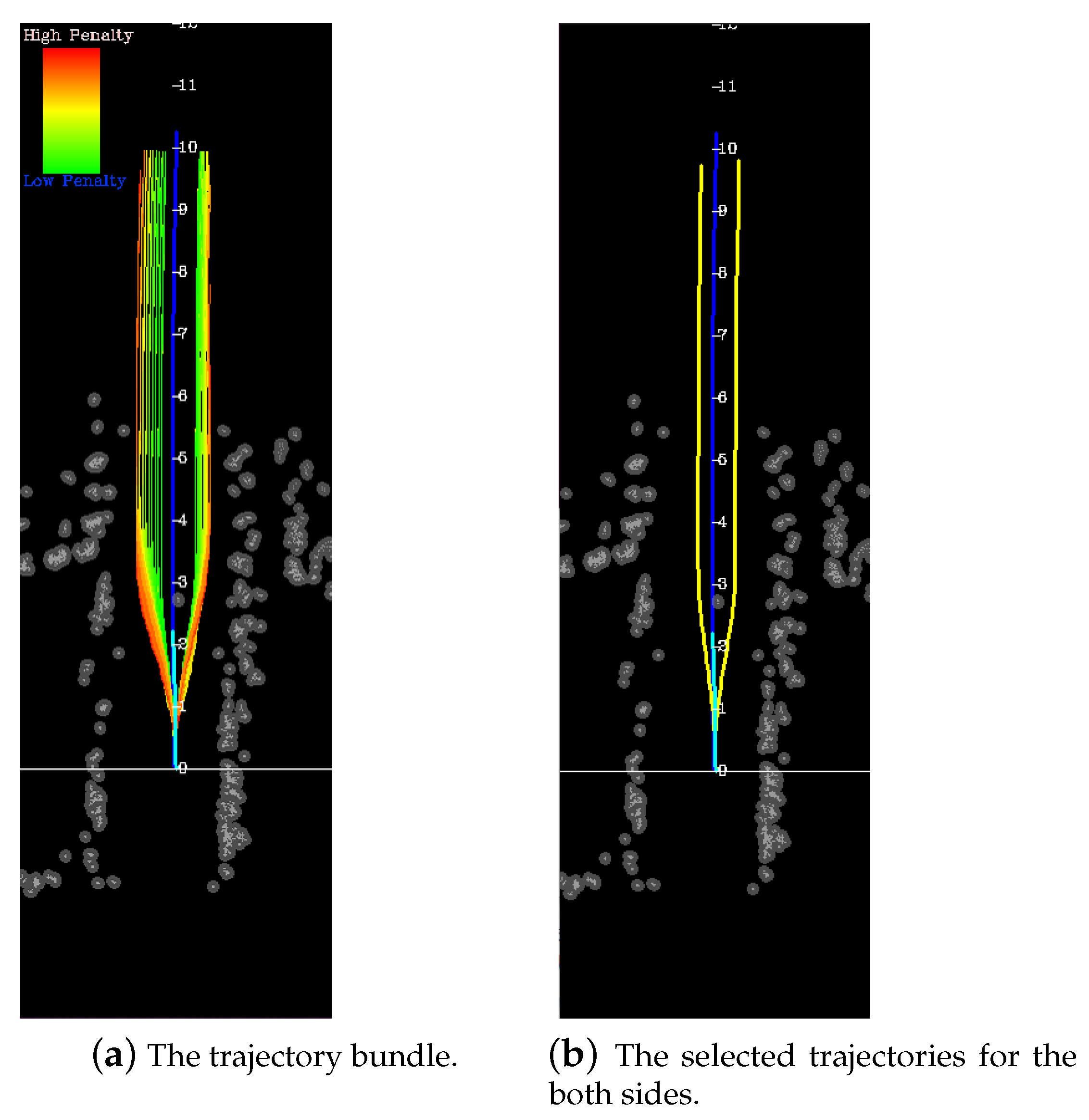
The proposed human–machine cooperative trajectory generation method can generate the trajectories according to the driver’s behavioral semantics. If the driver’s behavior semantics are not considered, and the trajectories are generated in the entire available state space, the computational burden will increase. The candidate and selected trajectories for the both candidate driving maneuvers are shown in Figure 19. Since the number of the generated trajectories was more than that of the trajectories according to the driver’s behavioral semantics, the computational time was longer. The code was implemented in C++ using an Intel I7-3520 CPU running at 3.4 GHz. The average total time for generating the trajectories for the both sides for the situation in Figure 19 was about 46 ms. The average total time for generating the trajectories for only the left side for the situation in Figure 19 was about 25 ms. The driving envelope introduced in Section 3 was used to judge the safety level of the driver’s behavioral semantics. If the state was safe, the system did not intervene. The system can generate trajectories only after a safety warning is issued and the driver does not take any corrective measures, thereby further reducing the computational burden.

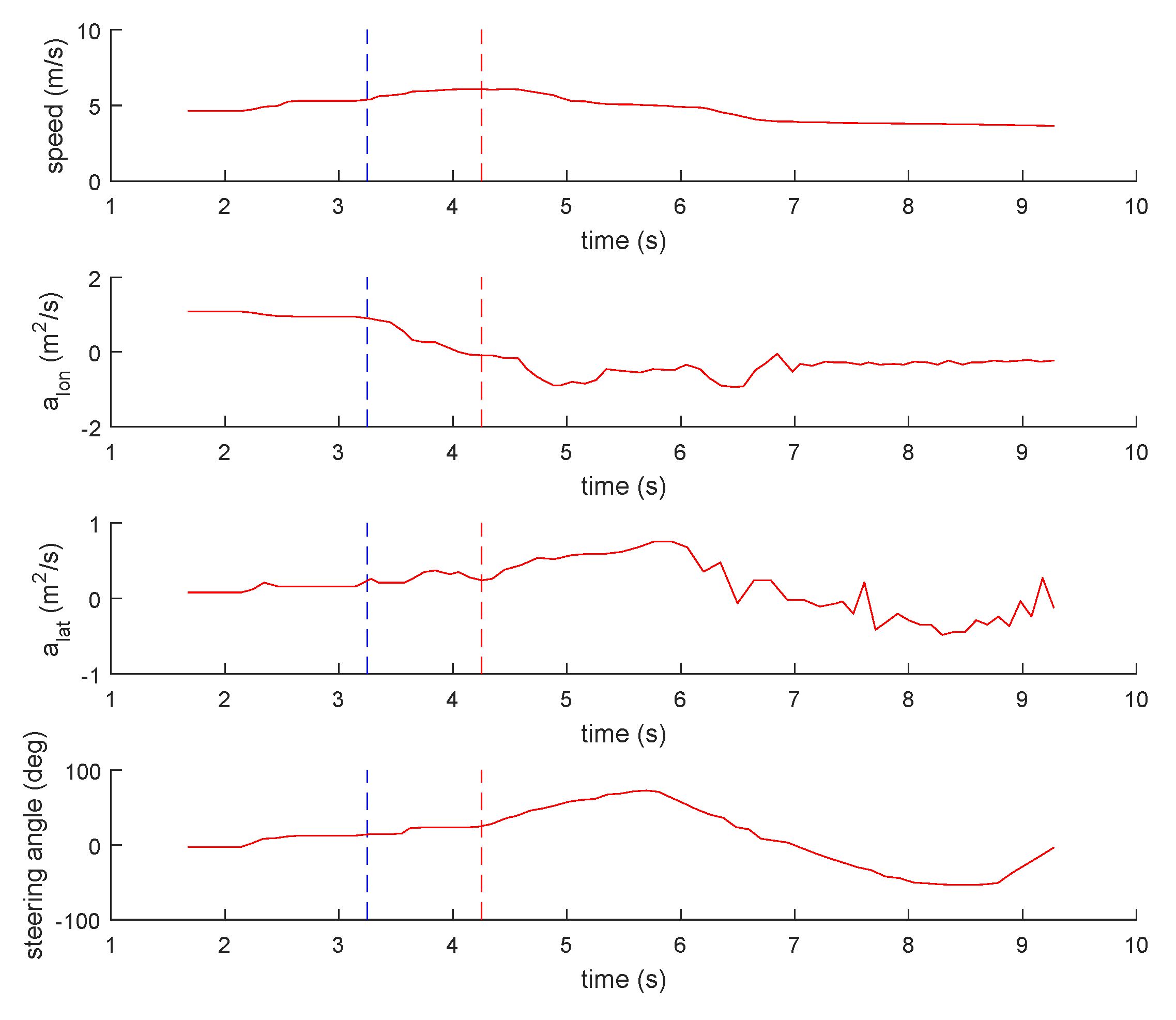
The experimental results are shown in Figure 20. The machine issued a warning at 3.2 s, when the vehicle speed was 19.5 km/h. After the warning was issued, if the driver did not take corrective action, the steering angle was insufficient for collision avoidance. The machine started a steering intervention and speed intervention at 4.3 s. The machine ended its intervention at 9.3 s, at which time the vehicle reached a safe state, and the heading angle of the vehicle was consistent with the direction of the reference path.

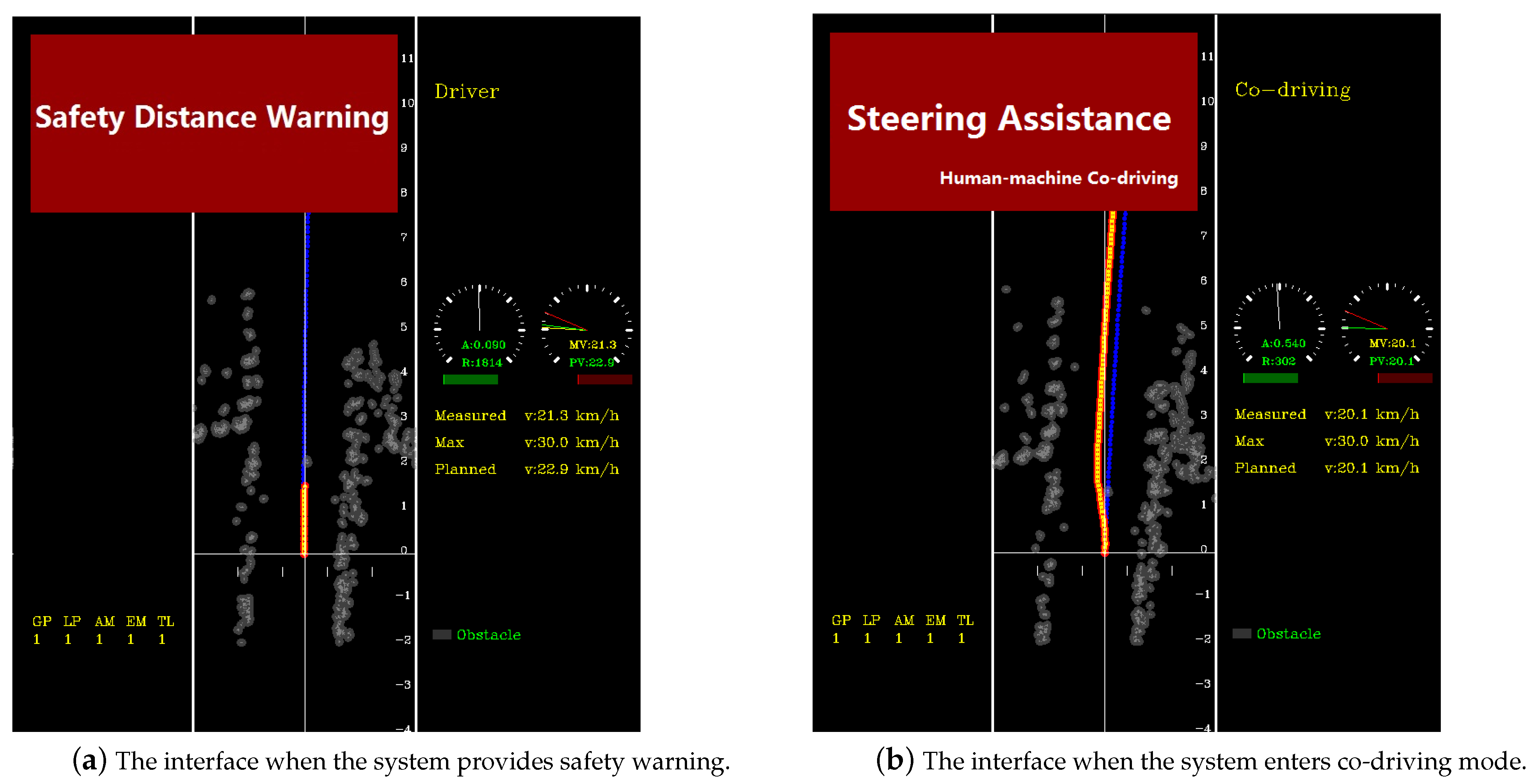
The interface of the human–machine cooperative trajectory planning program is shown in Figure 21. The interface when the system provides safety warning is shown in Figure 21a, the interface when the semi-autonomous system intervenes is shown in Figure 21b.

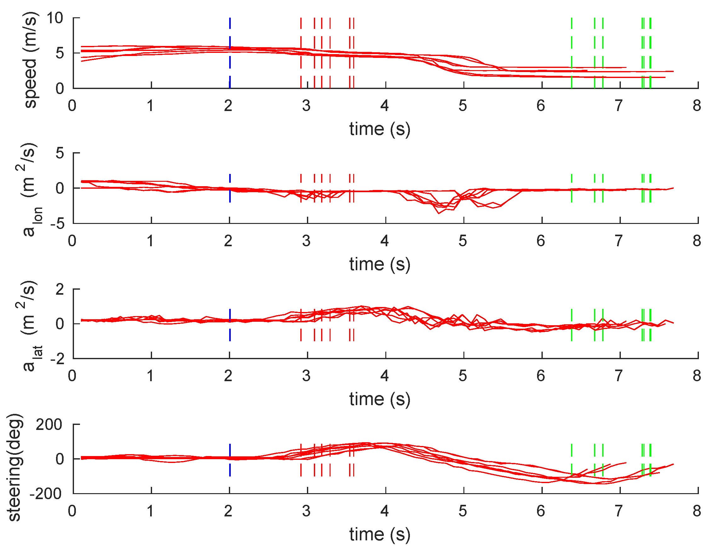
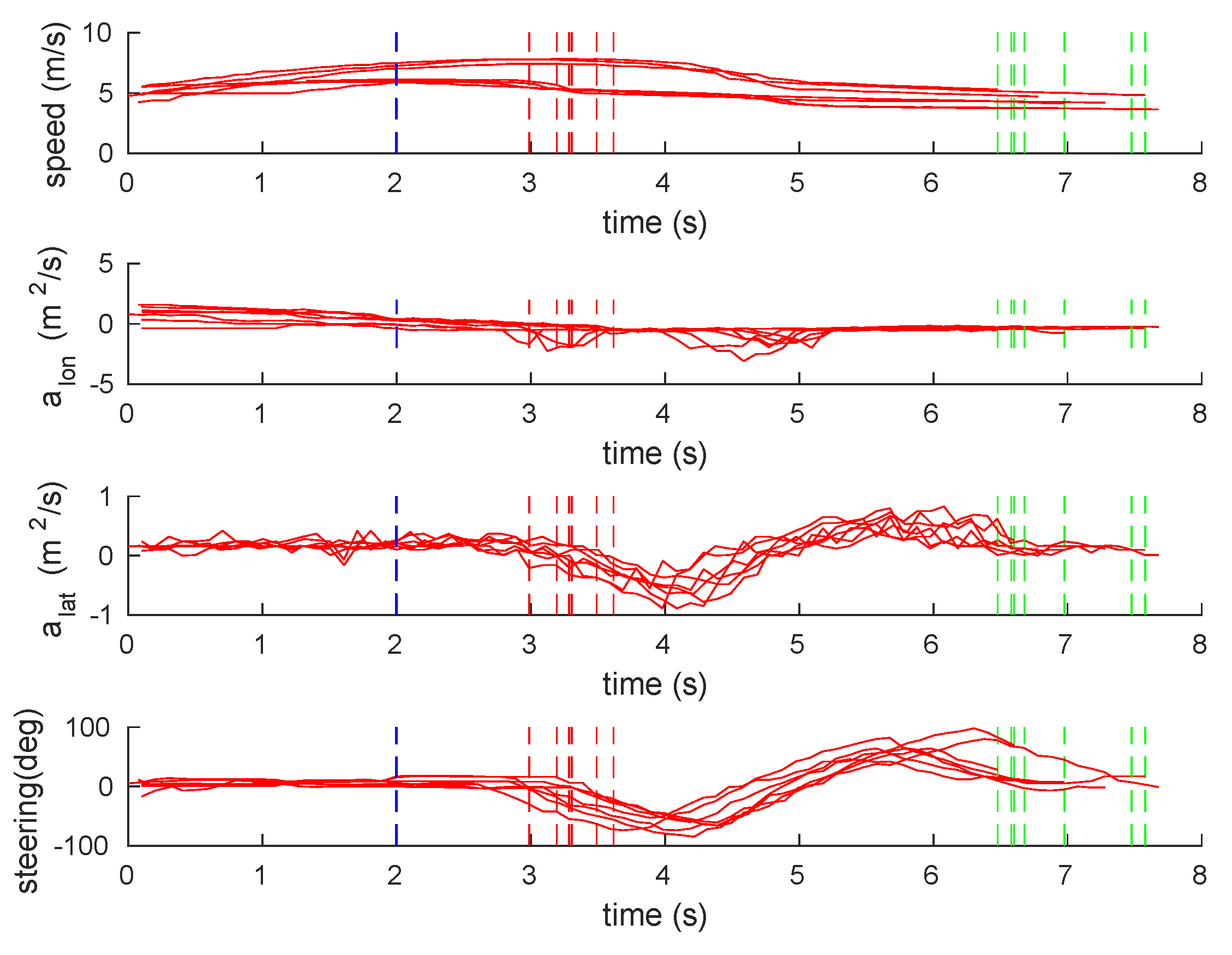
Seven drivers were invited to take the same evasive tests. The subjects were between 26 and 45 years old. The dummy was about 40 m ahead, and the vehicle’s speed was about 20 km/h. The initial lateral positions and heading angles were slightly different for each test. The experimental results of evasive action from the left side are shown in Figure 22. The experimental results of evasive action from the right side are shown in Figure 23. In order to make the picture clearer, the time axis of each set of data was shifted. The timings of providing warnings for each test were shifted to the same time.

In Figure 22 and Figure 23, the blue vertical dashed line indicates the moment when the warning was issued; the red vertical dashed line indicates the moment when the intervention was provided; the green vertical dashed line indicates the moment when the intervention was over. The experiment results show that when the vehicle is close to an obstacle and the steering angle is insufficient, the system can provide safety warnings and interventions to successfully help the driver avoid a collision with an obstacle.

The proposed method generates trajectories based on the driver’s behavioral semantics. The stability of the proposed method can be guaranteed at the decision level. Once the driver’s behavioral semantics are determined, the system can judge the safety level of the corresponding driving behavior, and generate safe trajectories for the driving behavior. If the vehicle drives straightly toward the obstacle, the system will evaluate the candidate’s driving behaviors using the method in Section 3.2 and Section 3.3. A safe driving behavior will be selected as the final decision result. The system tends to plan trajectories according to the driver’s behavioral semantics. If the driver’s behavioral semantics are not safe, the system can choose another safe driving behavior.

The proposed algorithm can provide safety warnings and interventions when the obstacle is correctly detected and the situation is judged as dangerous. The system intervenes by adding torque to the steering wheel and applying braking force to the brake pedal. If the sensor fails to detect the obstacle, the semi-autonomous driving system will not provide assistance to the driver. If the sensors detect false obstacles, and initiate interventions, the driver can exit the semi-autonomous driving mode. In the test vehicle, the driver could exit the semi-autonomous driving mode by pressing a button. If the driver’s toque on the steering wheel reaches a predefined threshold, the system can also exit the semi-autonomous driving mode.

Since the driver is in the loop, the driver may change the input during the human–machine interaction period. When the system detects that the driver’s toque is greater than zero, then the trajectory should be regenerated for each time period. Otherwise, if the driver’s torque is zero, the system will check whether the previously generated trajectory is safe. If the previous trajectory is safe, the vehicle can follow the previous planned trajectory.

6. Conclusions

In this paper, a novel human–machine cooperative trajectory planning algorithm for semi-autonomous driving was proposed. The proposed algorithm comprehensively considers the safe motion boundary constraints, driving behavioral semantics, vehicle safety limits, comfort, etc. The trajectory planning algorithm is able to obtain a trajectory that avoids collisions with dynamic obstacles while respecting the driver’s behavioral semantics at the decision level. A designed cost function is used to select a path that is close to the predicted vehicle trajectory according to the control input of the driver at the operation level. The feasibility of the proposed algorithm was validated by real vehicle experiments. The experimental results show that the proposed semi-autonomous system can issue safety warnings to the driver, and provide steering and speed interventions to successfully help the driver avoid collisions.

In this paper, the safety-related parameters in the experiments were set to be the same for different drivers. Each driver’s driving ability and driving habits were different. The maximum lateral acceleration, maximum deceleration, and reaction time vary for each driver, which will influence the timing for providing safety warnings and trajectory planning. In the future, we will continue to study the methods to extract the personal features to improve the performance of the system.