
An Interpretable Deep Learning Model for Automatic Sound Classification


Abstract
:1. Introduction
Contributions and Description of This Work
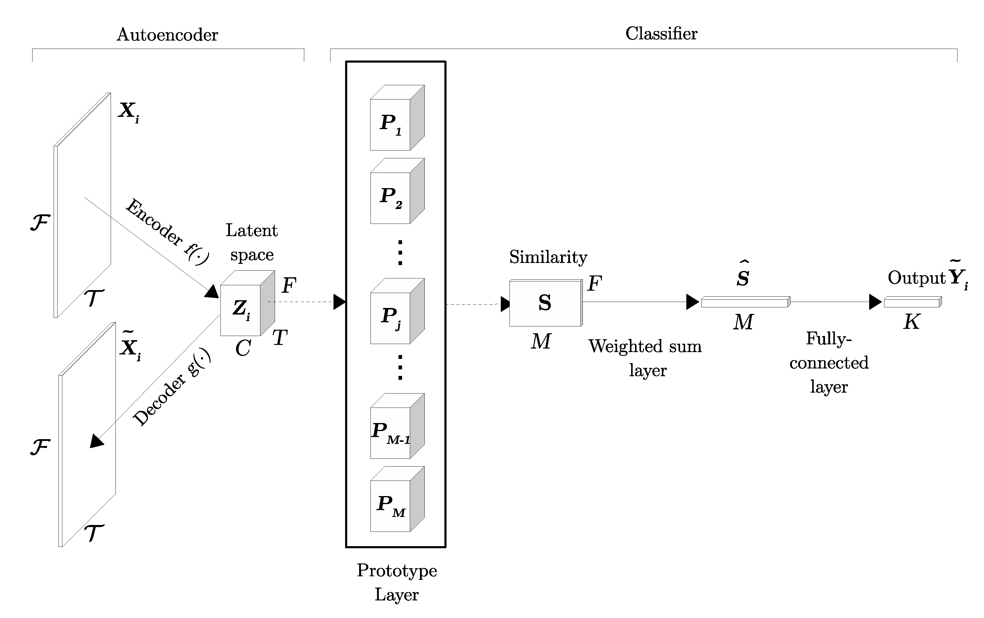
- We propose a novel interpretable deep neural network for automatic sound classification—based on an existing image classification model [21]—that provides explanations of its decisions in the form of a similarity measure between the input and a set of learned prototypes in a latent space.
- We exploit audio domain knowledge to improve the discrimination of the sound classes by designing a frequency-dependent similarity measure and by considering different time-frequency resolutions in the feature space.
- We rigorously evaluate the proposed model in the context of three different application scenarios involving speech, music, and environmental audio, showing that it achieves comparable results to those of state-of-the-art opaque algorithms.
- We show that interpretable architectures, such as the one proposed, allow for the inspection, debugging, and refinement of the model. To do that, we present two methods for reducing the number of parameters at no loss in performance, and suggest a human-in-the-loop strategy for model debugging.
2. Relation with Previous Work
3. Proposed Model
3.1. Input Representation
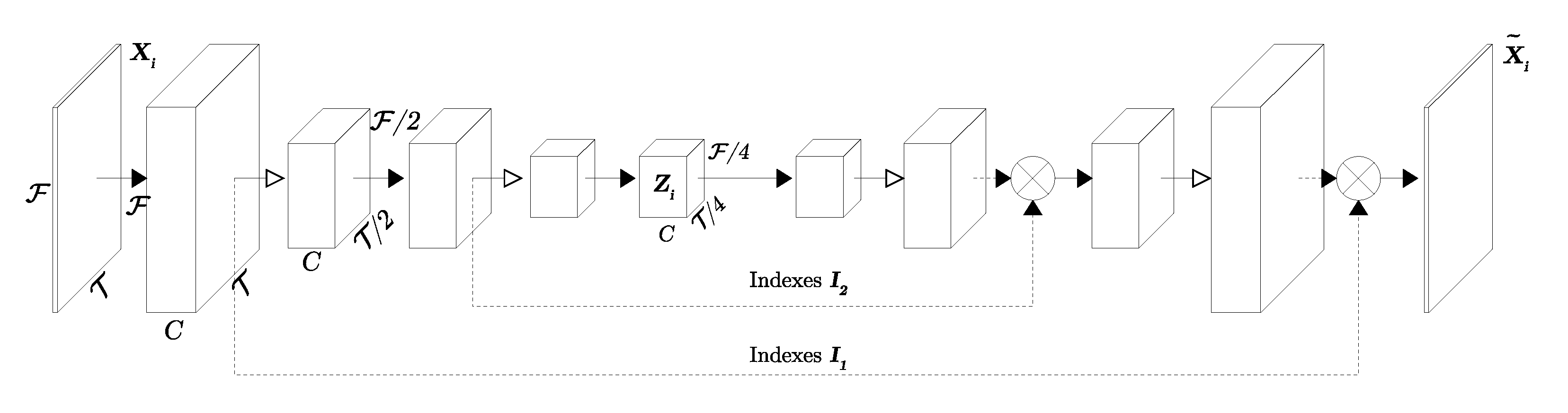
3.2. Autoencoder
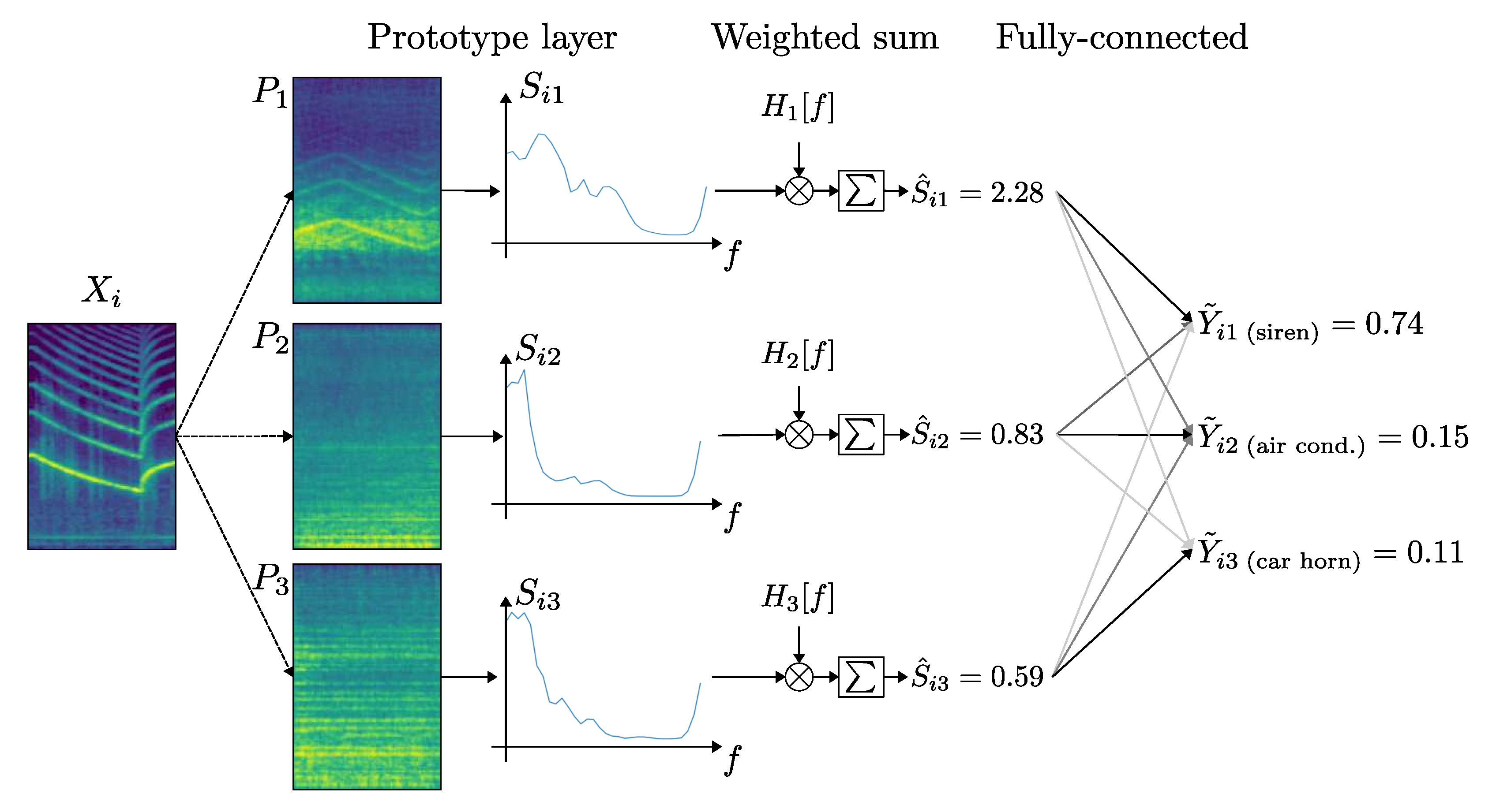
3.3. Prototype Layer
3.4. Similarity Measure and Weighted Sum Layer
3.5. Fully-Connected Layer
4. Materials and Methods
4.1. Sound Classification Tasks
4.2. Datasets
4.2.1. UrbanSound8k
4.2.2. Medley-Solos-DB
4.2.3. Google Speech Commands
4.3. Baselines
4.4. Training
5. Experiments and Results
5.1. Network Inspection
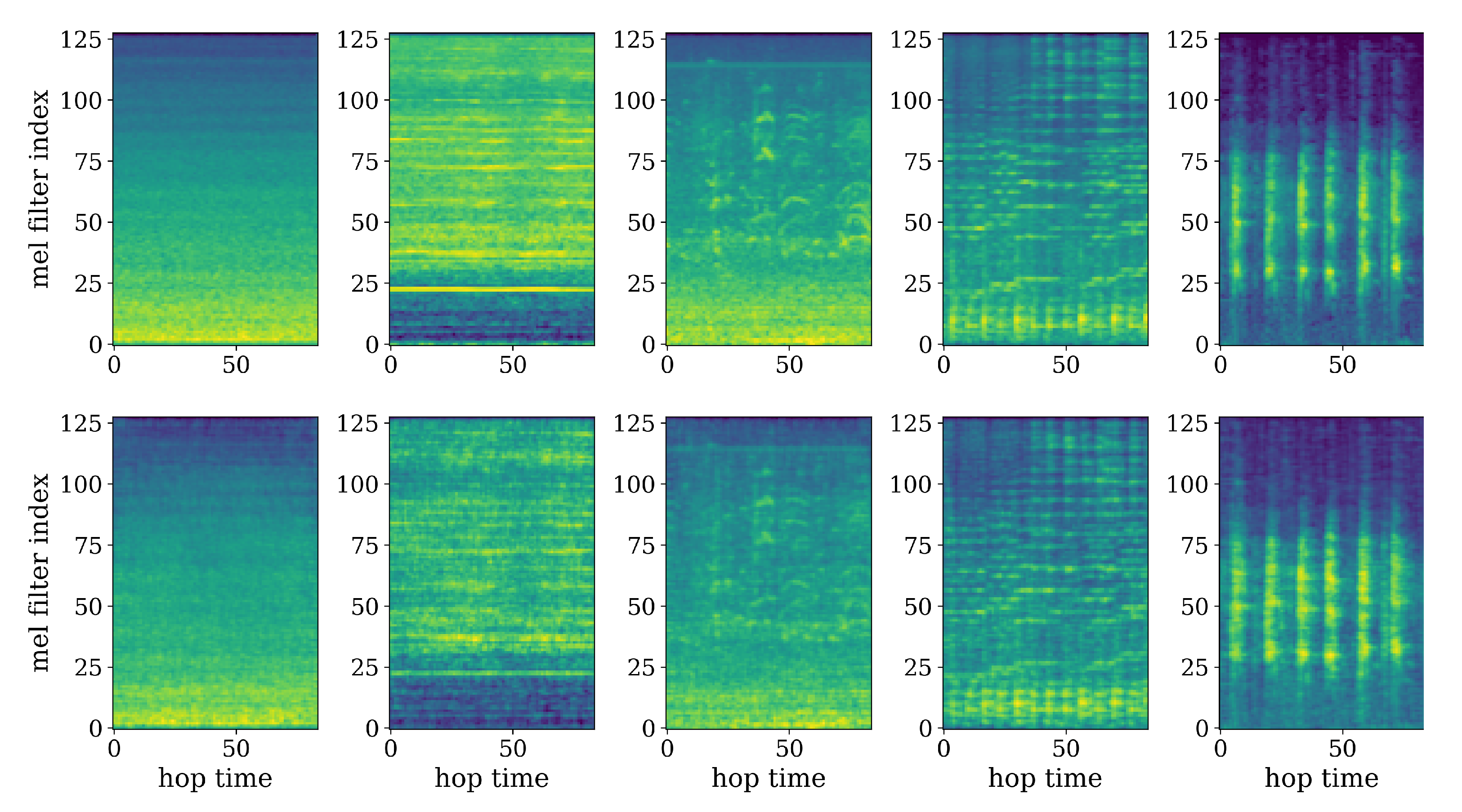
5.1.1. Autoencoder
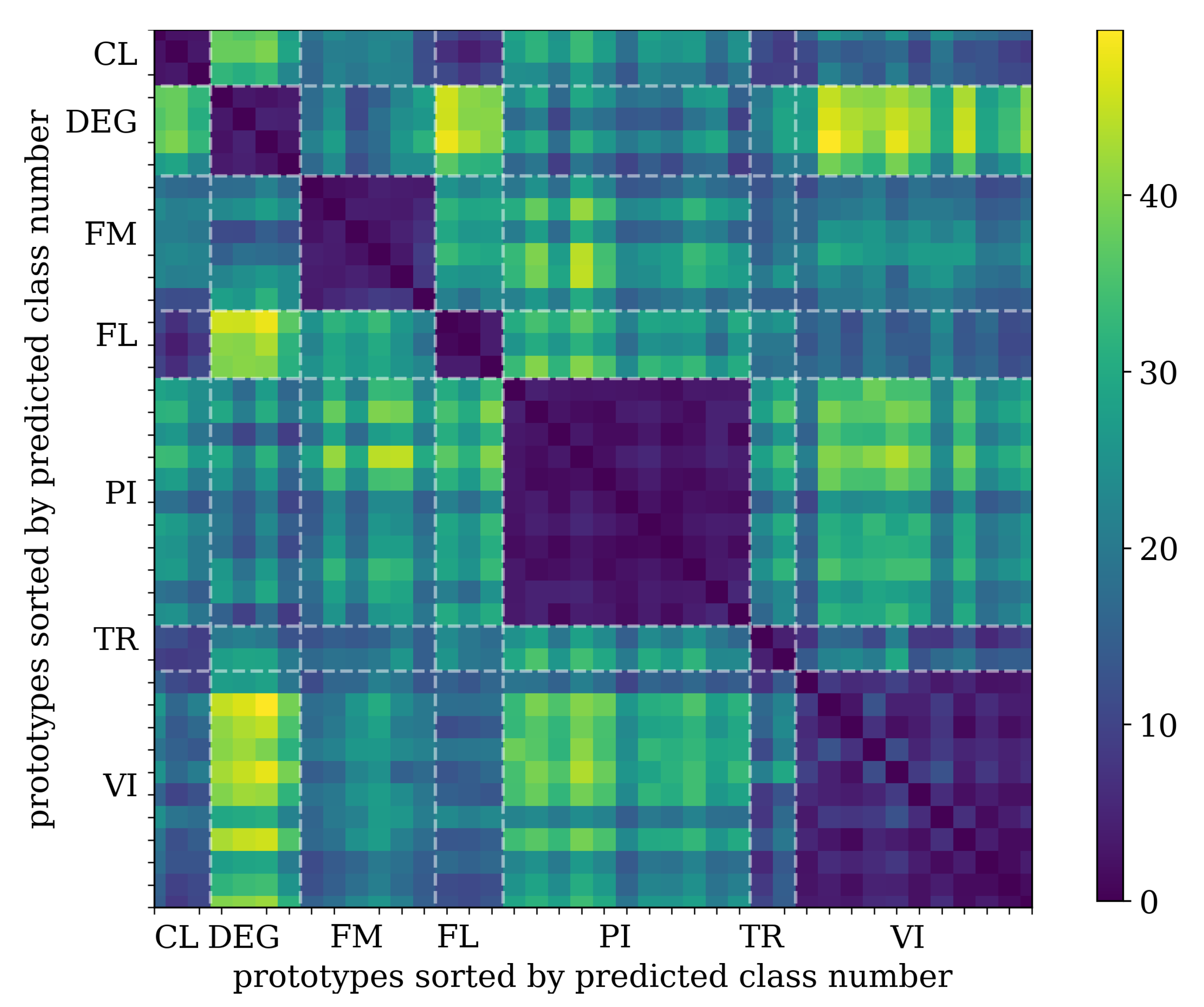
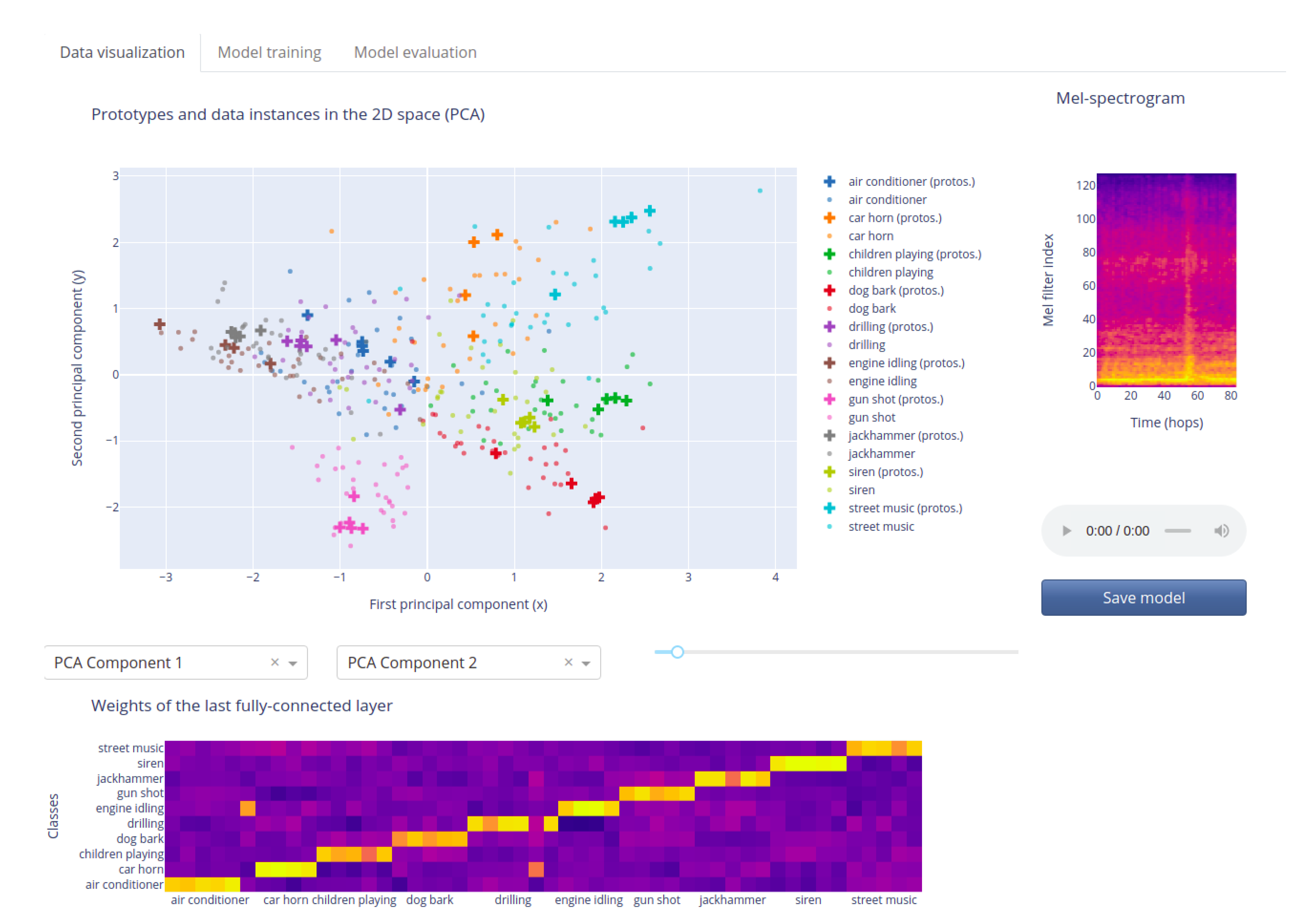
5.1.2. Prototypes
5.1.3. Fully-Connected Layer
5.1.4. Weighted Sum Layer
5.2. Network Refinement
5.2.1. Prototype Redundancy
5.2.2. Channel Redundancy
5.2.3. Manual Editing
6. Conclusions
Author Contributions
Funding
Data Availability Statement
Conflicts of Interest
Abbreviations
| AI | artificial intelligence |
| APNet | audio prototype network |
| ASC | automatic sound classification |
| CNN | convolutional neural network |
| CRNN | convolutional recurrent neural network |
| DNN | deep neural network |
| GDPR | general data protection regulation |
| GMM | Gaussian mixture model |
| LIME | local interpretable model-agnostic explanations |
| LSTM | long short-time memory |
| MFCC | mel frequency cepstral coefficients |
| MLP | multi-layer perceptron |
References
- LeCun, Y.; Bengio, Y.; Hinton, G. Deep learning. Nature 2015, 521, 56–67. [Google Scholar] [CrossRef]
- Goodfellow, I.; Bengio, Y.; Courville, A. Deep Learning; MIT Press: Cambridge, MA, USA, 2016; Available online: http://www.deeplearningbook.org (accessed on 1 January 2021).
- Krizhevsky, A.; Sutskever, I.; Hinton, G.E. ImageNet Classification with Deep Convolutional Neural Networks. In Advances in Neural Information Processing Systems 25; Pereira, F., Burges, C.J.C., Bottou, L., Weinberger, K.Q., Eds.; Curran Associates, Inc.: Red Hook, NY, USA, 2012; pp. 1097–1105. [Google Scholar]
- Peters, M.; Neumann, M.; Iyyer, M.; Gardner, M.; Clark, C.; Lee, K.; Zettlemoyer, L. Deep Contextualized Word Representations. In Volume 1 (Long Papers), Proceedings of the 2018 Conference of the North American Chapter of the Association for Computational Linguistics: Human Language Technologies, New Orleans, LA, USA, 2–7 February 2018; Association for Computational Linguistics: New Orleans, LA, USA, 2018; pp. 2227–2237. [Google Scholar] [CrossRef] [Green Version]
- Hinton, G.; Deng, L.; Yu, D.; Dahl, G.E.; Mohamed, A.; Jaitly, N.; Senior, A.; Vanhoucke, V.; Nguyen, P.; Sainath, T.N.; et al. Deep Neural Networks for Acoustic Modeling in Speech Recognition: The Shared Views of Four Research Groups. IEEE Signal Process. Mag. 2012, 29, 82–97. [Google Scholar] [CrossRef]
- Schedl, M. Deep Learning in Music Recommendation Systems. Front. Appl. Math. Stat. 2019, 5, 44. [Google Scholar] [CrossRef] [Green Version]
- Zhang, Q.; Wang, W.; Zhu, S.C. Examining CNN Representations with Respect to Dataset Bias. In Proceedings of the AAAI Conference on Artificial Intelligence, New Orleans, LA, USA, 2–7 February 2018; AAAI Press: New Orleans, LA, USA, 2018; pp. 4464–4473. [Google Scholar]
- Chen, L.; Cruz, A.; Ramsey, S.; Dickson, C.J.; Duca, J.S.; Hornak, V.; Koes, D.R.; Kurtzman, T. Hidden bias in the DUD-E dataset leads to misleading performance of deep learning in structure-based virtual screening. PLoS ONE 2019, 14, e0220113. [Google Scholar] [CrossRef]
- Menon, S.; Damian, A.; Hu, M.; Ravi, N.; Rudin, C. PULSE: Self-Supervised Photo Upsampling via Latent Space Exploration of Generative Models. In Proceedings of the IEEE/CVF Conference on Computer Vision and Pattern Recognition (CVPR), Seattle, WA, USA, 14–19 June 2020; pp. 2434–2442. [Google Scholar] [CrossRef]
- Molnar, C. Interpretable Machine Learning 2019. Available online: https://christophm.github.io/interpretable-ml-book/ (accessed on 1 January 2021).
- Rudin, C. Stop explaining black box machine learning models for high stakes decisions and use interpretable models instead. Nat. Mach. Intell. 2019, 1, 206–215. [Google Scholar] [CrossRef] [Green Version]
- Xie, N.; Ras, G.; van Gerven, M.; Doran, D. Explainable Deep Learning: A Field Guide for the Uninitiated. arXiv 2020, arXiv:2004.14545. [Google Scholar]
- Krishnan, M. Against Interpretability: A Critical Examination of the Interpretability Problem in Machine Learning. Philos. Technol. 2020, 33, 487–502. [Google Scholar] [CrossRef] [Green Version]
- Szegedy, C.; Zaremba, W.; Sutskever, I.; Bruna, J.; Erhan, D.; Goodfellow, I.; Fergus, R. Intriguing properties of neural networks. In Proceedings of the International Conference on Learning Representations (ICLR), Banff, AB, Canada, 14–16 April 2014. [Google Scholar]
- Carlini, N.; Wagner, D. Audio Adversarial Examples: Targeted Attacks on Speech-to-Text. In Proceedings of the IEEE Security and Privacy Workshops (SPW), San Francisco, CA, USA, 24 May 2018; pp. 1–7. [Google Scholar] [CrossRef] [Green Version]
- Qin, Y.; Carlini, N.; Cottrell, G.; Goodfellow, I.; Raffel, C. Imperceptible, Robust, and Targeted Adversarial Examples for Automatic Speech Recognition. In Proceedings of the 36th International Conference on Machine Learning (PMLR), Long Beach, CA, USA, 10–15 June 2019; Volume 97, pp. 5231–5240. [Google Scholar]
- Goodman, B.; Flaxman, S. European Union Regulations on Algorithmic Decision-Making and a ”Right to Explanation”. AI Mag. 2017, 38, 50–57. [Google Scholar] [CrossRef] [Green Version]
- Gilpin, L.H.; Bau, D.; Yuan, B.Z.; Bajwa, A.; Specter, M.; Kagal, L. Explaining Explanations: An Overview of Interpretability of Machine Learning. In Proceedings of the 5th IEEEInternational Conference on Data Science and Advanced Analytics (DSAA), Turin, Italy, 1–4 October 2018; pp. 80–89. [Google Scholar] [CrossRef] [Green Version]
- Zhang, Q.S.; Zhu, S.C. Visual interpretability for deep learning: A survey. Front. Inf. Technol. Electron. Eng. 2018, 19, 27–39. [Google Scholar] [CrossRef] [Green Version]
- Lipton, Z. The Mythos of Model Interpretability. Commun. ACM 2016, 61. [Google Scholar] [CrossRef]
- Li, O.; Liu, H.; Chen, C.; Rudin, C. Deep Learning for Case-Based Reasoning through Prototypes: A Neural Network that Explains Its Predictions. In Proceedings of the Thirty-Second AAAI Conference on Artificial Intelligence (AAAI-18), New Orleans, LA, USA, 2–7 February 2018; Volume 32. [Google Scholar]
- Alvarez Melis, D.; Jaakkola, T. Towards Robust Interpretability with Self-Explaining Neural Networks. In Advances in Neural Information Processing Systems; Bengio, S., Wallach, H., Larochelle, H., Grauman, K., Cesa-Bianchi, N., Garnett, R., Eds.; Curran Associates, Inc.: Red Hook, NY, USA, 2018; Volume 31, pp. 7775–7784. [Google Scholar]
- Hase, P.; Chen, C.; Li, O.; Rudin, C. Interpretable Image Recognition with Hierarchical Prototypes. In Proceedings of the The Seventh AAAI Conference on Human Computation and Crowdsourcing (HCOMP-19), Skamania Lodge, WA, USA, 28–30 October 2019; AAAI Press: Stevenson, WA, USA, 2019; Volume 7, pp. 32–40. [Google Scholar]
- Chen, C.; Li, O.; Tao, D.; Barnett, A.J.; Su, J.; Rudin, C. This Looks Like That: Deep Learning for Interpretable Image Recognition. In Advances in Neural Information Processing Systems; Wallach, H., Larochelle, H., Beygelzimer, A., d’Alché Buc, F., Fox, E., Garnett, R., Eds.; Curran Associates, Inc.: Red Hook, NY, USA, 2019; Volume 32. [Google Scholar]
- Chen, Z.; Bei, Y.; Rudin, C. Concept whitening for interpretable image recognition. Nat. Mach. Intell. 2020, 2, 772–782. [Google Scholar] [CrossRef]
- Guidotti, R.; Monreale, A.; Turini, F.; Pedreschi, D.; Giannotti, F. A Survey of Methods for Explaining Black Box Models. ACM Comput. Surv. 2018, 51. [Google Scholar] [CrossRef] [Green Version]
- Ribeiro, M.T.; Singh, S.; Guestrin, C. “Why Should I Trust You?”: Explaining the Predictions of Any Classifier. In Proceedings of the 22nd ACM SIGKDD International Conference on Knowledge Discovery and Data Mining (KDD ’16), San Francisco, CA, USA, 13–17 August 2016; Association for Computing Machinery: New York, NY, USA, 2016; pp. 1135–1144. [Google Scholar] [CrossRef]
- Yosinski, J.; Clune, J.; Bengio, Y.; Lipson, H. How transferable are features in deep neural networks. In Advances in Neural Information Processing Systems; Ghahramani, Z., Welling, M., Cortes, C., Lawrence, N., Weinberger, K.Q., Eds.; Curran Associates, Inc.: Red Hook, NY, USA, 2014; Volume 27, pp. 3320–3328. [Google Scholar]
- Kim, B.; Wattenberg, M.; Gilmer, J.; Cai, C.; Wexler, J.; Viegas, F.; Sayres, R. Interpretability Beyond Feature Attribution: Quantitative Testing with Concept Activation Vectors (TCAV). In Machine Learning Research, Proceedings of the 35th International Conference on Machine Learning, Stockholm, Sweden, 10–15 July 2018; Dy, J., Krause, A., Eds.; PMLR: Stockholmsmässan, Sweden, 2018; Volume 80, pp. 2668–2677. [Google Scholar]
- Simonyan, K.; Vedaldi, A.; Zisserman, A. Deep Inside Convolutional Networks: Visualising Image Classification Models and Saliency Maps. In Proceedings of the International Conference on Learning Representations (ICLR), Banff, AB, Canada, 14–16 April 2014. [Google Scholar]
- Adebayo, J.; Gilmer, J.; Muelly, M.; Goodfellow, I.; Hardt, M.; Kim, B. Sanity Checks for Saliency Maps. In Advances in Neural Information Processing Systems; Bengio, S., Wallach, H., Larochelle, H., Grauman, K., Cesa-Bianchi, N., Garnett, R., Eds.; Curran Associates, Inc.: Red Hook, NY, USA, 2018; Volume 31. [Google Scholar]
- Siddharth, N.; Paige, B.; Van de Meent, J.W.; Desmaison, A.; Goodman, N.D.; Kohli, P.; Wood, F.; Torr, P.H. Learning disentangled representations with semi-supervised deep generative models. arXiv 2017, arXiv:1706.00400. [Google Scholar]
- Wiegreffe, S.; Pinter, Y. Attention is not not Explanation. In Proceedings of the 2019 Conference on Empirical Methods in Natural Language Processing and the 9th International Joint Conference on Natural Language Processing (EMNLP-IJCNLP), Hong Kong, China, 3–7 November 2019; Association for Computational Linguistics: Hong Kong, China, 2019; pp. 11–20. [Google Scholar]
- Krstulović, S. Audio Event Recognition in the Smart Home. In Computational Analysis of Sound Scenes and Events; Virtanen, T., Plumbley, M.D., Ellis, D., Eds.; Springer International Publishing: Cham, Switzerland, 2018; pp. 335–371. [Google Scholar] [CrossRef]
- Bello, J.P.; Mydlarz, C.; Salamon, J. Sound Analysis in Smart Cities. In Computational Analysis of Sound Scenes and Events; Virtanen, T., Plumbley, M.D., Ellis, D., Eds.; Springer International Publishing: Cham, Switzerland, 2018; pp. 373–397. [Google Scholar] [CrossRef]
- Stowell, D. Computational Bioacoustic Scene Analysis. In Computational Analysis of Sound Scenes and Events; Virtanen, T., Plumbley, M.D., Ellis, D., Eds.; Springer International Publishing: Cham, Switzerland, 2018; pp. 303–333. [Google Scholar] [CrossRef]
- Mesaros, A.; Heittola, T.; Virtanen, T. TUT database for acoustic scene classification and sound event detection. In Proceedings of the 24rd IEEE European Signal Processing Conference 2016, Budapest, Hungary, 29 August–2 September 2016. [Google Scholar] [CrossRef]
- Kwan, C.; Ho, K.; Mei, G.; Li, Y.; Ren, Z.; Xu, R.; Zhang, Y.; Lao, D.; Stevenson, M.; Stanford, V.; et al. An Automated Acoustic System to Monitor and Classify Birds. Eurasip J. Adv. Signal Process. 2006, 2006, 1–19. [Google Scholar] [CrossRef] [Green Version]
- Salamon, J.; Bello, J.P. Unsupervised feature learning for urban sound classification. In Proceedings of the International Conference on Acoustics, Speech and Signal Processing (ICASSP), South Brisbane, QSD, Australia, 19–24 April 2015; IEEE: New York, NY, USA, 2015; pp. 171–175. [Google Scholar] [CrossRef]
- Cramer, J.; Wu, H.H.; Salamon, J.; Bello, J.P. Look, Listen and Learn More: Design Choices for Deep Audio Embeddings. In Proceedings of the 2019 IEEE International Conference on Acoustics, Speech and Signal Processing (ICASSP), Brighton, UK, 12–17 May 2019; IEEE: Brighton, UK, 2019; pp. 3852–3856. [Google Scholar]
- Salamon, J.; Bello, J.P. Deep Convolutional Neural Networks and Data Augmentation For Environmental Sound Classification. IEEE Signal Process. Lett. 2017, 24, 279–283. [Google Scholar] [CrossRef]
- Coimbra de Andrade, D.; Leo, S.; Loesener Da Silva Viana, M.; Bernkopf, C. A neural attention model for speech command recognition. arXiv 2018, arXiv:1808.08929. [Google Scholar]
- Cakir, E.; Parascandolo, G.; Heittola, T.; Huttunen, H.; Virtanen, T. Convolutional Recurrent Neural Networks for Polyphonic Sound Event Detection. Trans. Audio Speech Lang. Process. Spec. Issue Sound Scene Event Anal. 2017, 25, 1291–1303. [Google Scholar] [CrossRef] [Green Version]
- Muckenhirn, H.; Abrol, V.; Magimai-Doss, M.; Marcel, S. Understanding and Visualizing Raw Waveform-Based CNNs. In Proceedings of the Interspeech 2019, Graz, Austria, 15–19 September 2019; pp. 2345–2349. [Google Scholar] [CrossRef] [Green Version]
- Bach, S.; Binder, A.; Montavon, G.; Frederick Klauschen, K.R.M.; Samek, W. On Pixel-Wise Explanations for Non-Linear Classifier Decisions by Layer-Wise Relevance Propagation. PLoS ONE 2015, 10, e0130140. [Google Scholar] [CrossRef] [Green Version]
- Montavon, G.; Lapuschkin, S.; Binder, A.; Samek, W.; Müller, K.R. Explaining nonlinear classification decisions with deep Taylor decomposition. Pattern Recognit. 2017, 65, 211–222. [Google Scholar] [CrossRef]
- Becker, S.; Ackermann, M.; Lapuschkin, S.; Müller, K.R.; Samek, W. Interpreting and Explaining Deep Neural Networks for Classification of Audio Signals. arXiv 2018, arXiv:1807.03418. [Google Scholar]
- Schiller, D.; Huber, T.; Lingenfelser, F.; Dietz, M.; Seiderer, A.; André, E. Relevance-Based Feature Masking: Improving Neural Network Based Whale Classification through Explainable Artificial Intelligence. In Proceedings of the Interspeech 2019, Graz, Austria, 15–19 September 2019; pp. 2423–2427. [Google Scholar] [CrossRef] [Green Version]
- Mishra, S.; Sturm, B.L.; Dixon, S. Local Interpretable Model-Agnostic Explanations for Music Content Analysis. In Proceedings of the 18th International Society for Music Information Retrieval Conference ISMIR, Suzhou, China, 12–16 October 2020; pp. 537–543. [Google Scholar]
- Mishra, S.; Benetos, E.; Sturm, B.L.T.; Dixon, S. Reliable Local Explanations for Machine Listening. In Proceedings of the 2020 International Joint Conference on Neural Networks (IJCNN), Glasgow, UK, 19–24 July 2020; IEEE: Glasgow, UK, 2020; pp. 1–8. [Google Scholar] [CrossRef]
- Choi, K.; Fazekas, G.; Sandler, M.; Cho, K. Transfer learning for music classification and regression tasks. In Proceedings of the 18th International Society for Music Information Retrieval Conference ISMIR, Suzhou, China, 23–27 October 2017. [Google Scholar]
- Li, C.; Yuan, P.; Lee, H. What Does a Network Layer Hear? Analyzing Hidden Representations of End-to-End ASR through Speech Synthesis. In Proceedings of the CASSP 2020—2020 IEEE International Conference on Acoustics, Speech and Signal Processing (ICASSP), Barcelona, Spain, 4–8 May 2020; pp. 6434–6438. [Google Scholar]
- Thickstun, J.; Harchaoui, Z.; Kakade, S.M. Learning Features of Music from Scratch. In Proceedings of the International Conference on Learning Representations ICLR, Toulon, France, 24–26 April 2017. [Google Scholar]
- Lee, J.; Park, J.; Kim, K.L.; Nam, J. SampleCNN: End-to-End Deep Convolutional Neural Networks Using Very Small Filters for Music Classification. Appl. Sci. 2018, 8, 150. [Google Scholar] [CrossRef] [Green Version]
- Tax, T.M.S.; Antich, J.L.D.; Purwins, H.; Maaløe, L. Utilizing Domain Knowledge in End-to-End Audio Processing. In Proceedings of the 31st Conference on Neural Information Processing Systems (NIPS), Long Beach, CA, USA, 4–9 December 2017. [Google Scholar]
- Loweimi, E.; Bell, P.; Renals, S. On Learning Interpretable CNNs with Parametric Modulated Kernel-Based Filters. In Proceedings of the Interspeech 2019, Graz, Austria, 15–19 September 2019; pp. 3480–3484. [Google Scholar] [CrossRef] [Green Version]
- Pan, Y.; Mirheidari, B.; Tu, Z.; O’Malley, R.; Walker, T.; Venneri, A.; Reuber, M.; Blackburn, D.; Christensen, H. Acoustic Feature Extraction with Interpretable Deep Neural Network for Neurodegenerative Related Disorder Classification. Proceedings of Interspeech 2020, Shanghai, China, 25–29 October 2020; pp. 4806–4810. [Google Scholar] [CrossRef]
- Won, M.; Chun, S.; Nieto, O.; Serrc, X. Data-Driven Harmonic Filters for Audio Representation Learning. In Proceedings of the 2020 IEEE International Conference on Acoustics, Speech and Signal Processing (ICASSP), Barcelona, Spain, 4–9 May 2020; pp. 536–540. [Google Scholar] [CrossRef]
- Cakır, E.; Virtanen, T. End-to-End Polyphonic Sound Event Detection Using Convolutional Recurrent Neural Networks with Learned Time-Frequency Representation Input. In Proceedings of the 2018 IEEE International Joint Conference on Neural Networks (IJCNN), Rio de Janeiro, Brazil, 8–13 July 2018. [Google Scholar] [CrossRef] [Green Version]
- Zinemanas, P.; Cancela, P.; Rocamora, M. End-to-end Convolutional Neural Networks for Sound Event Detection in Urban Environments. In Proceedings of the 24th IEEE Conference of Open Innovations Association FRUCT, Moscow, Russia, 8–12 April 2019. [Google Scholar] [CrossRef]
- Chaki, S.; Doshi, P.; Bhattacharya, S.; Patnaik, P. Explaining perceived emotion predictions in music: An attentive approach. In Proceedings of the 21st International Society for Music Information Retrieval Conference ISMIR, Montréal, QC, Canada, 10–16 October 2020; pp. 150–156. [Google Scholar]
- Jalal, M.A.; Milner, R.; Hain, T. Empirical Interpretation of Speech Emotion Perception with Attention Based Model for Speech Emotion Recognition. Proceedings of Interspeech 2020, Shanghai, China, 25–29 October 2020; pp. 4113–4117. [Google Scholar] [CrossRef]
- Won, M.; Chun, S.; Serra, X. Toward Interpretable Music Tagging with Self-Attention. arXiv 2019, arXiv:1906.04972. [Google Scholar]
- Yang, S.; Liu, A.T.; Lee, H. Understanding Self-Attention of Self-Supervised Audio Transformers. Proceedings of Interspeech 2020, Shanghai, China, 25–29 October 2020; pp. 3785–3789. [Google Scholar] [CrossRef]
- Luo, Y.J.; Cheuk, K.W.; Nakano, T.; Goto, M.; Herremans, D. Unsupervised Disentanglement of Pitch and Timbre for Isolated Musical Instrument Sounds. In Proceedings of the 21st International Society for Music Information Retrieval Conference ISMIR, Montréal, QC, Canada, 10–16 October 2020. [Google Scholar]
- Wang, Z.; Wang, D.; Zhang, Y.; Xia, G. Learning Interpretable Representation for Controllable Polyphonic Music Generation. In Proceedings of the 21st International Society for Music Information Retrieval Conference ISMIR, Montréal, QC, Canada, 10–16 October 2020; pp. 662–669. [Google Scholar]
- Chowdhury, S.; Vall, A.; Haunschmid, V.; Widmer, G. Towards Explainable Music Emotion Recognition: The Route via Mid-level Features. In Proceedings of the 20th International Society for Music Information Retrieval Conference ISMIR, Delft, The Netherlands, 4–8 November 2019; pp. 237–243. [Google Scholar]
- De Berardinis, J.; Cangelosi, A.; Coutinho, E. The multiple voices of musical emotions: Source separation for improving music emotion recognition models and their interpretability. In Proceedings of the 21st International Society for Music Information Retrieval Conference ISMIR, Montréal, QC, Canada, 10–16 October 2020. [Google Scholar]
- Kelz, R.; Widmer, G. Towards Interpretable Polyphonic Transcription with Invertible Neural Networks. In Proceedings of the 20th International Society for Music Information Retrieval Conference ISMIR, Delft, The Netherlands, 4–8 November 2019; pp. 376–383. [Google Scholar]
- Ardizzone, L.; Kruse, J.; Rother, C.; Köthe, U. Analyzing Inverse Problems with Invertible Neural Networks. In Proceedings of the International Conference on Learning Representations, New Orleans, LA, USA, 6–9 May 2019. [Google Scholar]
- Agrawal, P.; Ganapathy, S. Interpretable Representation Learning for Speech and Audio Signals Based on Relevance Weighting. IEEE Acm Trans. Audio Speech Lang. Process. 2020, 28, 2823–2836. [Google Scholar] [CrossRef]
- Luo, J.H.; Wu, J.; Lin, W. Thinet: A filter level pruning method for deep neural network compression. In Proceedings of the IEEE International Conference on Computer Vision, Venice, Italy, 22–29 October 2017; pp. 5058–5066. [Google Scholar]
- Badrinarayanan, V.; Kendall, A.; Cipolla, R. SegNet: A Deep Convolutional Encoder-Decoder Architecture for Image Segmentation. IEEE Trans. Pattern Anal. Mach. Intell. 2017, 39, 2481–2495. [Google Scholar] [CrossRef] [PubMed]
- Maas, A.L.; Hannun, A.Y.; Ndrew Y., N. Rectifier Nonlinearities Improve Neural Network Acoustic Models. In Proceedings of the 30th International Conference on Machine Learning JMLR, Atlanta, GA, USA, 16–21 June 2013; Volume 28. [Google Scholar]
- Pons, J.; Lidy, T.; Serra, X. Experimenting with musically motivated convolutional neural networks. In Proceedings of the 2016 IEEE 14th International Workshop on Content-Based Multimedia Indexing (CBMI), Bucharest, Romania, 15–17 June 2016; pp. 1–6. [Google Scholar] [CrossRef] [Green Version]
- Salamon, J.; Jacoby, C.; Bello, J.P. A Dataset and Taxonomy for Urban Sound Research. In Proceedings of the 22nd ACM International Conference on Multimedia (MM ’14), New York, NY, USA, 3–7 November 2014; Association for Computing Machinery: New York, NY, USA, 2014; pp. 1041–1044. [Google Scholar] [CrossRef]
- Font, F.; Roma, G.; Serra, X. Freesound Technical Demo. In Proceedings of the ACM International Conference on Multimedia (MM’13), Barcelona, Spain, 21–25 October 2013; ACM: Barcelona, Spain, 2013; pp. 411–412. [Google Scholar] [CrossRef]
- Lostanlen, V.; Cella, C.E. Deep convolutional networks on the pitch spiral for musical instrument recognition. In Proceedings of the 17th International Society for Music Information Retrieval Conference ISMIR, New York, NY, USA, 7–11 August 2016. [Google Scholar]
- Bittner, R.; Salamon, J.; Tierney, M.; Mauch, M.; Cannam, C.; Bello, J. MedleyDB: A Multitrack Dataset for Annotation-Intensive MIR Research. In Proceedings of the 15th International Society for Music Information Retrieval Conference ISMIR, Taipei, Taiwan, 27–31 October 2014. [Google Scholar]
- Joder, C.; Essid, S.; Richard, G. Temporal Integration for Audio Classification With Application to Musical Instrument Classification. IEEE Trans. Audio Speech Lang. Process. 2009, 17, 174–186. [Google Scholar] [CrossRef] [Green Version]
- Warden, P. Speech Commands: A Dataset for Limited-Vocabulary Speech Recognition. arXiv 2018, arXiv:1804.03209. [Google Scholar]
- Zinemanas, P.; Hounie, I.; Cancela, P.; Font, F.; Rocamora, M.; Serra, X. DCASE-models: A Python library for computational environmental sound analysis using deep-learning models. In Proceedings of the Fifth Workshop on Detection and Classification of Acoustic Scenes and Events DCASE, Tokyo, Japan, 2–3 November 2020; pp. 240–244. [Google Scholar]
- Griffin, D.; Lim, J. Signal estimation from modified short-time Fourier transform. IEEE Trans. Acoust. Speech Signal Process. 1984, 32, 236–243. [Google Scholar] [CrossRef]
- McFee, B.; McVicar, M.; Raffel, C.; Liang, D.; Nieto, O.; Battenberg, E.; Moore, J.; Ellis, D.; Yamamoto, R.; Bittner, R.; et al. librosa: 0.4.1. Zenodo 2015. [Google Scholar] [CrossRef]


| UrbanSound8K | Medley-Solos-DB | Google Speech Commands | ||||||||||
|---|---|---|---|---|---|---|---|---|---|---|---|---|
| APNet | 22.05 | 128 | 4096, 1024 | 4.0 | 44.1 | 256 | 4096, 1024 | 3.0 | 16.0 | 80 | 1024, 256 | 1.0 |
| SB-CNN | 44.1 | 128 | 1024, 1024 | 3.0 | 44.1 | 256 | 1024, 1024 | 3.0 | 16.0 | 80 | 1024, 256 | 1.0 |
| Att-CRNN | 44.1 | 128 | 1024, 1024 | 3.0 | 44.1 | 256 | 1024, 1024 | 3.0 | 16.0 | 80 | 1024, 256 | 1.0 |
| Openl3 | 48.0 | 256 | 512, 242 | 1.0 | 48.0 | 256 | 512, 242 | 1.0 | 48.0 | 256 | 512, 242 | 1.0 |
| M | C | (, , ) | B | |
|---|---|---|---|---|
| UrbanSound8K | 50 | 32 | (10,5,5) | 256 |
| Medley-solos-DB | 40 | 48 | (10,5,5) | 96 |
| Google Speech Commands | 105 | 48 | (2,1,1) | 128 |
| UrbanSound8K | Medley-Solos-DB | Google Speech Commands | ||||
|---|---|---|---|---|---|---|
| Acc. (%) | # Params. (M) | Acc. (%) | # Params. (M) | Acc. (%) | # Params. (M) | |
| APNet | 76.2 | 1.2 | 65.8 | 4.2 | 89.0 | 1.8 |
| SB-CNN | 72.2 | 0.86 | 64.7 | 1.8 | 92.1 | 0.17 |
| Att-CRNN | 61.1 | 0.23 | 52.0 | 0.29 | 93.2 | 0.20 |
| Openl3 | 77.3 | 9.5 | 67.3 | 9.5 | 70.9 | 9.5 |
| Network | Accuracy | Approx. # Parameters |
|---|---|---|
| APNet | M | |
| APNet (R. prototypes) | M | |
| APNet (R. channels) | M | |
| Openl3 | M |
Publisher’s Note: MDPI stays neutral with regard to jurisdictional claims in published maps and institutional affiliations. |
© 2021 by the authors. Licensee MDPI, Basel, Switzerland. This article is an open access article distributed under the terms and conditions of the Creative Commons Attribution (CC BY) license (https://creativecommons.org/licenses/by/4.0/).
Share and Cite
Zinemanas, P.; Rocamora, M.; Miron, M.; Font, F.; Serra, X. An Interpretable Deep Learning Model for Automatic Sound Classification. Electronics 2021, 10, 850. https://doi.org/10.3390/electronics10070850
Zinemanas P, Rocamora M, Miron M, Font F, Serra X. An Interpretable Deep Learning Model for Automatic Sound Classification. Electronics. 2021; 10(7):850. https://doi.org/10.3390/electronics10070850
Chicago/Turabian StyleZinemanas, Pablo, Martín Rocamora, Marius Miron, Frederic Font, and Xavier Serra. 2021. "An Interpretable Deep Learning Model for Automatic Sound Classification" Electronics 10, no. 7: 850. https://doi.org/10.3390/electronics10070850