Characteristic Analysis of Fractional-Order Memristor-Based Hypogenetic Jerk System and Its DSP Implementation

Abstract

In this paper, a fractional-order memristive model with infinite coexisting attractors is investigated. The numerical solution of the system is derived based on the Adomian decomposition method (ADM), and its dynamic behaviors are analyzed by means of phase diagrams, bifurcation diagrams, Lyapunov exponent spectrum (LEs), dynamic map based on SE complexity and maximum Lyapunov exponent (MLE). Simulation results show that it has rich dynamic characteristics, including asymmetric coexisting attractors with different structures and offset boosting. Finally, the digital signal processor (DSP) implementation verifies the correctness of the solution algorithm and the physical feasibility of the system.

1. Introduction

Chaotic systems have initial sensitivity, long-term unpredictability and other excellent characteristics; therefore, they can be cross-combined with other scientific fields such as biology, information science, security, and engineering [1,2,3,4,5]. For this reason, more and more scholars are focusing on establishing new chaotic systems with better chaotic characteristics. Among them, building a memristive chaotic system is an effective method [6,7]. A memristor is a bridge connecting magnetic flux and electric charge [8], although it took a long time from the concept of the memristor to the advent of the real memristor [9]. However, in recent years, memristors have been widely studied due to their special properties, which have promoted memristors in electrical and electronics [10], communication [11], neural networks [12], biological simulation [13], and security [14] and other fields of application. In the field of chaos, memristors have become a research focus due to their rich nonlinear characteristics. For example, by introducing memristors with different properties into the existing dynamic systems, some chaotic or hyperchaotic systems with rich characteristics have been studied [15,16]. A new memristive chaotic circuit was obtained by replacing the non-linear resistor with a memristor in a chaotic circuit [17,18,19,20]. Most of these studies are based on integer-order calculus systems. Fractional-order calculus can more accurately describe physical models, so it has attracted the attention of researchers and became a focus of nonlinear research.

By combining fractional calculus and memristors, people pay more attention to the behavior of the system with its control parameters. Study results show that many fractional-order memristive systems have rich dynamic characteristics. For example, Mou et al. [21] analyzed the dynamic behavior of a 4D hyperchaotic memristive circuit with different parameters. Li et al. [22] reported a 4D system with an infinite equilibrium point of order memristor, but with further research, some scholars found that the system parameters are not the only factors that affect the dynamic characteristics of the system. Recently, Bao’s team found that some memristive systems have extreme multistability [23,24], which is reflected in the complete bifurcation path of the system with changes in initial values. For example, the memristor-based system proposed in Ref. [24] has unlimited coexistence attractors and the transition behavior is completely different from the transient chaos. Moreover, as a special dynamic characteristic, extreme multistability does not only appear in memristive systems. For example, Wan et al. [25] reported super multistability in discrete neural networks. Chen et al. [26] made a more in-depth study of extreme multistability. In Ref. [26], Chen et al. constructed a 3rd-order dimensionality-reducing flux capable of maintaining the original dynamics of the original 5th-order memristive Chua circuit. The charge model confirms that sensitive extreme multistability phenomena can be detected in the magnetic flux domain.

Offset boosting is a method of chaotic control. It is usually achieved by adding a constant term after a certain parameter of the system. By changing the constant, the attractor of the system can be copied and panned. In 2016, Li et al. presented many systems by applying offset boosting and summarized the rules [27]. Offset boosting can effectively produce multistability phenomena. Therefore, many scholars have used it in their own research [28,29,30,31,32], but most of them focused on integer-order systems. In contrast, offset boosting has fewer applications in fractional-order systems [33,34].

In this paper, we constructed a 4D fractional-order hypogenetic jerk system based on a memristor and implemented digital circuit implementation. The introduction of the memristor led the system to show extreme multistability phenomena. In addition, offset boosting is realized by introducing constants. In Section 2, the fractional-order hypogenetic Jerk system model based on a memristor is presented and the solution of this system is derived based on the ADM algorithm. In Section 3, the dynamic characteristics of the system are analyzed from three aspects: order change, control parameter change and system initial value change. In Section 4, coexistence of multiple attractors is shown and the existence of these coexistence attractors is verified with DSP technology. Offset boosting as a chaos control method is successfully implemented in this system. Finally, the research results are summarized and the future research directions are pointed out.

2. Solution of the Fractional-Order Memristor-Based Hypogenetic Jerk System

2.1. Description of Adomian Decomposition Method

The Adomian decomposition algorithm is an analytical algorithm. The main idea is to decompose the differential equation into three parts: linear, nonlinear and constant terms. The nonlinear term needs to be transformed into an equivalent special polynomial, and then the inverse operator method is used for step by step derivation, and finally, the sum of the deduced components is the high-precision approximate solution of the differential equation. The Adomian algorithm has been widely used to solve fractional chaotic systems [35,36,37,38,39] due to its fast calculation speed and high solution accuracy.

For the fractional order system $D_{t_0}^{q}x\left(t\right)=f\left(x\left(t\right)\right)+g\left(t\right)$, where $x\left(t\right)={[x_1\left(t\right),x_2\left(t\right),\cdots x_n\left(t\right)]}^T$ are the system state variables, $g\left(t\right)={[g_1,g_2\cdots g_n]}^T$ is the constant of the system, and f represents a functional formula containing linear and nonlinear parts. The system can be expressed as the following form

$$\left\{\begin{array}{c}{D}_{t_0}^{q}x\left(t\right)=Lx+Nx+g\left(t\right)\hfill \\ x^{\left(k\right)}\left(t_0^{+}\right)=b_k,k=0,1,\cdots ,m-1\hfill \\ m\in N,m-1<q<m\hfill \end{array}\right.,$$

(1)

where L and N are the linear and nonlinear terms of this equations, respectively, $b_k$ is the initial condition. After multiplying both sides of the equation by the integral operator $J_{t_0}^q$, we can obtain

$$x=J_{t_0}^{q}Lx+J_{t_0}^{q}Nx+\varphi ,$$

(2)

where $\varphi ={\sum }_{k=0}^{m-1}{b}_k\frac{{(t-t_0)}^k}{k!}$ is the initial value. According to the principle of adomian decomposition algorithm [35], the solution of the system is expressed by

$$x\left(t\right)=\sum _{i=0}^{\infty }{x}^i=F\left(x\left(t_0\right)\right),$$

(3)

Decompose the nonlinear term

$$\left\{\begin{array}{c}{A}_j^i=\frac{1}{i!}{\left[\frac{d^i}{d{\lambda }^i}N\left(v_j^i\left(\lambda \right)\right)\right]}_{\lambda =0}\hfill \\ v_j^i\left(\lambda \right)={\sum }_{k=0}^i{\left(\lambda \right)}^k{x}_j^k\hfill \end{array}\right.,$$

(4)

where $i=0,1,2,\cdots ,\infty$, $j=0,1,2,\cdots ,n$, then the nonlinear term is expressed by

$$Nx=\sum _{i=0}^{\infty }{A}^i(x^0,x^1,\cdots ,x^i).$$

(5)

Thus, the following equation is obtained

$$x=\sum _{i=0}^{\infty }{x}^i=J_{t_0}^{q}L\sum _{i=0}^{\infty }{x}^i+J_{t_0}^{q}N\sum _{i=0}^{\infty }{x}^i+J_{t_0}^{q}g+\varphi .$$

(6)

By applying the following recursive relation, we have

$$\left\{\begin{array}{c}{x}^0=\varphi \hfill \\ x^1=J_{t_0}^{q}L{x}^0+J_{t_0}^q{A}^0\left(x^0\right)\hfill \\ x^2=J_{t_0}^{q}L{x}^1+J_{t_0}^q{A}^1(x^0,x^1)\hfill \\ ⋮\hfill \\ x^i=J_{t_0}^{q}L{x}^{i-1}+J_{t_0}^q{A}^{i-1}(x^0,x^1,\cdots ,x^{i-1})\hfill \\ ⋮\hfill \end{array}\right..$$

(7)

2.2. Solution of the Fractional-Order Memristor-Based Hypogenetic Jerk System Based on ADM

In recent years, many memristive chaotic systems have been proposed. A memristor-based hypogenetic chaotic jerk system is reported in Ref. [24]. Through replacing the newly proposed memristor featured by $W\left(\varphi \right)=\alpha +3\beta {\phi }^2$ and introducing fractional calculus into the hypogenetic chaotic jerk system, the new system is established by

$$\left\{\begin{array}{c}{D}_{t_0}^{q}x=\left|y\right|-b\hfill \\ D_{t_0}^{q}y=(\alpha +3\beta w^2)z\hfill \\ D_{t_0}^{q}z=\left|x\right|-y-az-c\hfill \\ D_{t_0}^{q}w=z\hfill \end{array}\right.,$$

(8)

where $x,y,z$ are state variables, and w is the state variable of the memristor. a, b, c are the control parameters. $\alpha$ and $\beta$ are the control parameters of the memristor. q is the order number of the system. According to the Ref. [35], the solution of this system is expressed by

$$X\left(t\right)=\left[\begin{array}{c}x\left(t\right)\hfill \\ y\left(t\right)\hfill \\ z\left(t\right)\hfill \\ w\left(t\right)\hfill \end{array}\right]=\left[\begin{array}{c}x\left(t_0\right)\hfill \\ y\left(t_0\right)\hfill \\ z\left(t_0\right)\hfill \\ w\left(t_0\right)\hfill \end{array}\right]+J_{t_0}^q\left[\begin{array}{c}\left|y\right|-b\hfill \\ \alpha z\hfill \\ \left|x\right|-y-az-c\hfill \\ z\hfill \end{array}\right]+J_{t_0}^q\left[\begin{array}{c}0\hfill \\ 3\beta z{w}^2\hfill \\ 0\hfill \\ 0\hfill \end{array}\right].$$

(9)

Decomposing the non-linear terms $3\beta z{w}^2$, we obtain

$$\left\{\begin{array}{c}{A}_0=3\beta z_0{w}_0^2\hfill \\ A_1=3\beta ·(2z_0{w}_0{w}_1+z_1{w}_0^2)\hfill \\ A_2=3\beta ·(z_0{w}_1^2+2z_0{w}_0{w}_2+z_1{w}_0{w}_1+z_1{w}_0{w}_2+z_2{w}_0^2)\hfill \\ A_3=3\beta ·(4z_0{w}_0{w}_3+4z_0{w}_1{w}_2+2z_1{w}_0{w}_3+\frac{8}{3}{z}_1{w}_0{w}_2+\frac{2}{3}{z}_1{w}_1{w}_2\hfill \\ +\frac{8}{3}{z}_2{w}_0{w}_1+\frac{4}{3}{z}_2{w}_0{w}_2+2z_3{w}_0^2)\hfill \end{array}\right.$$

According to the following initial conditions

$$\left\{\begin{array}{c}{x}^0=x\left(t_0\right)\hfill \\ y^0=y\left(t_0\right)\hfill \\ z^0=z\left(t_0\right)\hfill \\ w^0=w\left(t_0\right)\hfill \end{array}\right.,$$

(10)

make $c_1^0=x^0,c_2^0=y^0,c_3^0=z^0,c_4^0=w^0$ and according to Formula (9) and fractional calculus properties, we can obtain

$$\left\{\begin{array}{c}{x}^1=\left(\right|c_2^0|-b)\frac{{(t-t_0)}^q}{\Gamma (q+1)}\hfill \\ y^1=(\alpha c_3^0+3\beta c_3^0{\left(c_4^0\right)}^2)\frac{{(t-t_0)}^q}{\Gamma (q+1)}\hfill \\ z^1=\left(\right|c_1^0|-c_2^0-a{c}_3^0-c)\frac{{(t-t_0)}^q}{\Gamma (q+1)}\hfill \\ w^1=c_3^0\frac{{(t-t_0)}^q}{\Gamma (q+1)}\hfill \end{array}\right.,$$

(11)

then assign the coefficient value of the above formula to the corresponding variable. That is, assign the first coefficient to $c_1^1$, the second coefficient to $c_2^1$, and so on. After three iterations, the other three coefficients of the equation are derived as

$$\left\{\begin{array}{c}{c}_1^2=\left(\right|c_2^1|-b)\hfill \\ c_2^2=(\alpha c_3^1+3\beta [2c_3^0{c}_4^0{c}_4^1+c_3^1{\left(c_4^0\right)}^2)]\hfill \\ c_3^2=\left(\right|c_1^1|-c_2^1-a{c}_3^1-c)\hfill \\ c_4^2=c_3^1\hfill \end{array}\right.,$$

(12)

$$\left\{\begin{array}{c}{c}_1^3=\left(\right|c_2^2|-b)\hfill \\ c_2^3=(\alpha c_3^2+3\beta \left[c_3^0{\left(c_4^1\right)}^2\right)+2c_3^0{c}_4^0{c}_4^2+c_3^1{c}_4^0{c}_4^1+c_3^1{c}_4^0{c}_4^2+c_3^2{\left(c_4^0\right)}^2)]\hfill \\ c_3^3=\left(\right|c_1^2|-c_2^2-a{c}_3^2-c)\hfill \\ c_4^3=c_3^2\hfill \end{array}\right.,$$

(13)

$$\left\{\begin{array}{c}{c}_1^4=\left|c_2^3\right|-b\hfill \\ c_2^4=\alpha ·c_3^3+3\beta ·[4c_3^0{c}_4^0{c}_4^3+4c_3^0{c}_4^1{c}_4^2+2c_3^1{c}_4^0{c}_4^3+\frac{8}{3}{c}_3^1{c}_4^0{c}_4^2+\frac{2}{3}{c}_3^1{c}_4^1{c}_4^2\hfill \\ +\frac{8}{3}{c}_3^2{c}_4^0{c}_4^1+\frac{4}{3}{c}_3^2{c}_4^0{c}_4^2+2c_3^3·{\left(c_4^0\right)}^2]\hfill \\ c_3^4=\left|c_1^3\right|-c_2^3-a·c_3^3-c\hfill \\ c_4^4=c_3^3\hfill \end{array}\right.$$

Finally, the fractional order approximate solution of the system is expressed by

$${\tilde{x}}_j\left(t\right)=c_j^0+c_j^1\frac{{(t-t_0)}^q}{\Gamma (q+1)}+c_j^2\frac{{(t-t_0)}^{2q}}{\Gamma (2q+1)}+c_j^3\frac{{(t-t_0)}^{3q}}{\Gamma (3q+1)}+c_j^4\frac{{(t-t_0)}^{4q}}{\Gamma (4q+1)}.$$

(14)

Based on this approximate solution, we let the system order $q=0.95$, the system parameters $a=0.4$, $b=2.1$, $c=2.6$, $\alpha =1.8$, $\beta =0.01$, and the initial value (0.1, 0.1, 0.1, 0.1). Under this parameter condition, the system was simulated by MATLAB. Figure 1 displays the phase trajectories of two different planes under this condition. It shows a strange attractor symbolizing chaos.

The QR decomposition method [40] is an effective method used to calculate the Lyapunov exponent. By this method, the Jacobian matrix of the system is decomposed into the product of the orthogonal matrix Q and the upper triangular matrix R. Then, the Lyapunov exponent of the system can be calculated:

$${\lambda }_j=\frac{1}{Mh}\sum _{i=1}^{M}ln\left(\right|R_i(j,j)\left|\right),$$

(15)

where j is the dimensionality of the system, M is the number of iterations, and h is the iteration step size. In this case, the system Lyapunov exponents are calculated by the QR method as $L{E}_1=0.1917$, $L{E}_2=0$, $L{E}_3=-0.0272$, $L{E}_4=-0.6812.$ The Lyapunov exponent distribution is [+ 0 −−], so it is a chaotic system.

3. Dynamical Analysis of the System

In this section, the phase portraits, bifurcation diagrams, Lyapunov exponent spectra and dynamic map are utilized to analyze the system dynamics.

3.1. Dynamical Analysis with the Order q

The control parameters are set as $a=0.4$, $b=2.6$, $c=2.1$, $\alpha =1.8$, $\beta =0.01$, and the initial value (1, 1, 1, 2). The phase portraits with different q are shown in Figure 2. This figure shows that the attractor structure of the system is also different for different q. Figure 2a,b show two densely structured strange attractors. A single scroll attractor is shown in Figure 2c, and Figure 2d is periodic. The attractor shown in Figure 2e is interesting, and it looks like a combination of the attractors in Figure 2c,f.

To identify the transition from periods to chaos in the system, we set the control parameters and initial values remain the same as above and q varies at the range [0.2, 1] with the step size of 0.004. The bifurcation diagram and the LEs of system are obtained in Figure 3. The lowest order that makes the system chaotic is $q=0.21$ in this case. It was found that there is an obvious periodic window at the interval range $q\in [0.507,0.524]$, and from the LEs, it can be seen that other regions except for this interval and some narrower periodic windows are chaotic. Some special properties are displayed in Figure 3a. First, unlike most bifurcation diagrams, it has a no period-doubling bifurcation path and is not a continuous whole. In some regions, it changes abruptly, and the bifurcation area jumps without portent from one area to another. Then, the chaotic system stays in the state of chaos at a large range of order, except for several windows. Finally, the system evolves into a periodic state through reverse-period-doubling bifurcation. By observing Figure 2 and Figure 3, we can find that different bifurcation behaviors correspond to different attractor structures.

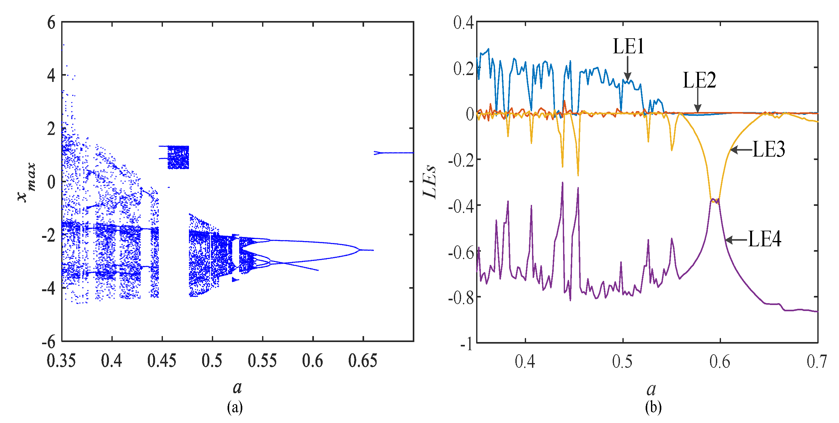
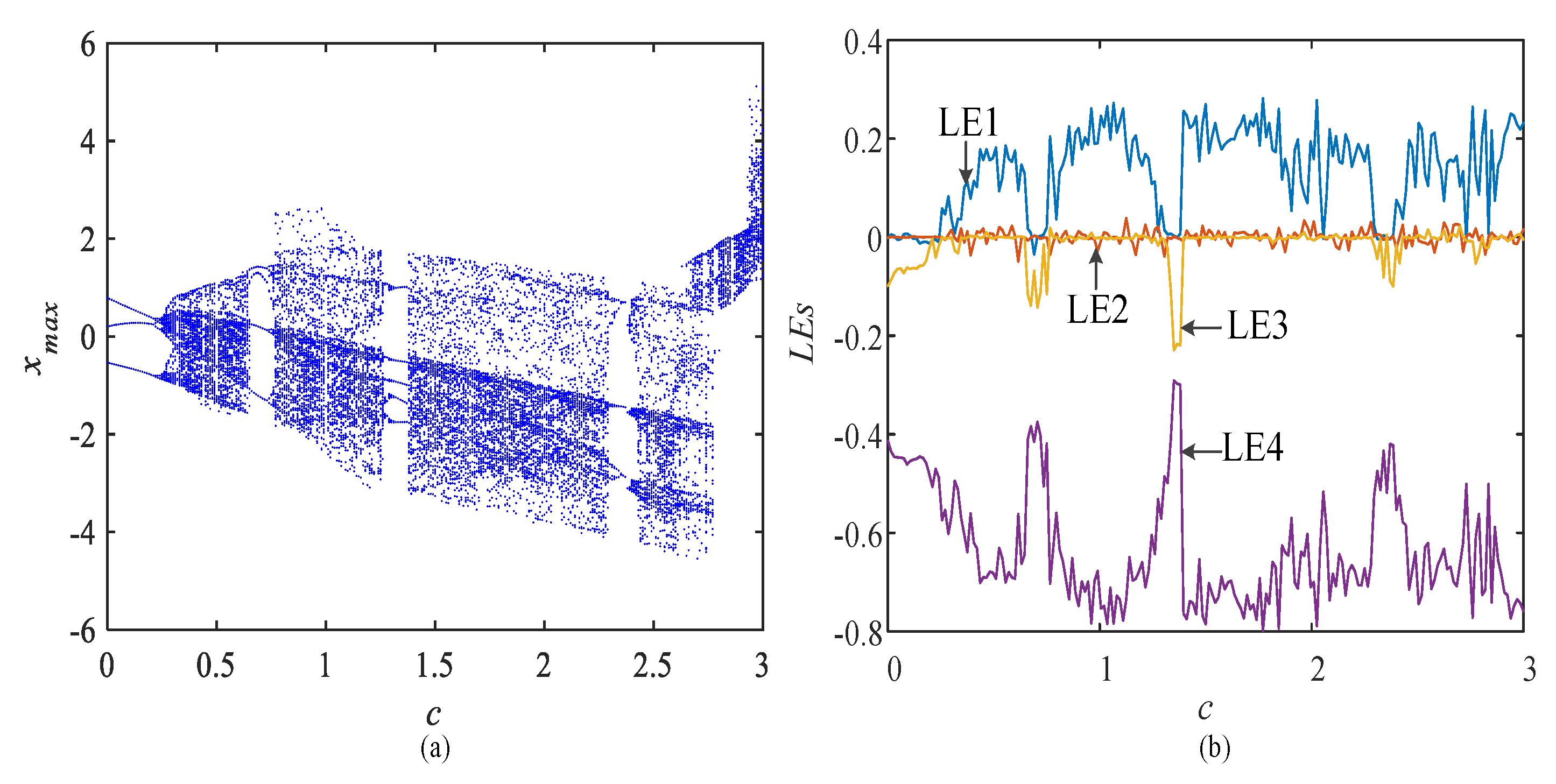
3.2. Dynamical Analysis with the Parameters

Set a as the bifurcation parameter, and set the remaining parameters as $b=2.1$, $c=2.6$, $\alpha =1.8$, $\beta =0.01$, and the order q = 0.95. When a is changed at the range [0.35, 0.7], the bifurcation diagram and its LEs are shown in Figure 4. When the control parameter a gradually increases, the system starts from the chaotic state, and several period windows appear as a increases. When a = 0.445, there is a jump in the bifurcation diagram. After the system returns to the original bifurcation path, it goes to the periodic state through the reverse period-doubling bifurcation. Figure 4b also proves the existence of these periodic windows, which verifies the above analysis.

Set $a=0.4$, while q and other parameters remain unchanged, We studied the influence of parameter c on system behavior. When c is changed at the range [0, 3], the bifurcation diagram and its LEs are shown in Figure 5. It can be seen that the system stays in the state of chaos at a large range of parameter c, except for three small period windows $c\in [0.66,0.77]$, $[1.27,1.38]$ and $[2.3,2.43].$

3.3. Dynamical Analysis with the Initial Values

Generally, chaotic systems are sensitive to initial values, but the structure of the attractor remains stable. Even if some systems are capable of coexisting attractors due to the existence of multiple stable states, the number of coexisting attractors is usually limited. Ref. [24] reported that the four-line balanced deformed Jerk system has extreme multistability. The bifurcation diagram and Lyapunov exponent spectrum of the system (8) with the initial value are plotted to analyze the behavior of the system.

Set the control parameters as $a=0.4$, $b=2.6$, $c=2.1$, $\alpha =1.8$, $\beta =0.01$, and the order $q=0.95$, and the remaining three initial values are all set to 1. Figure 6 shows the bifurcation diagram of the system changing $x_0$ and $z_0$, where $x_0$ varies at the range [−7, 5] and $z_0$ varies at the range [−3, 6]. The bifurcation behavior of the system remains unchanged when $x_0$ and $z_0$ change. So, we mainly analyze the dynamic characteristics of the system with $y_0$ and $w_0$.

Set the same system parameters and order as before, the initial conditions are assigned as $x_0=1$, $z_0=1$, $w_0=4$. $y_0$ varies at the range [−7, 9]. The bifurcation diagram and the LEs of the system (8) are shown in Figure 7. In the interval [−7, −4], the bifurcation behavior of the system is special. When the initial condition $y_0$ increases from −7, the system breaks into chaos at first through a period-doubling bifurcation. The bifurcation paths have many narrow periodic windows, and the bifurcation points corresponding to these windows form another bifurcation path with a breakpoint. Then, the system suddenly jumps to another chaotic state. As $y_0$ continues to increase, the bifurcation becomes normal. There are three obvious periodic windows, and the system quickly evolves into chaotic state again through the period-doubling bifurcation. The LEs shown in Figure 7b verify the accuracy of bifurcation diagrams.

The control parameters and order of the system (8) remain unchanged, and change the initial value to $x_0=1$, $y_0=1$, $z_0=1$; $w_0$ varies at the range [−7, 8]. The bifurcation diagram and the LEs of the system (8) are shown in Figure 8. As $w_0$ increases, it is obvious that the bifurcation diagram can be divided into five intervals of [−7,−5], (−5,−1.9], (−1.9,5], (5,6.7], (6.7,8] numbered 1–5. These five intervals have a certain degree of symmetry. In interval 1 and 5, the system evolves into a chaotic state through forward (reverse) period-doubling bifurcation. Then, the system entered interval 2 and 4 and re-evolved. In interval 3, the system is chaotic, except for a few periodic windows. LEs have more severe oscillations than Figure 7b. This is because the system state switches rapidly between periodic and chaotic. This phenomenon can be seen from interval 4 of the bifurcation diagram.

Dynamical maps based on the SE complexity [41] and the maximum Lyapunove exponents in the $y_0-w_0$ plane with $a=0.4$, $b=2.6$, $c=2.1$, $\alpha =1.8$, $\beta =0.01$ are shown in Figure 9. In Figure 9a, dark colors indicate a system is chaotic, and light colors indicate that the system may be periodic states, and white indicates divergence. The dynamic map based on the maximum Lyapunove exponent is more precise. Orange indicates the system is chaotic ($LEmax>0.03$), and yellow indicates stable resting behavior($0<LEmax<0.03$), and cyan-blue indicates periodic states and blue indicates divergence. Dynamic map based on the maximum Lyapunov exponent can distinguish the state of the system at the critical region.

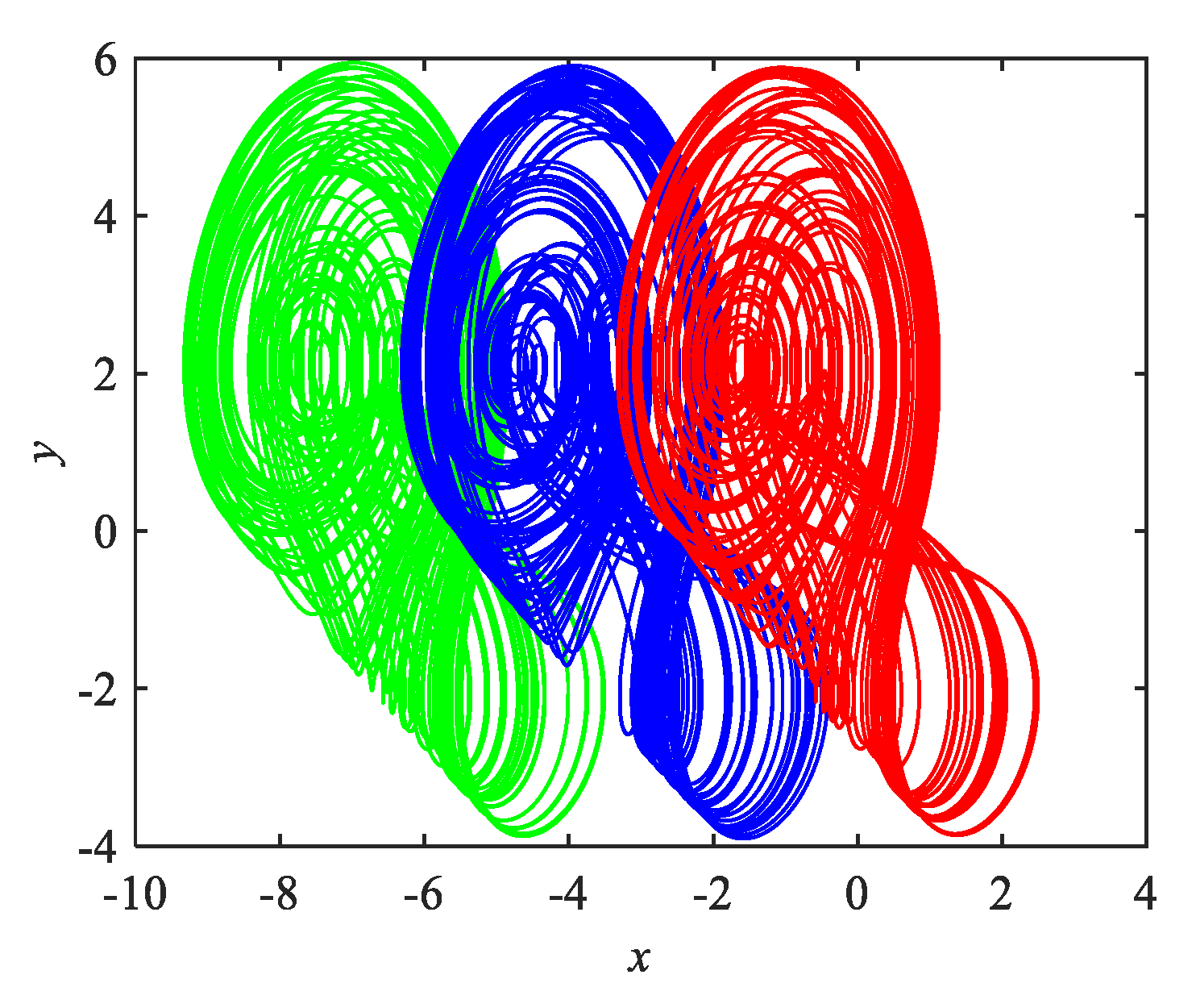
4. Multiple Coexisting Attractors of System

4.1. Multiple Coexisting Attractors and Its Digital Circuit Implementation

The control parameters and the order of system (8) remain unchanged, and we set different initial values to plot the phase diagrams. Figure 10 shows nine asymmetric coexisting attractors. In order to observe more clearly, the coexistence attractors at each initial value are separately plotted. There are four chaotic attractors with different structures and five periodic attractors. It illustrates the multiple stability of the system, and it is just a dynamic characteristic exhibited by a few sample points in the initial value space.

The hardware implementation of a chaotic system is an important method for verifying the feasibility of the system. Due to the tolerance of electronic component parameters, this increases the difficulty of using analog circuits to implement chaotic systems. However, the digital circuit implementation scheme based on the DSP platform used in this article does not have this problem. Figure 11 shows the DSP hardware connection schematic diagram. In the experiment, the IDE (Integrated Development Environment) of the DSP platform uses CCS (Code Composer Studio). We can use it to set various parameters such as system parameters and iteration step length. The initialized data are transmitted to the DSP through the communication interface for calculation, and the result is transmitted to the oscilloscope (Tektronix MDO 3104, Tektronix, Hong Kong, China) through the D/A converter (DAC8552, Texas Instruments, Dallas, TX, USA) for display.

Figure 12 shows the program flowchart. After the DSP is initialized, the various parameters of the system are set, and then iterative calculations are started. Push the result into the stack to facilitate the next calculation to call the result. The result after data processing is output through D/A. In the experiment, we set the same initial conditions as when the system has coexistence attractors. The DSP implementation hardware connection diagram is shown in Figure 13. After debugging, the system experimental phase diagram is obtained. Comparing Figure 10 and Figure 14, it can be concluded that we have successfully completed the DSP implementation.

4.2. Offset Boosting

Offset boosting control is discussed in this section. According to Ref. [27], we can generate the offset by adding a constant term after the variable that has only appeared once in the system. By observing Formula (8), we can find that the variable x satisfies the conditions for constructing offset boosting. The constant term p is added to the third dimension, so we can obtain

$$\left\{\begin{array}{c}{D}_{t_0}^{q}x=\left|y\right|-b\hfill \\ D_{t_0}^{q}y=(\alpha +3\beta w^2)z\hfill \\ D_{t_0}^{q}z=|x+p|-y-az-c\hfill \\ D_{t_0}^{q}w=z\hfill \end{array}\right..$$

(16)

Set the system parameters and order to remain the same as during characteristic analysis, the initial conditions [1, 1, 1, 4], and the offset parameter p are set to −3, 0, 3. The offset boosting phenomenon is illustrated in Figure 15. After the offset boosting control is applied, the system has richer dynamic behavior under certain initial values. Only change the initial conditions to [1, 1, 1, 5.5] without changing other conditions. Figure 16 shows the offset boosting phenomenon under this condition. It shows the boosting phenomenon of three different states under the same initial value. When p = 3, 2, 1, 0, the system remains in a chaotic state for boosting. When p = −1, −1.2, −1.4, −1.6, the system remains a double-periodic orbit for boosting. When p = 3, −4, −5, −6, the system remains a single-periodic orbit for boosting.

5. Conclusions

In this paper, many analysis methods are used to analyze the dynamic characteristics of this fractional-order menristor-based hypogenetic jerk system, such as a phase diagram, bifurcation diagram, and Lyapunov exponent spectrum. DSP technology is used to successfully verify the feasibility of the system. It is found that the system not only has rich dynamic characteristics with the change of the order and system parameters, but also has a complete period-doubling bifurcation path from single-cycle to multi-cycle with the change in initial values. A change in the bifurcation path implies a change in the structure of the attractor. Through phase diagram analysis, at least nine coexisting attractors were found. The control and application of this fractional-order menristor-based hypogenetic jerk system will be studied next.

References

1. Luo, J.; Xu, X.; Ding, Y.; Yuan, Y.; Yang, B.; Sun, K.; Yin, L. Application of a memristor-based oscillator to weak signal detecbtion. Eur. Phys. J. Plus 2018, 133, 239. [Google Scholar] [CrossRef]
2. Hua, Z.; Zhou, Y.; Huang, H. Cosine-transform-based chaotic system for image encryption. Inf. Sci. 2019, 480, 403–419. [Google Scholar] [CrossRef]
3. Ye, X.; Mou, J.; Luo, C.; Wang, Z. Dynamics analysis of Wienbridge hyperchaotic memristive circuit system. Nonlinear Dyn. 2018, 92, 923–933. [Google Scholar] [CrossRef]
4. Wang, X.; Wang, S.; Zhang, Y.; Luo, C. A one-time pad color image cryptosystem based on SHA-3 and multiple chaotic systems. Opt. Lasers Eng. 2018, 103, 1–8. [Google Scholar] [CrossRef]
5. Mou, J.; Sun, K.; Ruan, J.; He, S. A nonlinear circuit with two memcapacitors. Nonlinear Dyn. 2016, 86, 1–10. [Google Scholar] [CrossRef]
6. Wang, G.; Zang, S.; Wang, X.; Yuan, F.; Iu, H.H.-C. Memcapacitor model and its application in chaotic oscillator with memristor. Chaos 2017, 27, 013110. [Google Scholar] [CrossRef]
7. Bao, H.; Wang, N.; Wu, H.; Song, Z.; Bao, B. Bi-stability in an improved memristor-based third-order Wien-bridge oscillator. IETE Tech. Rev. 2019, 36, 109–116. [Google Scholar] [CrossRef]
8. Chua, L. Memristor-the missing circuit element. IEEE Trans. Circuit Theory 1971, 18, 507–509. [Google Scholar] [CrossRef]
9. Strukov, D.B.; Snider, G.S.; Stewart, D.R.; Williams, R.S. The missing memristor found. Nature 2008, 453, 80–83. [Google Scholar] [CrossRef]
10. Yalagala, B.; Khandelwal, S.; Deepika, J.; Badhulika, S. Wirelessly destructible MgO-PVP-Graphene composite based flexible transient memristor for security applications. Mat. Sci. Semicon. Proc. 2019, 104, 104673. [Google Scholar] [CrossRef]
11. Wang, W.; Jia, X.; Luo, X.; Kurths, J.; Yuan, M. Fixed-time synchronization control of memristive MAM neural networks with mixed delays and application in chaotic secure communication. Chaos Soliton Fract. 2019, 126, 85–96. [Google Scholar] [CrossRef]
12. Zhang, W.; Cao, J.; Wu, R.; Chen, D.; Alsaadi, F.E. Novel results on projective synchronization of fractional-order neural networks with multiple time delays. Chaos Soliton Fract. 2018, 117, 76–83. [Google Scholar] [CrossRef]
13. Lunelli, L.; Collini, C.; Jimenez-Garduño, A.; Roncador, A.; Giusti, G.; Verucchi, R.; Pasquardini, L.; Iannotta, S.; Macchi, P.; Lorenzelli, L.; et al. Prototyping a memristive-based device to analyze neuronal excitability. Biophys. Chem. 2019, 253, 106212. [Google Scholar] [CrossRef]
14. Sun, J.; Yang, Q.; Wang, Y. Dynamical analysis of novel memristor chaotic system and DNA encryption application. IJST-T Electr. Eng. 2020, 44, 449–460. [Google Scholar] [CrossRef]
15. Rajagopal, K.; Guessas, L.; Karthikeyan, A.; Srinivasan, A.; Adam, G. Fractional-order memristor no equilibrium chaotic system with its adaptive sliding mode synchronization and genetically optimized fractional order PID synchronization. Complexity 2017, 2017, 1–19. [Google Scholar] [CrossRef] [Green Version]
16. Chen, M.; Feng, Y.; Bao, H.; Bao, B.; Wu, H.; Xu, Q. Hybrid state variable incremental integral for reconstructing extreme multistability in memristive jerk system with cubic nonlinearity. Complexity 2019, 2019, 1–16. [Google Scholar] [CrossRef] [Green Version]
17. Xu, B.; Wang, G.; Iu, H.H.-C.; Yu, S.; Yuan, F. A memristor-meminductor-based chaotic system with abundant dynamical behaviors. Nonlinear Dyn. 2019, 96, 765–788. [Google Scholar] [CrossRef]
18. Sadecki, J.; Marszalek, W. Complex oscillations and two-parameter bifurcations of a memristive circuit with diode bridge rectifier. Microelectron. J. 2019, 93, 104636. [Google Scholar] [CrossRef]
19. Rajagopal, K.; Li, C.; Nazarimehr, F.; Karthikeyan, A.; Duraisamy, P.; Jafari, S. Chaotic dynamics of modified wien bridge oscillator with fractional order memristor. Radioengineering 2019, 27, 165–174. [Google Scholar] [CrossRef]
20. Ruan, J.; Sun, K.; Mou, J.; He, S.; Zhang, L. Fractional-order simplest memristor-based chaotic circuit with new derivative. Eur. Phys. J. Plus 2018, 133, 3. [Google Scholar] [CrossRef]
21. Mou, J.; Sun, K.; Wang, H.; Ruan, J. Characteristic analysis of fractional-order 4D hyperchaotic memristive circuit. Math. Probl. Eng. 2017, 2017, 2313768. [Google Scholar] [CrossRef] [Green Version]
22. Li, R.; Huang, D. Stability analysis and synchronization application for a 4D fractional-order system with infinite equilibria. Phys. Scripta 2020, 95, 015202. [Google Scholar] [CrossRef]
23. Chen, C.; Chen, J.; Bao, H.; Chen, M.; Bao, B. Coexisting multi-stable patterns in memristor synapse-coupled Hopfield neural network with two neurons. Nonlinear Dyn. 2019, 95, 3385–3399. [Google Scholar] [CrossRef]
24. Bao, H.; Wang, N.; Bao, B.; Chen, M.; Jin, P.; Wang, G. Initial condition-dependent dynamics and transient period in memristor-based hypogenetic jerk system with four line equilibria. Commun. Nonlinear Sci. 2018, 57, 264–275. [Google Scholar] [CrossRef]
25. Wan, P.; Sun, D.; Zhao, M.; Wan, L.; Jin, S. Multistability and attraction basins of discrete-time neural networks with nonmonotonic piecewise linear activation functions. Neural Netw. 2020, 122, 231–238. [Google Scholar] [CrossRef]
26. Chen, M.; Sun, M.; Bao, H.; Hu, Y.; Bao, B. Flux-charge analysis of two-memristor-based chua’s circuit: Dimensionality decreasing model for detecting extreme multistability. IEEE T Ind. Electron. 2020, 67, 2197–2206. [Google Scholar] [CrossRef]
27. Li, C.; Sprott, J.C. Variable-boostable chaotic flows. Optik 2016, 127, 10389–10398. [Google Scholar] [CrossRef]
28. Bayani, A.; Rajagopal, K.; Khalaf, A.J.M.; Jafari, S.; Leutcho, G.; Kengne, J. Dynamical analysis of a new multistable chaotic system with hidden attractor: Antimonotonicity, coexisting multiple attractors, and offset boosting. Phys. Lett. A 2019, 383, 1450–1456. [Google Scholar] [CrossRef]
29. Li, C.; Lei, T.; Wang, X.; Chen, G. Dynamics editing based on offset boosting. Chaos 2020, 30, 063124. [Google Scholar] [CrossRef] [PubMed]
30. Li, H.; Yang, Y.; Li, W.; He, S.; Li, C. Extremely rich dynamics in a memristor-based chaotic system. Eur. Phys. J. Plus 2020, 135, 579. [Google Scholar] [CrossRef]
31. Zhang, S.; Zheng, J.; Wang, X.; Zeng, Z.; He, S. Initial offset boosting coexisting attractors in memristive multi-double-scroll hopfield neural network. Nonlinear Dyn. 2020, 102, 2821–2841. [Google Scholar] [CrossRef]
32. Yu, F.; Liu, L.; Shen, H.; Zhang, Z.; Huang, Y.; Cai, S.; Deng, Z.; Wan, Q. Multistability analysis, coexisting multiple attractors, and FPGA implementation of Yu-Wang four-wing chaotic system. Math. Probl. Eng. 2020, 2020, 1–16. [Google Scholar] [CrossRef]
33. Ding, D.; Shan, X.; Jun, L.; Hu, Y.; Yang, Z.; Ding, L. Initial boosting phenomenon of a fractional-order hyperchaotic system based on dual memristors. Mod. Phys. Lett. B 2020, 34, 2050191. [Google Scholar] [CrossRef]
34. Tamba, V.K.; Kom, G.H.; Kingni, S.T.; Mboupda Pone, J.R.; Fotsin, H.B. Analysis and electronic circuit implementation of an integer- and fractional-order four-dimensional chaotic system with offset boosting and hidden attractors. Eur. Phys. J.Spec. Top. 2020, 229, 1211–1230. [Google Scholar] [CrossRef]
35. He, S.; Sun, K.; Wang, H. Solution of the fractional-order chaotic system based on Adomian decomposition algorithm and its complexity analysis. Acta Phys. Sin. Ed. 2014, 63, 030502. [Google Scholar]
36. Ye, X.; Wang, X.; Mou, J.; Yan, X.; Xian, Y. Characteristic analysis of the fractional-order hyperchaotic memristive circuit based on the Wien bridge oscillator. Eur. Phys. J. Plus 2018, 133, 516. [Google Scholar] [CrossRef]
37. Yang, F.; Li, P. Characteristics analysis of the fractional-order chaotic memristive circuit based on Chua’s circuit. Mob. Netw. Appl. 2019, 5, 1–9. [Google Scholar] [CrossRef]
38. Yang, F.; Mou, J.; Ma, C.; Cao, Y. Dynamic analysis of an improper fractional-order laser chaotic system and its image encryption application. Opt. Laser Eng. 2020, 129, 106031. [Google Scholar] [CrossRef]
39. He, S.; Sun, K.; Wang, H. Complexity analysis and DSP implementation of the fractional-order Lorenz hyperchaotic system. Entropy 2015, 17, 8299–8311. [Google Scholar] [CrossRef] [Green Version]
40. He, S.; Sun, K.; Wang, H. Solution and dynamics analysis of a fractional-order hyperchaotic system. Math. Methods Appl. Sci. 2016, 39, 2965–2973. [Google Scholar] [CrossRef]
41. Sun, K.H.; He, S.B.; He, Y.; Yin, L.Z. Complexity analysis of chaotic pseudo-random sequences based on spectral entropy algorithm. Acta. Phys. Sin. Ed. 2013, 62, 010501. [Google Scholar]
Figure 1. Phase diagrams of the system: (a) x y plane; (b) z w plane.
Electronics 10 00841 g001
Figure 2. Phase diagrams with different q: (a) q = 0.21; (b) q = 0.35; (c) q = 0.5; (d) q = 0.52; (e) q = 0.6; (f) q = 0.9.
Electronics 10 00841 g002
Figure 3. Dynamics with q change: (a) bifurcation diagram, (b) Lyapunov exponents.
Electronics 10 00841 g003
Figure 4. Dynamics with a change: (a) bifurcation diagram; (b) Lyapunov exponents.
Electronics 10 00841 g004
Figure 5. Dynamics with c change: (a) bifurcation diagram; (b) Lyapunov exponents.
Electronics 10 00841 g005
Figure 6. Bifurcation diagrams with x 0 and z 0 change: (a) x 0 change; (b) z 0 change.
Electronics 10 00841 g006
Figure 7. Dynamics with y 0 change: (a) bifurcation diagram; (b) Lyapunov exponents.
Electronics 10 00841 g007
Figure 8. Dynamics with w 0 change: (a) bifurcation diagram; (b) Lyapunov exponents.
Electronics 10 00841 g008
Figure 9. Dynamic maps in y 0 w 0 : (a) based on SE complexity; (b) based on maximum Lyapunov exponent.
Electronics 10 00841 g009
Figure 10. Multiple coexisting attractors with different initial values.
Electronics 10 00841 g010
Figure 11. The digital signal processor (DSP) hardware connection schematic diagram of fractional-order memristor-based hypogenetic jerk system.
Electronics 10 00841 g011
Figure 12. Flowchart for DSP implementation program.
Electronics 10 00841 g012
Figure 13. The DSP implementation hardware connection diagram.
Electronics 10 00841 g013
Figure 14. Multiple coexisting attractor with different initial values: (a) (1 1 1 6); (b) (1 1 1 −2.7); (c) (1 1 1 7); (d) (1 1 1 2); (e) (1 1 1 1); (f) (1 1 1 −6); (g) (1 1 1 −2); (h) (1 1 1 −4); (i) (1 1 1 8).
Electronics 10 00841 g014
Figure 15. Offset boosting with control parameter p. p = 3 (green), p = 0 (blue), p = −3 (red).
Electronics 10 00841 g015
Figure 16. Offset boosting with control parameter p. (a) p = 3, 2, 1, 0; (b) p = −1, −1.2, −1.4, −1.6; (c) p = −3, −4, −5, −6.
Electronics 10 00841 g016
Publisher’s Note: MDPI stays neutral with regard to jurisdictional claims in published maps and institutional affiliations.