Article

Battery Powered Inductive Welding System for Electrofusion Joints in Optical Fiber Microducts

Department of Electronics Design, Mid Sweden University, 851 70 Sundsvall, Sweden
*
Author to whom correspondence should be addressed.
Electronics 2021, 10(6), 743; https://doi.org/10.3390/electronics10060743
Submission received: 25 December 2020 / Revised: 28 February 2021 / Accepted: 2 March 2021 / Published: 21 March 2021
(This article belongs to the Section Power Electronics)

Abstract

:
Optical fiber microducts are joined together by mechanical joints. These mechanical joints are bulky, require more space per joint, and are prone to air pressure leakage and water seepage during service. A battery powered electrofusion welding system with a resistive-type joint has been recently developed to replace mechanical joints. These resistive-type electrofusion joints require physical connectors for power input. Due to a different installation environment, the power input connectors of resistive optical fiber microduct joints may corrode over time. This corrosion of connectors will eventually cause water seepage or air pressure leakage in the long run. Moreover, due to connector corrosion, resistive-type optical fiber microduct joints cannot be re-heated in future if the need arises. In this study, an inductively coupled electrofusion-type joint was proposed and investigated. This inductive-type electrofusion joint is not prone to long-term corrosion risk, due to the absence of power connectors. Inductive-type electrofusion joints can be re-heated again for resealing or removal in the long run, as no metal part is exposed to the environment. The battery powered inductive welding system can be easily powered with a 38 volts 160 watt-hour battery. The inductive-type electrofusion joint was welded within one second, and passed a 300-newton pull strength test and a 10-bar air pressure leakage test. It was demonstrated that the power input requirement for inductive electrofusion joints is 64% higher than that of resistive electrofusion joints. However, these inductive joints are relatively easy to manufacture, inexpensive, have no air leakage, and no water seepage risk in highly corrosive environments.

1. Introduction

Optical fiber communication is increasing at a pace greater than ever. Due to recent demands of fiber to the home (FTTH), cable-TV, internet, and IoT applications, the upgrade and new installation of optical fibers are in greater demand than ever. Optical fiber cables are installed inside polymer conduits known as microducts. These microducts are buried underground before the actual optical fiber cable installation by various methods, i.e., mechanical pulling, air blowing, and water floating [1]. Due to field requirements, these microducts require a joint for the installation of optical fiber cables. At present, mechanical joints are used for joining two optical fiber microducts. A type of mechanical joint is shown in Figure 1a. Mechanical joints are bulky and have poor water sealing capabilities. To protect against water and moisture, an extra water sealing jacket is used, as shown in Figure 1b. This water jacket provides IP68 protection against moisture and water seepage. Water seepage is considered a major problem in modern optical fiber communication systems. Frozen water inside ducts results in communication signal attenuations, and may cause duct rupture or undesirable bending in the optical fiber cables installed inside the ducts [2]. The air pressure sustaining capability of mechanical joints is principally dependent upon O-rings. Experience has shown that the mechanical joints leak at air pressures lower than 1 bar [3]. The normal installation air pressure in blown optical fiber is 15 bars for a 14.0 mm microduct. With air leakage at 1 bar, the present mechanical joints cannot be installed up to maximum attainable length with many joints along the way.
Without any type of joint, optical fibers can be extended to 800 m, or even more [4]. Moreover, mechanical joints need to be cut at different lengths in multi-microduct installations to keep the overall diameter of the multiduct joints small. A straight duct, as shown in Figure 1c, is used to join the multiduct at different lengths. Mechanical joints can be joined with a click action which requires about one second. These mechanical joints have an inbuilt metallic lock ring that locks onto the surface of microducts, as shown in Figure 1d. Mechanical joints are rated to withstand more than 200 newtons pull strength, and with no physical damage up to 25 bars of air pressure. These joints have inbuilt O-rings on each side to provide the main protection against air pressure leakage and water seepage. Mechanical joints are also rated to protect against air pressure leakage up to 0.5 bars.

Previous Work

The optical fiber microduct is made up of high density polyethylene (HDPE). HDPE is a type of thermoplastic, which is used in water, sewage, gas, and the delivery of chemicals in industry [5]. HDPE pipes are thermoelectrically welded in these engineering applications and to do so, electrofusion (EF) welding is one such popular method [6]. In electrofusion welding, a cylindrical shaped HDPE or MDPE barrel, with copper heating wire inside, is electrically powered for a specific time to produce heat by the Joule effect. When the temperature at the interface rises above the polymer’s melting temperature, the molten polymer flows and welds the two interfaces, as shown in Figure 2. Electrofusion welding is an almost five-decade-old method of joining HDPE pipes [6]. A lot of research has been carried out into the electrofusion welding of water, gas, and sewage transport systems. A comprehensive amount of data has been collected about the temperature requirement of the interface [7] and thermal modeling of EF joints [8]. An extensive amount of research has also been done on the failure mechanism of electrofusion joints [9]. Other than that, the strength of these electrofusion joints and the effect of UV exposure and oxidation have also been briefly discussed [10]. The minimum welding time of electrofusion joints was found to be of 32 s for 25.0 mm EF joints in the water and gas industries [11].
The main challenge of the electrofusion welding of optical fiber ducts is the very short welding time, i.e., 1 s to compare with the mechanical joints in terms of time per joint. The other challenges for electrofusion welding in optical fiber microducts are withstanding a pull strength of 200 newtons, no air pressure leakage at 15 bars, and no water seepage. The authors have previously developed an LTspice electrothermal model of heat generation and propagation inside optical fiber microducts [12]. The Ltspice electrothermal model was developed using an electrical to thermal analogy [13]. In the developed Ltspice electrothermal model, the thermal parameters were extracted using the thermal properties and the geometric shapes of the materials [14]. The calculated thermal parameters were connected in a Cauer thermal model configuration, where each RC node represents the temperature at the corresponding outer layer of the LDPE shell [15]. The developed LTspice electrothermal model was utilized to develop a battery powered electrofusion welding system with a resistive type optical fiber electrofusion joint (ROFEF) joint [3]. In Akram et al. [3], it was shown that the battery powered electrofusion welding of two optical fiber microducts could be achieved with a power input of 167.74 joules, and it could withstand 300 newtons pull strength and 10 bars of air pressure, showing no signs of air leakage and water seepage. The developed LTspice welding model [3] is reproduced here in Figure 3a. The model utilized a capacitor bank of 0.056 farads and a PWM charge–discharge cycle to power the ROFEF joint. The developed ROFEF joint is shown in Figure 3b. The developed controller board for welding of the ROFEF joint is shown in Figure 3c. Three different duty cycles of 70%, 50%, and 30% of PWM were used to model, simulate, and validate the results of the welding of the ROFEF joint. The results of the 50% and 70% duty cycles were able to pass the conformity test with the mechanical joint specification. The welded ROFEF joints were able to withstand 300 newtons of pull strength and 10 bars of air pressure tests without any physical damage or air leakage. It was shown that the ROFEF joint can replace mechanical joints in the future. The other advantages of ROFEF joints compared to mechanical joints are that they are compact, smaller in size, less complex than mechanical joints, and almost 2000+ joints can be welded with a 38 volts 160 watt-hour battery. However, the ROFEF joint requires a physical connector to transfer power. Some salient features of the previous study by Akram et al. [3] are mentioned below:
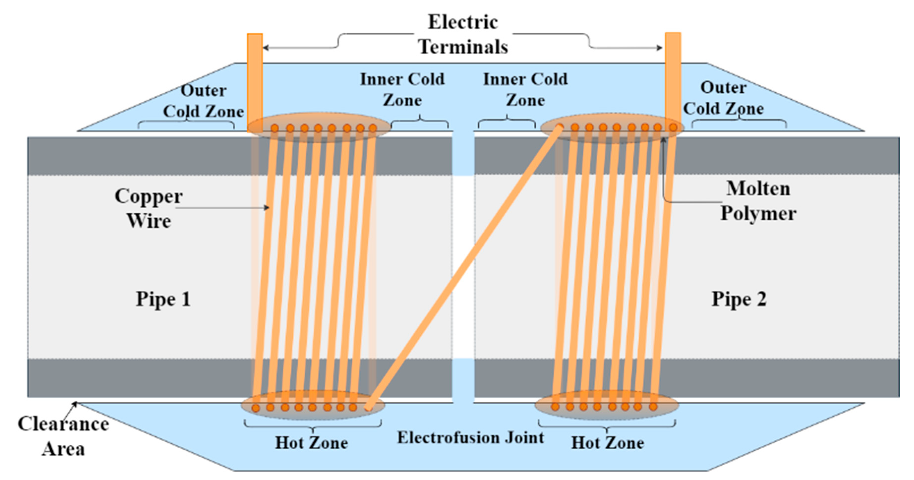
  • A thermal model based on thermal to electrical analogy was developed and utilized to estimate the power input required and resulting temperature inside a ROFEF joint.
  • It is possible to achieve a temperature of 190 °C within one second with a 38 volt, 160 watt-hour battery with the help of PWM charge–discharge cycles.
  • It can weld two optical fiber microducts within one second.
  • The strength of the ROFEF joint can withstand 300 newtons of pull strength and 10 bars of air pressure without air pressure leakage or physical damage.
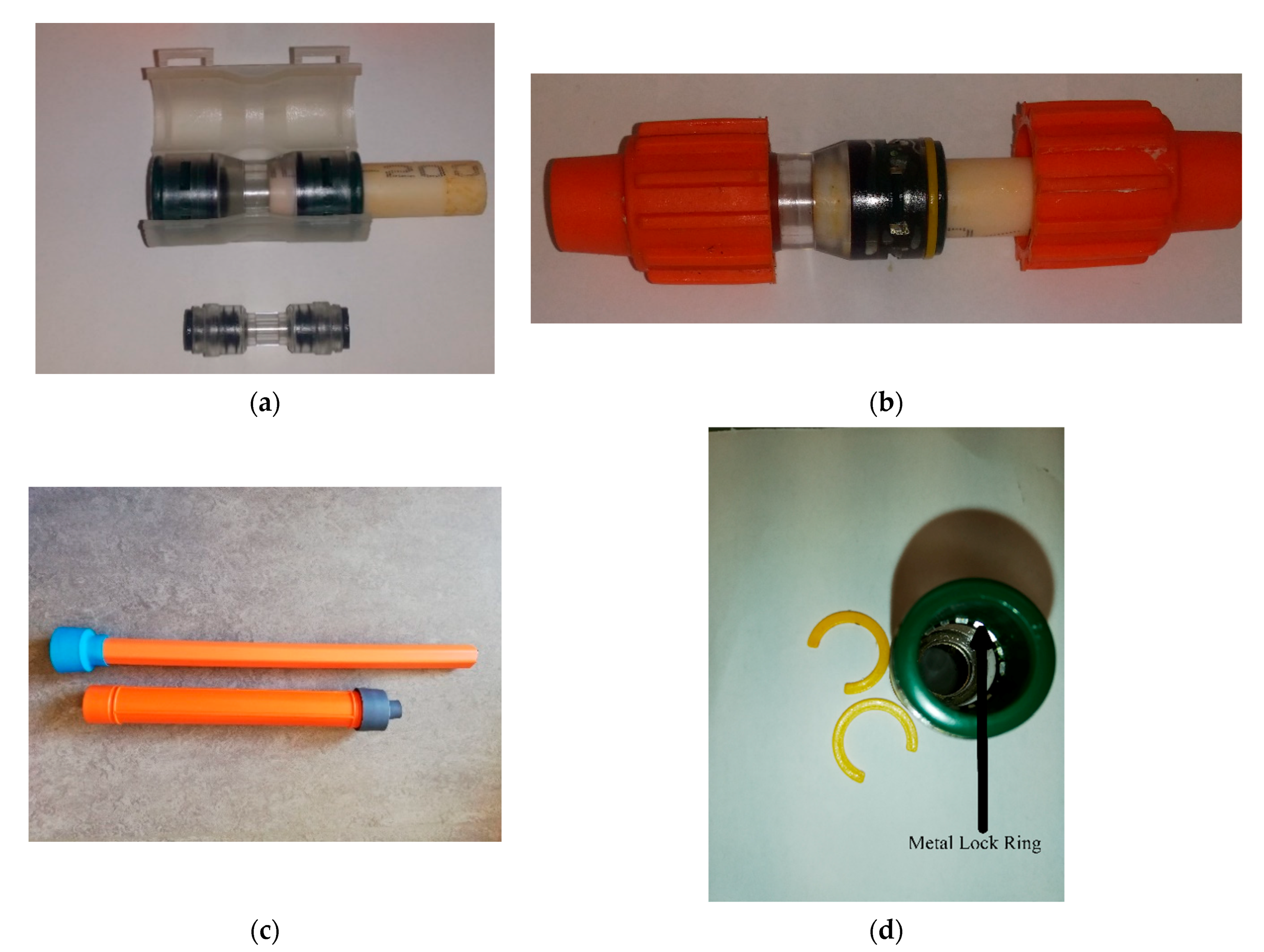
  • The ROFEF joint requires a physical connector for connection and transfer of battery power to the ROFEF joint.
In the optical fiber industry, sometimes optic fiber microducts are installed through sewage or drain pipes [16]. This practice requires no need to dig a trench or micro trench and thus avoids third party liabilities [16]. In these environments, whether they are chemical corrosion prone or a natural environment, the copper connector rings on ROFEF joints may corrode very quickly, and the protection level is reduced considerably. Moreover, consequently, the ROFEF joints may become prone to water seepage. Nowadays, it has also become a normal practice in the optical fiber industry to overblow [17] an optical fiber cable in an already available microduct, with some optical fiber pre-installed or blown earlier. In these installation environments, the ROFEF joints impose a leakage risk and thus cannot be utilized efficiently. In a mechanical optical fiber joint (Figure 1d), the metallic lock ring has no protection from corrosion. Thus, when this metallic ring corrodes, the mechanical joint will open. In recent years, in order to overcome this problem, optical fiber and telecommunication industry vendors have developed metal-free, purely plastic based joints. These metal-free joints are bulkier than normal mechanical joints, they have relatively lower pull strength due to missing metallic lock rings, and they have better water seepage protection due to bulky and thick O-rings. However, they are rated at only 0.5 bars for air pressure leakage.
The study presented in this article explores the possibility of contactless, inductive power transfer to the inductive-type optical fiber electrofusion joint (IOFEF) joint so that they can be used in a highly corrosive environment, and re-welded or de-welded in the future. Doing so is impossible with ROFEF joints, which may lose their connectors to corrosion, and are deemed prone to air pressure leakage and water seepage in the long run. To remove the connectors of ROFEF joints and to protect the joint against corrosion, an IOFEF joint is developed and evaluated in this article. A 38 volt, 160 watt-hour battery can power the non-contact welding system, and has the same level of strength and quality as the ROFEF joints. In this study, a rather simpler induction circuit was utilized to investigate the basic inductive welding of an optical fiber microduct joint. The results show that despite the increased power consumption due to losses inside the induction circuit and lower coupling coefficient between the work coil and IOFEF joint, it is still possible to weld a non-contact IOFEF joint with a 38 volts 160 watt-hour battery. The welding time is 1 s and these inductively welded joints can easily withstand a pull strength of 300 newtons and air pressure of 10 bars, without any air leakage and water seepage for much longer periods in highly corrosive environments.

2. Methods

2.1. Design and Development of a IOFEF Joint and Inductive Work Coil

For the development of a IOFEF joint, small modifications are made to the ROFEF joint by connecting both sides of the joule heating wire and removing the power connector rings. In this way, a completely diffused joule heating wire inside an IOFEF joint is possible, which will have no contact with the outer environment, for protection against corrosion. The IOFEF joint will have the same winding sequence and the number of wire turns as was used for the ROFEF joint. A total of 14 turns of 0.1 mm insulated copper wire was wound in a group of 6 + 1 turn on one side and the other side. The joule heating wire turns started with 6 turns of the first heating zone on the first side, and then 1 turn of the second heating zone on the first side. Then again 6 turns from the second heating zone and 1 turn to the middle of IOFEF joint. Similarly, but in an opposite winding sequence to the first side, 1 turn from the middle of the IOFEF joint to the 6 turns second heating zone on the second side and 1 turn again to the 6 turns first heating zone on the second side. In this way, two heating zones were created on each side of an IOFEF joint. The splitting of a single heating zone into two heating zones on each side resulted in better welding strength and leakage protection in the study of Akram et al. [3]. The sample sketch and layer distribution are shown in Figure 4. In Figure 4, it is demonstrated how each heating zone is divided into layers, and the relative thickness of each layer for calculation of thermal parameters Rth and Cth can be seen. The calculation and estimation of thermal parameters have been thoroughly described in Akram et al. [3]. The thermal parameters calculated in Akram et al. [3] and reproduced here in Figure 3a can be directly used for an inductive welding system, as they are equal and similar to each other in the ROFEF joint and the IOFEF joint.
For efficient power transfer to the IOFEF joint, a proper work coil design is crucial. There are many possibilities of work coil design that can efficiently transfer the power to the IOFEF joint.
However, due to the geometrical shape and orientation of the joule heating wire, only a helical style work coil is practical for an efficient transfer of power. For this purpose, a work coil consisting of 17 turns in total, with a 2.0 mm Litz wire consisting of 1400 copper wires of 0.04 mm diameter each, was used. The work coil design is shown in Figure 5. However, this work coil design faces a practical restraint regarding the insertion and removal of the IOFEF joint inside it. It is possible to make a complete work coil assembly by cutting each turn from the middle and then designing a custom connector for each coil turn to deliver the power to the IOFEF joint. This type of work coil assembly can be opened for insertion of the IOFEF joint and removal after welding. The complete development of the mechanical construction of the work coil assembly is a part of mechanical design problem, where the IOFEF joint welding will be successful in terms of time, power input, pull strength, and air pressure test. There are many other possibilities of inductive coupling which may not require this helical type work coil and helical type joule heating wire in a IOFEF joint. Thus the mechanical assembly of the work coil is omitted in this study.

2.2. Design of ZVS Inductive Power Transfer Circuit

The electrical circuit of a non-contact welding system can be developed in many ways, depending upon the switching technique [18], circuit topology [19], and power requirements [20]. For the battery powered non-contact welding system, a zero voltage switching (ZVS) circuit, shown in Figure 6, was utilized. This circuit works on a hard zero voltage switching for minimum switching losses. The chosen circuit is uncomplicated, requires the lowest number of components, and is very simple to build. For efficient modeling of an inductive circuit in LTspice, the inductive parameters of the work coil, L1, L2, and inductor L3, a Bode 100 impedance analyzer was used. Table 1 below, gives the results of parameter extraction for L1, L2, and L3, which are embedded in the circuit of Figure 6.

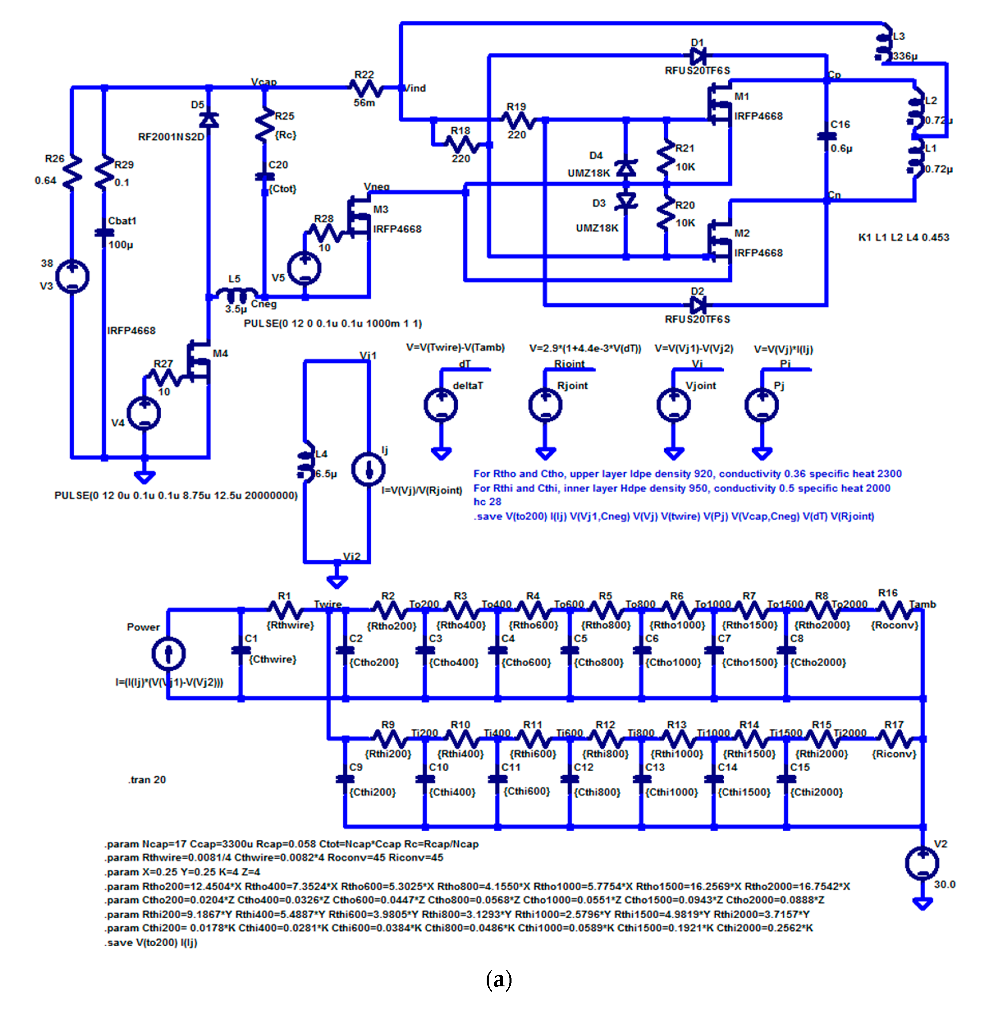
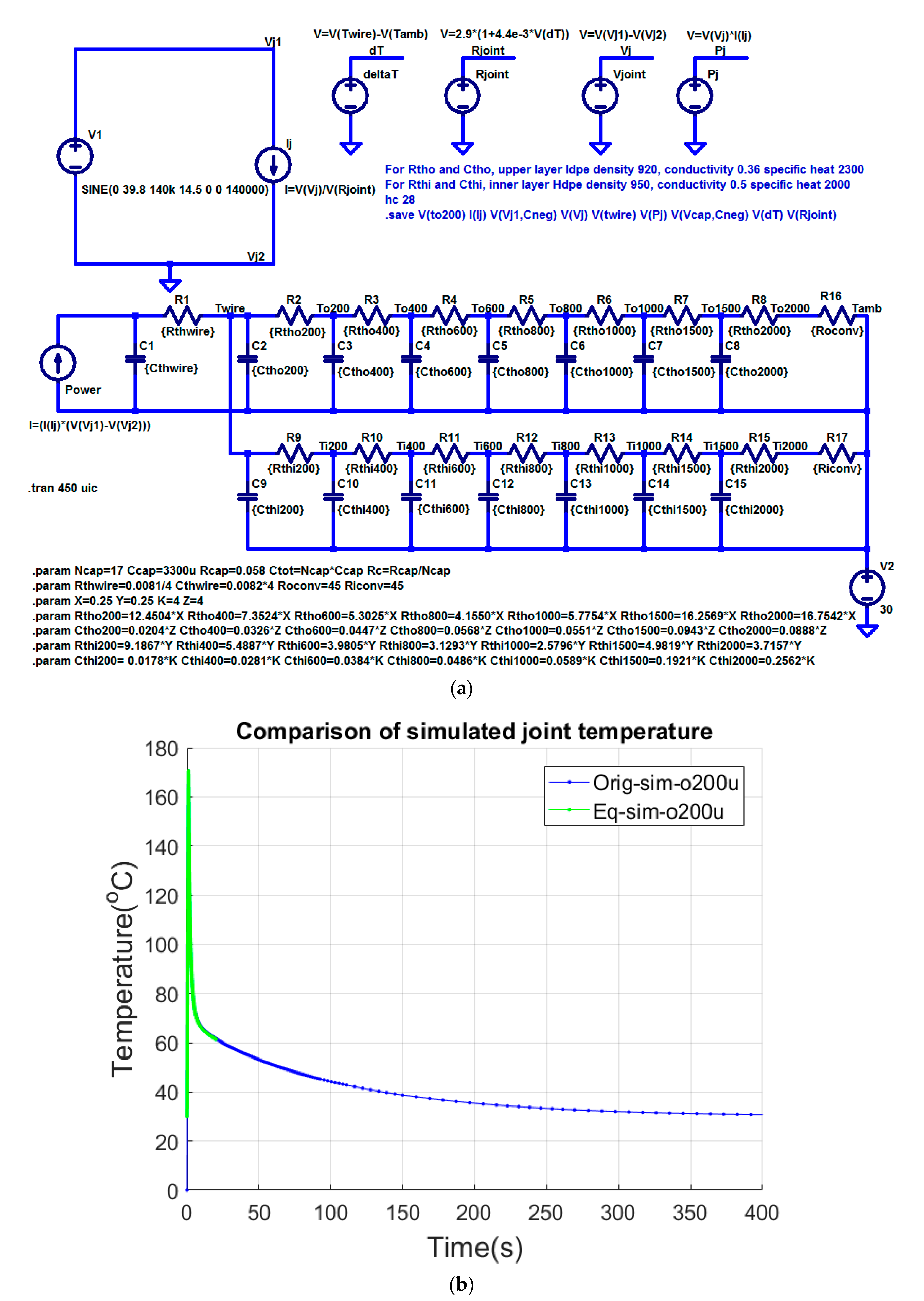
2.3. Development of the Inductive Non-Contact LTspice Welding Model

After the IOFEF joint and its driving circuit was designed, it was necessary to model the complete welding system. For control of the power input to the IOFEF joint, an already developed controller board, Figure 3c, was used. In this way, it had the flexibility of controlling the desired power level and the advantage of a resistive bank to deposit more energy in a short time interval, which can be harvested as was described in Akram et al. [3]. For this purpose, the circuits shown in Figure 3a and Figure 6 can be combined to give a complete simulation model, as shown in Figure 7a.
The coupling factor K of inductive coupling is defined as
K = L o p e n L s h o r t L o p e n
where L o p e n and L s h o r t are the open circuit and short circuit inductance of the work coil measured when the IOFEF joint is open and a short circuit inside the work coil. For measurement of the K factor, the work coil inductance was measured with a Bode 100 impedance analyzer. The values of L o p e n and L s h o r t were 1.85 µH and 1.47 µH, respectively, and thus the coupling factor (K) was calculated to be 0.453.
By simulating the LTspice model of Figure 7a, the current through the IOFEF joint and the resulting temperature inside the first outer layer, Lo200, of the IOFEF joint were calculated, and are shown in Figure 7b,c respectively. The simulation time of the LTspice model in Figure 7a was about 24 h for 20 s of simulated response. For a faster simulation time of the temperature to show the complete cooling curve, the LTspice welding model of Figure 7a can be reduced to Figure 8a. The temperature simulation of 400 s of Ltspice equivalent model of Figure 8a is shown in Figure 8b, along with the simulation result of Figure 7c.

2.4. Validation of Simulated Results and Sample Preparation for IOFEF Joint Welding

Validation of the simulated data could be done by the IOFEF joint sample, and then measuring the parameters such as power input to the IOFEF joint, resonance frequency, and resulting temperature at layer Lo200.

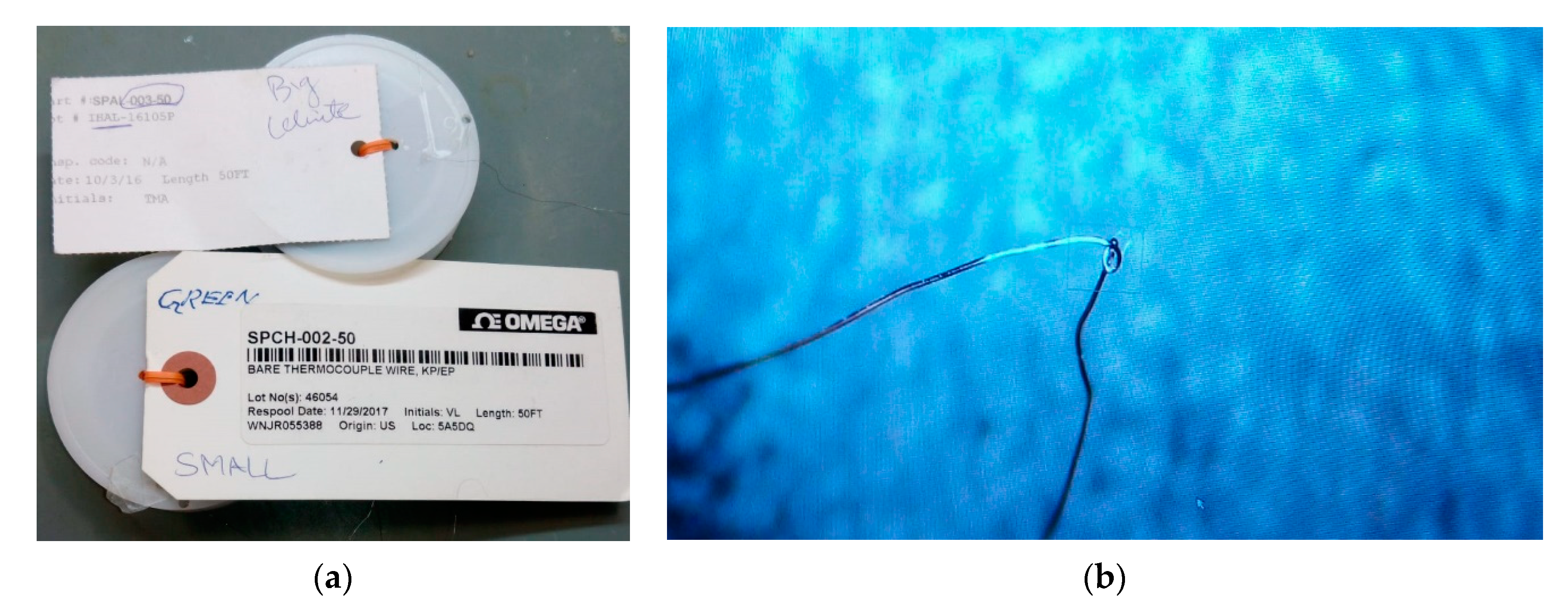
2.4.1. Custom Fabrication of a 50 µm K-Type Thermocouple

For this study, custom built 50 μm K-type thermocouples were used for validation. For custom fabrication of the K-type thermocouples, off the shelf 200 μm, K-type thermocouples were cut at the bead end and 50 µm wires of Chromel SPCH 0020-50 and Alumel SPAL 002-50 wires of the Omega Company, as shown in Figure 9a, were used. After twisting and electrical current discharge welding of the 50 μm thermocouple wires, they were inspected under a microscope for a proper and adequate bead size of 50 μm, as shown in Figure 9b. The bead size determines the thermal response time of the thermocouple [21]. The developed 50 μm K-type thermocouples were then compared to the 200 µm K-type thermocouple for temperature measurement at room temperature, with ice cold water, and at a hot air temperature around 200 °C. After successfully passing these quality assurance tests, these 50 μm thermocouples were used for thermal measurement inside the IOFEF joint samples.

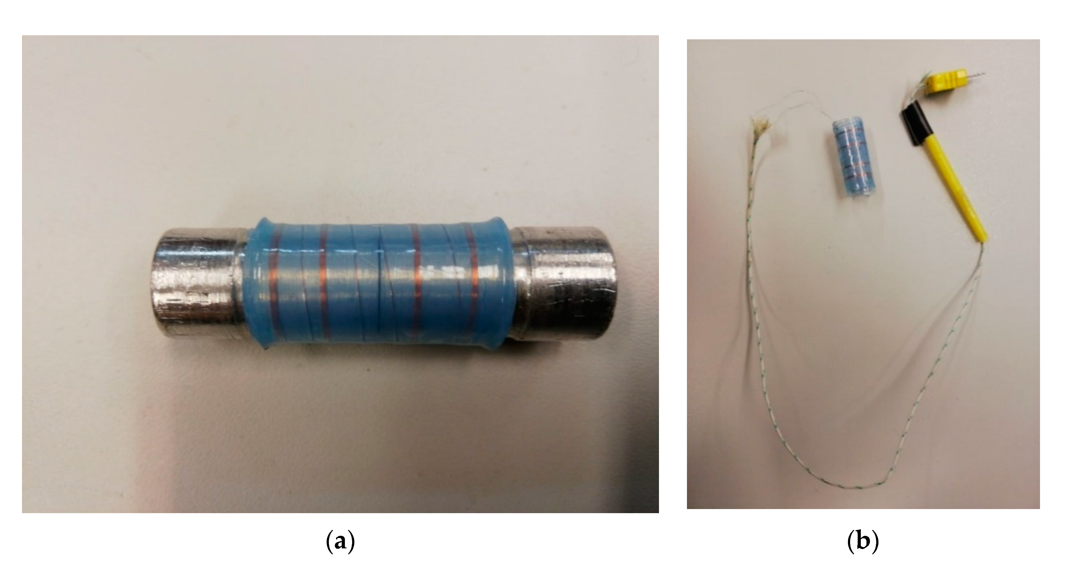
2.4.2. Sample Preparation of IOFEF Joint

The injection molding technique [22] is normally used for the manufacturing of EF joints for water and gas industry. However, at a prototype stage, in order to validate the simulation results shown in Figure 7b and Figure 8b, an in-house IOFEF joint was fabricated. For this purpose, an aluminum mold was used which had an outer diameter of 14.06 mm. A single thin layer of 100 μm LDPE was wound on an aluminum mold to facilitate the winding of 0.1 mm diameter enameled copper joule heating wire. To start the winding, one end of the copper wire was heat buried inside the first 100 µm LDPE layer. By holding one end of the copper wire inside the LDPE layer, the joule heating wire was wound on the mold in a 6 + 1 + 6 + 1 + 1 + 6 + 1 + 6 turn winding pattern. The winding pattern was six turns of a 0.1 mm diameter wire for the first heating zone, followed by one turn to the second heating zone. Then six turns to the second heating zone, with one turn to the middle of the joint being wound. After winding of the joule heating wire, the other end of the copper wire was also heat buried on that side, so the wire did not become loose. After this, a 200 μm LDPE layer was wound, and both ends of the joule heating wire were taken out of the first 200 µm LDPE layer and soldered together. In this way, a closed current path was created inside the IOFEF joint without any need for connector rings, as were used in the ROFEF joints. After the first layer of 200 µm, a custom built 50 µm K-type thermocouple was inserted at layer Lo200, and three more layers of 200 μm LDPE were wound and sealed at the end with a soldering iron.
The whole IOFEF joint assembly with embedded 50 μm was then heated with a hot air gun. By carefully monitoring the temperature of the aluminum mold and the IOFEF joint assembly with a Fluke Ti9 thermal imager, the assembly was heated up to 130 °C so that a homogeneous and uniform IOFEF joint was produced. The resulting validation sample is shown in Figure 10a,b.

2.4.3. Welding of the IOFEF Joint

For welding and measurement of the welding parameters, the following equipment shown in Table 2 was required.

2.4.4. Validation Procedure

  • Connect the output terminals of the controller board, shown in Figure 3c, to the input power of the inductive welding circuit, as shown in Figure 11a. The blue wire in Figure 11a is the +tive input and the yellow wire is the −tive input of the induction circuit.
  • Connect the diffused thermocouple of the IOFEF joint sample to the input of the Picolog TC-08 thermal data logger and insert the welding sample inside the work coil of the induction circuit.
  • Connect the output terminal of the Keysight current probe N2782B to the Rohde and Schwarz RTM1054 oscilloscope Channel 2.
  • Connect the output terminal of the Testec TT-SI 9110 differential voltage probe to the Rohde and Schwarz RTM1054 oscilloscope Channel 1.
  • Set the trigger of the oscilloscope to Channel 1.
  • Connect N2782B current probe to the specially developed IOFEF joint, which has an open wire connection between the two sides of joule heating coils to facilitate current measurement through the IOFEF joint.
  • Connect the Testec TT-SI 9110 differential voltage probe to the input of the work coil.
  • Connect the PICkit 3 to the UART data pins of the controller board.
  • Connect the provided 38 volts 160 watt-hour battery to the power input terminal of the controller board.
  • Connect the USB connector of the Picolog TC-08 data logger and USB connector of the PICkit3 programmer to a PC or laptop with MPLAB X IDE v5.05 and Picolog 6 software installed and configured.
  • Start MPLAB X IDE and program the DsPIC microcontroller of controller board for the desired duty cycle of 16% at 80 kHz for charging of the capacitor bank, 70% duty cycle at 80 kHz for discharging, and one second welding time.
  • Start the Picolog 6 software and configure it for the correct terminal and thermocouple type. Start temperature logging in Picolog 6.
  • Press SW2 on the controller board and when the capacitor bank is charged to 35 volts, Led D18 will be turned ON, indicating that the controller board is ready for welding.
  • Press SW1, the capacitor bank will be discharged to the induction circuit while the charging MOSFET will be running at the programmed duty cycle of 70%, and the discharge MOSFET will be completely ON.
  • Depending upon the trigger settings, the oscilloscope will trigger and capture the voltages and currents according to the configuration.
  • The Picolog6 will capture the temperature curve at the desired first 200 μm layer in the IOFEF joint.
  • After a programmed welding time of one second, the charge and discharge MOSFETs of the controller board will be turned off.
  • Wait for at least 400 s for the Picolog 6 software to capture the cooling curve due to natural convection at room temperature.
  • Stop the Picolog 6 temperature recording after the 400 s cooling cycle.
  • Save the captured voltages and currents as CSV files with their screenshots.
  • Save Picolog 6 temperature data.

2.5. Pull Strength Test

For comparison of joint strength of the mechanical and IOFEF joints, a pull strength test was performed before the air pressure leakage test. In this way, it was made sure that if any kind of joint damage occurs during the pull test, it may be easily visible in the air pressure leakage test.
A thick copper ring was inserted at each end of the welded sample of the IOFEF joint. One end of the test sample was then connected to the base of the Mecmesin MultiTest 2.5-dV machine and the other end was connected to the hook of the AFG 2500N calibrated strength meter, as shown in Figure 11b.
By controlling the pull function of the machine, the two sides of the IOFEF welded microducts were pulled apart to more than 300 newtons. After the pull strength test, the sample was taken out of the machine to proceed to the air pressure leakage test.

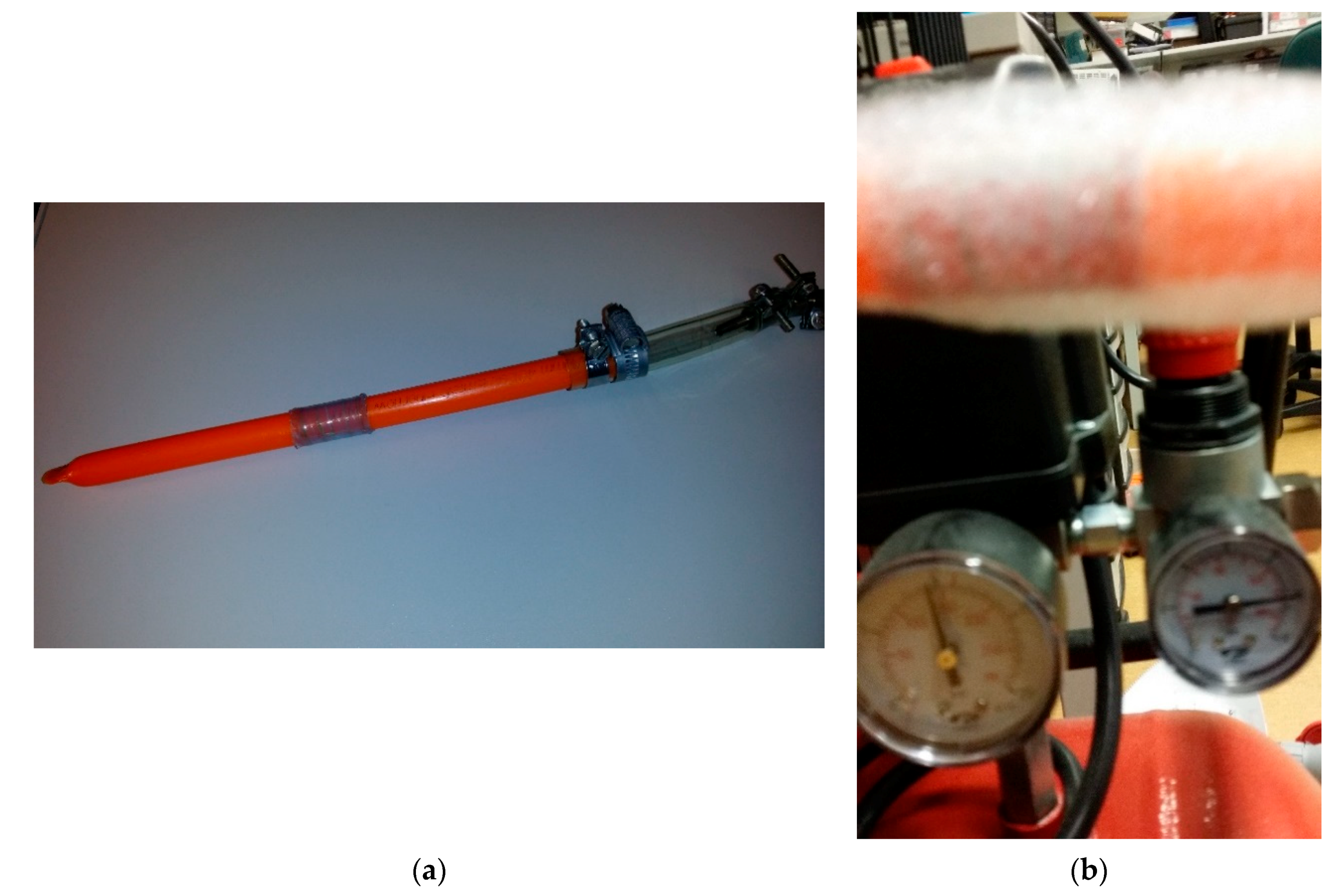
2.6. Air Pressure Leakage Test

After 300 newtons pull strength, the welded IOFEF joint sample was sealed at one end with a hot air gun so that a complete blockage of air was achieved. The other end of the sample was cut with a duct cutting knife to remove the copper ring used for the pull strength test. Due to the unavailability of a 15-bar air compressor, the air pressure leakage test was performed with a 10-bar air compressor. The air pressure nozzle of the air compressor was connected to the sample, as shown in Figure 12a. Despite best efforts, it was impossible to completely stop leakage between the sample and nozzle due to the construction of the hose clamps. The sample was first dipped in a water beaker having a mixture of water and dishwashing liquid and the air pressure of 10 bars was applied. The sample was then taken out of the beaker and the leakage was inspected, as shown in Figure 12b.

3. Results and Discussion

The comparison between the simulated and measured current through the IOFEF joint is shown in Figure 13a. As can be seen from Figure 13a the simulated RMS current through the IOFEF joint was 5.34 A, and the measured RMS current was 5.29 A. It can be easily seen from Figure 13a that the simulated and measured IOFEF joint currents were nearly equal to each other. The difference between the simulated and measured current through the IOFEF joint was because normally ideal components are used for modeling, while real components have certain tolerances and parasitic element values that were difficult to measure with the available instruments. Particularly, the self-resonance of the work coil and IOFEF joint were beyond the 50 MHz range, which could not be measured with the Bode 100 impedance analyzer. This small difference in simulated and measured current inside the IOFEF joint contributed towards measurement tolerances and simulation tolerances. For the development of the IOFEF joint welding system, this current difference is minute and can be ignored easily.
The comparison between the simulated and measured temperature at the first outer 200 µm thick layer is shown in Figure 13b. The measured temperature was 174 °C, and the simulated temperature was 171 °C. Despite all the care in sample preparation and measurement, a difference of 3 °C could be seen between the simulated and measured temperatures. It is important to note that the 50 µm K-type thermocouples were custom built, and with the method defined in Section 2.4.1, and it is still possible to have some uncertainties that cannot be eliminated. During the fabrication of the IOFEF joint sample using a hot air gun and during welding, the K-type 50 µm thermocouple could easily have moved few tens of a micron, and the measurement may differ from the simulation. As can be seen from Figure 13b the cooling curve from 10 s to 250 s has an obvious mismatch between the measured temperature “meas-o200u” and simulated temperature “sim-o200u”. This mismatch was considered to be due to the difference in capacitor discharge rate inside LTspice and the real thermal discharge rate measured with a 50 µm K-type thermocouple. However, this difference in the transient thermal behavior of the developed LTspice model and the real temperature measurement between 10 to 250 s does not influence the peak welding temperature and quality of the weld, and hence was ignored. Thus, it can be concluded that it was still a very good match between the expected and measured peak welding temperature at the first 200 µm thick LDPE outer layer, i.e., Lo200.
In the development of a battery powered inductive welding system, layer Lo200 was selected as a benchmark layer, as it was shown in the work of Akram et al. [3] that reaching a temperature of between 160 °C to 190 °C at Lo200 will guarantee a very good quality ROFEF joint, and which can easily pass the pull strength test of 300 newtons and air pressure leakage test at 10 bars. To verify this result in the IOFEF welding system, the welded IOFEF joint was tested in a non-destructive pull strength test of 300 newtons, and the same IOFEF joint was again tested for air leakage test at 10 bars air pressure, as shown in Figure 11b and Figure 12b, respectively. The welded IOFEF joint successfully passed the pull strength test and air leakage test. The pull strength of the IOFEF joint could be further increased by increasing the wall thickness of the IOFEF joint, and no extra power would be required in such case.
As shown in the work of Akram et al. [3] around 35 joules were available inside the fully charged capacitor bank of 0.056 farads. For welding of ROFEF joint with a 70% duty cycle, 200.16 joules were consumed from the battery and 167.74 joules were dissipated inside the ROFEF joint to reach a temperature of 190 °C at layer Lo200. For welding of the IOFEF joint, 21 joules were consumed from the fully charged capacitor bank, and 306.6 joules were consumed from the battery at a 70% duty cycle. The total dissipated energy inside the IOFEF joint was 158.2 joules to reach a temperature of 174 °C at layer Lo200. When compared to the ROFEF joint, the total energy consumed by the IOFEF joint was 327.6 joules, which is around 64% higher than the energy required for the ROFEF joint. The comparison between the ROFEF joint and IOFEF joint is shown in Table 3.
The complete design of a work coil assembly which can be opened and closed for IOFEF joint insertion was omitted in this study, as it was considered a mechanical design problem. The required connectors were not available off the shelf, and can be custom built. The used work coil will need 34 custom built connectors to complete the current path inside the work coil. The battery used for IOFEF welding was rated at 36 volts 160 watt-hour, but its output voltage was measured to be 38 volts, and therefore 38 volts were used in simulations. A 36 volt 320 watt-hour rated battery of the same weight and size is also available at the same price. By using a higher power battery, i.e., 36 volts 320 watt-hour, it would be possible to power a thicker, i.e., 4.0 mm Litz wire, which would require only nine turns to power the same IOFEF joint. For this purpose, the developed simulation model can be used and the controller board can be programmed to deliver nearly the same power of 158–160 joules to weld an IOFEF joint for a 14.07 mm diameter optical fiber duct. The use of a higher power battery, in turn, would reduce the number of custom built connectors to 18, but would require a higher current input. Therefore, multiple possibilities exist for work coil design and power input methods to further improve the IOFEF welding system.

4. Conclusions

It can be concluded that with a power input of 327.6 joules it was possible to inductively weld a 28 turn 0.1 mm diameter diffused joule heating wire joint on a 14.07 mm diameter optical fiber microduct. The developed inductive optical fiber electrofusion joint has no risk of corrosion for much longer periods of time in very corrosive environments, i.e., installation through drain pipes or sewage lines. This makes it possible to reblow a new optical fiber cable inside an already occupied microduct. Moreover, inductive optical fiber electrofusion joints are more suitable for reheating or de-welding, which is under investigation. The inductive optical fiber electrofusion joints are easy to manufacture due to the absence of connector rings, but they require around 64% more energy input per weld compared to resistive optical fiber electrofusion joints that have connector rings. The developed inductive optical fiber microduct joint can successfully replace non-metallic or so-called “gas connectors”, which have no metal part, for long-lasting protection against corrosion in the optical fiber industry. However, these non-metal or gas connectors are rated at a very low air pressure leakage protection, i.e., 0.5 bars at max. The developed inductive optical fiber microduct joints have no leakage for more than 10 bars of air pressure, which makes it possible to air blow for a longer distance as compared to traditional gas connectors. These advantages make inductive optical fiber microduct joints the best choice for use in highly corrosive environments, and in applications which require the reblow of new optical fiber cables in already buried microducts.

Author Contributions

Conceptualization, K.B., S.A., and J.S.; methodology, S.A. and K.B.; software, S.A. and K.B.; validation, S.A. and K.B.; formal analysis, S.A. and K.B.; investigation, S.A. and K.B.; resources, K.B. and J.S.; data curation, S.A. and J.S.; writing—original draft preparation, S.A.; writing—review and editing, J.S.; visualization, S.A.; supervision, K.B. and J.S.; project administration, J.S.; funding acquisition, K.B. and J.S. All authors have read and agreed to the published version of the manuscript.

Funding

This research work is part of the project FIBER, funded through the European Regional Development Fund.

Conflicts of Interest

The authors declare no conflict of interest.

References

  1. Griffioen, W. Understanding of Cable in Duct Installation: Do’s and Don´ts. In Proceedings of the 60th IWCS Conference, Charlotte, NC, USA, 7–9 November 2011; pp. 198–205. [Google Scholar]
  2. Burdin, V.A.; Nikulina, T.G.; Alekhin, I.N.; Gavryushin, S.A. Researches of optical cable stability in the microduct to effect of freezing water. In Proceedings of the Optical Technologies for Telecommunications 2010; Andreev, V.A., Burdin, V.A., Sultanov, A.H., Morozov, O.G., Eds.; SPIE: Washington, DC, USA, 2010; Volume 7992, p. 79920K. [Google Scholar] [CrossRef]
  3. Akram, S.; Siden, J.; Duan, J.; Alam, M.F.; Bertilsson, K. Design and Development of a Battery Powered Electrofusion Welding System for Optical Fiber Microducts. IEEE Access 2020, 8, 173024–173043. [Google Scholar] [CrossRef]
  4. Griffioen, W. The installation of conventional fiber-optic cables in conduits using the viscous flow of air. J. Lightwave Technol. 1989, 7, 297–302. [Google Scholar] [CrossRef]
  5. Majid, F.; Elghorba, M. HDPE pipes failure analysis and damage modeling. Eng. Fail. Anal. 2017, 71, 157–165. [Google Scholar] [CrossRef]
  6. Bowman, J. A review of the electrofusion joining process for polyethylene pipe systems. Polym. Eng. Sci. 1997, 37, 674–691. [Google Scholar] [CrossRef]
  7. Fujikake, M.; Fukumura, M.; Kitao, K. Analysis of the electrofusion joining process in polyethylene gas piping systems. Comput. Struct. 1997, 64, 939–948. [Google Scholar] [CrossRef]
  8. Shi, J.; Zheng, J.; Guo, W.; Xu, P.; Qin, Y.; Zuo, S. A Model for Predicting Temperature of Electrofusion Joints for Polyethylene Pipes. J. Press. Vessel Technol. 2009, 131, 303–313. [Google Scholar] [CrossRef]
  9. Shi, J.; Zheng, J.; Guo, W.; Qin, Y. Defects classification and failure modes of electrofusion joint for connecting polyethylene pipes. J. Appl. Polym. Sci. 2012, 124, 4070–4080. [Google Scholar] [CrossRef]
  10. Allen, N.S.; Palmer, S.J.; Marshall, G.P.; Luc-Gardette, J. Environmental oxidation processes in yellow gas pipe: Implications for electrowelding. Polym. Degrad. Stab. 1997, 56, 265–274. [Google Scholar] [CrossRef]
  11. Troughton, M.J. Handbook of Plastics Joining: A Practical Guide, 2nd ed.; PDL Handbook Series; William Andrew: Norwich, NY, USA; TWI/The Welding Institute: Cambridge, UK, 2008; p. 110. ISBN 978-0-8155-1581-4. [Google Scholar]
  12. Akram, S.; Bertilsson, K.; Siden, J. LTspice Electro-Thermal Model of Joule Heating in High Density Polyethylene Optical Fiber Microducts. Electronics 2019, 8, 1453. [Google Scholar] [CrossRef] [Green Version]
  13. Roslan, M.; Azis, N.; Kadir, M.; Jasni, J.; Ibrahim, Z.; Ahmad, A. A Simplified Top-Oil Temperature Model for Transformers Based on the Pathway of Energy Transfer Concept and the Thermal-Electrical Analogy. Energies 2017, 10, 1843. [Google Scholar] [CrossRef] [Green Version]
  14. Moumouni, Y.; Jacob Baker, R. Concise thermal to electrical parameters extraction of thermoelectric generator for spice modeling. In Proceedings of the 2015 IEEE 58th International Midwest Symposium on Circuits and Systems (MWSCAS), Fort Collins, CO, USA, 2–5 August 2015; Volume 2015-Sept., pp. 1–4. [Google Scholar]
  15. Wang, Z.; Qiao, W. A Physics-Based Improved Cauer-Type Thermal Equivalent Circuit for IGBT Modules. IEEE Trans. Power Electron. 2016, 31, 6781–6786. [Google Scholar] [CrossRef]
  16. Zhao, R.; Badstieber, C.; Bernaerts, M.; Erbs, F.; Garnier, V.; Goncalves, V.; Harrop, M.; Knott, M.; Laferriere, J.; Martin, T.; et al. Deployment & Operations Committee. In FTTH Handbook, 8th ed.; Connolly Bull, E., Ed.; Fiber to the Home Council Europe: Brussels, Belgium, 2018; p. 113. [Google Scholar]
  17. Sutehall, R.; Davies, M.; Spicer, L.; Gill, P.; Piras, F. Development of an Optical Fibre Cable Overblowing System. In Proceedings of the 67th International Cable and Connectivity Symposium (IWCS 2018), Providence, RI, USA, 14–17 October 2018; pp. 686–693. [Google Scholar]
  18. Reshma, K.K.; Binoy, B.B. ZVS high—Frequency series resonant inverter for induction heating applications. In Proceedings of the 2015 International Conference on Power, Instrumentation, Control and Computing (PICC), Thrissur, India, 9–11 December 2015; IEEE: Thrissur, India, 2015; pp. 1–5. [Google Scholar]
  19. Noda, Y.; Ogiwara, H.; Itoi, M.; Nakaoka, M. A single-stage type highly efficient ZVS-SEPP high frequency inverter for induction heating applications. In Proceedings of the 2014 16th International Power Electronics and Motion Control Conference and Exposition, Antalya, Turkey, 21–24 September 2014; IEEE: Antalya, Turkey, 2014; pp. 53–58. [Google Scholar]
  20. Komori, Y.; Yamanaka, K.; Hojo, M. Fabrication and Verification of Power Supply for Induction Heating. In Proceedings of the 2018 21st International Conference on Electrical Machines and Systems (ICEMS), Jeju, Korea, 7–10 October 2018; IEEE: Jeju, Korea, 2018; pp. 2268–2273. [Google Scholar]
  21. Cengel, Y.A. Heat Transfer A Practical Approach, 2nd ed.; McGraw-Hill: New York, NY, USA, 2003; p. 214. [Google Scholar]
  22. Chebbo, Z.; Vincent, M.; Boujlal, A.; Gueugnaut, D.; Tillier, Y. Numerical and experimental study of the electrofusion welding process of polyethylene pipes. Polym. Eng. Sci. 2015, 55, 123–131. [Google Scholar] [CrossRef] [Green Version]
Figure 1. Mechanical joint types: (a) With and without lock; (b) With IP68 water protection jacket; (c) Straight duct for multiduct installation; (d) Outer plastic lock ring and inner metallic lock ring.
Electronics 10 00743 g001
Figure 2. Sketch of an electrofusion joint used in water, gas, sewage, chemical, and nuclear plants.
Electronics 10 00743 g002
Figure 3. Previous work by Akram et al. [3]: (a) developed the LTspice electrothermal model; (b) fabricated resistive type optical fiber electrofusion joint (ROFEF) with an aluminum mold; (c) controller board with PWM and capacitor bank of 0.056 farads.
Electronics 10 00743 g003
Figure 4. Sketch of inductive-type optical fiber electrofusion (IOFEF) joint with layer distribution used for thermal parameter extraction.
Electronics 10 00743 g004
Figure 5. Work coil for power transfer to IOFEF joints.
Electronics 10 00743 g005
Figure 6. Schematic of the zero voltage switching (ZVS) induction welding circuit used for power transfer to IOFEF joints.
Electronics 10 00743 g006
Figure 7. Electrothermal non-contact welding model: (a) LTspice simulation model for IOFEF welding; (b) Simulation result of one second current through IOFEF joint; (c) Simulation result of 20 s temperature at Lo200.
Electronics 10 00743 g007aElectronics 10 00743 g007b
Figure 8. (a) Equivalent electrothermal model for faster LTspice simulation; (b) Comparison of the original and equivalent simulation models.
Electronics 10 00743 g008
Figure 9. K-type 50 μm thermocouple: (a) 50 μm Chromel and Alumel wires; (b) Bead size of fabricated 50 μm K-type thermocouple.
Electronics 10 00743 g009
Figure 10. IOFEF joint sample preparation: (a) Without thermocouple on aluminum mold; (b) Complete IOFEF joint sample with 50 μm K-type thermocouple.
Electronics 10 00743 g010
Figure 11. IOFEF joint welding sample: (a) Measurements during welding; (b) Pull strength test after welding.
Electronics 10 00743 g011
Figure 12. IOFEF joint welding sample: (a) Sample for air pressure test; (b) Air pressure test after welding.
Electronics 10 00743 g012
Figure 13. (a) Measured current through the IOFEF joint; (b) Measured thermal response of 300 s at Lo200.
Electronics 10 00743 g013
Table 1. Parameters of the work coil and inductor for the LTspice model.
InductorInductanceSeries ResistanceParallel ResistanceParallel Capacitance
L1 and L20.72 µH5 mΩ1 kΩ0.2 pF
L3336 µH49 mΩ9.26 kΩ28 pF
Table 2. Equipment and software required for the validation experiment.
EquipmentModel/Status
IOFEF joint sampleWith 50 μm K-type thermocouple
Controller boardAs shown in Figure 3c.
Differential Current probeAgilent N2782B with N2779A PSU
Differential Voltage ProbeTestec TT-SI 9110
Battery38 volts 160 watt-hour Li-Ion Fully charged
OscilloscopeRohde and Schwarz RTM1054
Thermal data loggerPicolog TC-08
ProgrammerPICkit 3
PC or LaptopInstalled MPLAB X IDE v5.05 and Picolog 6 software
Table 3. Comparison of ROFEF and IOFEF joint.
PropertyROFEF JointIOFEF Joint
Joint length34 mm30 mm
Weight1.5 g1.2 g
Power consumed at 70% duty cycle200.16 joules327.6 joules
Temperature at layer Lo200190 °C174 °C
Pull strength300 newtons300 newtons
Air pressure10 bars10 bars
Publisher’s Note: MDPI stays neutral with regard to jurisdictional claims in published maps and institutional affiliations.

