J-CO: A Platform-Independent Framework for Managing Geo-Referenced JSON Data Sets

Abstract

Internet technology and mobile technology have enabled producing and diffusing massive data sets concerning almost every aspect of day-by-day life. Remarkable examples are social media and apps for volunteered information production, as well as Open Data portals on which public administrations publish authoritative and (often) geo-referenced data sets. In this context, JSON has become the most popular standard for representing and exchanging possibly geo-referenced data sets over the Internet.Analysts, wishing to manage, integrate and cross-analyze such data sets, need a framework that allows them to access possibly remote storage systems for JSON data sets, to retrieve and query data sets by means of a unique query language (independent of the specific storage technology), by exploiting possibly-remote computational resources (such as cloud servers), comfortably working on their PC in their office, more or less unaware of real location of resources. In this paper, we present the current state of the J-CO Framework, a platform-independent and analyst-oriented software framework to manipulate and cross-analyze possibly geo-tagged JSON data sets. The paper presents the general approach behind the J-CO Framework, by illustrating the query language by means of a simple, yet non-trivial, example of geographical cross-analysis. The paper also presents the novel features introduced by the re-engineered version of the execution engine and the most recent components, i.e., the storage service for large single JSON documents and the user interface that allows analysts to comfortably share data sets and computational resources with other analysts possibly working in different places of the Earth globe. Finally, the paper reports the results of an experimental campaign, which show that the execution engine actually performs in a more than satisfactory way, proving that our framework can be actually used by analysts to process JSON data sets.

1. Introduction

Internet technology and mobile technology have enabled the massive production of information concerning more or less any aspect of day-by-day life. In fact, social media, mobile devices and apps for volunteered information production have contributed to gather huge volumes of possibly geo-referenced data sets. Nevertheless, public administrations are producing a very large number of publicly available data sets concerning the administrated territory, known as Open Data, on dedicated portals. Often, Open Data are geo-referenced data sets describing authoritative information about territories, such as boundaries of municipalities, roads, public transportation lines, and so on and so forth.

The most popular standard for distributing these data sets is JSON (acronym for JavaScript Object Notation) [1]: its success is due to the flexibility it provides, because it is a simple serialized representation of main-memory objects managed by object-oriented programming languages; with respect to XML (eXtensible Mark-up Language) [2], it is simpler and faster to manage JSON data sets than XML documents. The GeoJSON format [3,4] is a remarkablGIS (Geographical Information Systems), which is based on JSON.

Currently, many technologies are available or are under development to store and manage large JSON data sets, including NoSQL (that stands for Not only SQL) database systems [5], which are becoming quite popular, such as MongoDB [6]. However, as usual, one single technology is not enough to fully deal with every kind of data set; furthermore, we cannot think that a unique and central storage system could store all data sets to manage, especially when complex cross-analysis tasks must be performed by analysts. We are also envisioning virtual JSON stores, i.e., abstractions of JSON stores obtained by aggregating links of JSON data sets of interest available on the Internet (for example, published by Open Data portals); we figure out that such virtual JSON stores could provide only a read-only access method.

Unfortunately, when different storage technologies are involved, analysts wishing to integrate data sets encounter objective obstacles, such as proprietary or missing query languages, different computational capabilities, restricted or impossible access to JSON stores in writing mode, and different user interfaces. In other words, we observed the lack of a unifying framework and of a unifying query language suitable for people without (or with basic) programming skills. Due to the distribution of data storage systems on different servers, possibly located far away each other, as well as to the availability of the necessary computational resources on remote servers (like cloud servers), analysts who share data sets with other investigation teams located in various parts of the Earth globe should exploit those computational resources remotely, comfortably working in their office. This perspective further complicates the panorama.

These considerations became clear in our mind while participating to the Urban Nexus project [7], a joint effort of geographers and computer scientists to develop models and tools for studying mobility on the basis of Big Data, Open Data and Social Media. The project involved three European research institutions, i.e., University of Bergamo (Italy), Ecole Polytechnique Fédérale de Lausanne (EPFL) (Switzerland) and Angila Ruskin University of Cambridge (UK). So, in 2017 we conceived a new framework, named J-CO (that stands for JSON COllections). The original goal of the framework was to provide a high-level query language able to natively manipulate collections of JSON documents possibly exploiting their geo-tagging, so as to allow geographers to perform complex analysis tasks.

Although started as part of the Urban Nexus project, now it is an autonomous project. Currently, the goal of the framework is twofold: it has to provide a platform-independent view of several (possibly remote) data storage services, storing possibly geo-tagged JSON data sets; it has to provide a query language, named J-CO-QL, for manipulating sets of JSON documents, by natively supporting spatial representations and operations.

This paper presents an extensive review of the organization of the framework, by discussing how the integration of the concept of platform independence (with respect to storage technology) and of the loosely-coupled approach has led us to devise a powerful framework for providing data analysts with a tool for cross-analyzing heterogeneous JSON data sets. With respect to our previous publications [8,9,10] the main contribution of the paper is to provide an organic and comprehensive description of the current state of the framework, which, after re-engineering the J-CO-QL Engine (the execution engine of J-CO-QL) and adding novel components, has assumed the nature of a loosely-coupled and platform-independent framework for manipulating and transforming (possibly geo-tagged) JSON data sets. Specifically, the novel components are the storage service for large single JSON documents (named J-CO-DS) and the user interface (named J-CO-UI), which allows analysts to comfortably share data sets and computational resources with other analysts possibly working in different places of the Earth globe. The J-CO Framework is not a database system, but a tool that provides a platform-independent query language and processing capabilities to retrieve data sets from various JSON stores (not necessarily DBMSs, i.e., DataBase Management Systems), cross-analyze them and possibly store results into its own storage service J-CO-DS (in place of other JSON stores that could provide only a read-only access mode). As a final contribution, for the first time the paper analyzes performance of the execution engine; the results show that it performs quickly with compact data sets and scales properly when the size of data sets increases. Consequently, we can claim that the J-CO Framework is ready to be actually used by analysts.

The paper is organized as follows. Section 2 presents the background of our project and related work. Section 3 introduces the J-CO Framework, specifically focusing on the novel components and on the main features of the re-engineered J-CO-QL Engine. Section 4 introduces the J-CO-QL language, by means of a simple, yet non-trivial, cross-analysis example, by means of which key instructions of the language are presented. Section 5 presents the latest component added to the framework, i.e., the user interface named J-CO-UI. Section 6 reports the experimental campaign and discusses the results. Finally, Section 7 draws the conclusions.

2. Background and Related Work

We now illustrate the background of our research. First, we present the motivations of our proposal. Then, we present related research work.

2.1. Background of the Proposal

The first step towards the idea of a loosely-coupled and platform-independent framework for managing JSON data sets was suggested after the work on the FollowMe project [11,12]: in that project, we had the idea of exploiting social media to trace movements of users. We chose the name “FollowMe” because we traced travelers that posted geo-located messages on Twitter; travelers were detected in a pool of 30 airports connected with the airport of Bergamo (northern Italy), since we wanted to study the relevance of this airport in relation to EXPO 2015, held in Milan (only 40 km separate Milan from Bergamo). Then [13], we integrated the FollowMe project within a framework for analyzing trips of Twitter users; in particular (see [14]), we developed a clustering technique for identifying common paths followed by travelers during their trips. In this preliminary work, trips of Twitter users were represented as JSON documents; we had to analyze them on the basis of a multi-paradigmatic approach (see the Urban Nexus project [7]). While facing this analysis task, we experienced the limitations of current SQL and NoSQL technology when managing heterogeneous geo-located data in the form of JSON documents.

As mentioned above, we had the idea of the J-CO Framework while working in the Urban Nexus project [7]. The goal of this project was to study how city users (inhabitants and commuters) live the city, by means of Big Data, Open Data and any kind of Web source. The project integrated authoritative data sets, statistical data sets and data from social media. In fact, we argued that novel information sources and Big Data (intended as variety of data sets and sources, on the basis of the Seven V’s model [15]) can be beneficial to foster geographical studies about how people live territories. In this project, we realized that data come from many sources as JSON or GeoJSON [3] data sets; we also realized that geographers and analysts ask for high-level tools to work on data sets. These considerations inspired the research work on the J-CO Framework.

2.2. Related Work (on NoSQL Databases and on Query Languages for JSON Documents)

The advent of XML in the late 1990s as the standard format for representing semi-structured documents, for exchanging them through the Internet, gave researchers the idea to investigate the development of database technology for storing XML documents. A large number of proposals came out from this research topic: the reader can refer to [16,17,18] for some surveys. The common feature of all these proposals is that they are XML-native databases, i.e., databases that natively store XML documents (independently of the underlying technology); thus, they constitute an early investigation towards NoSQL databases, because they abandoned the relational data model. XML-native databases had impact on data mining research as well: in fact, the ability of XML to represent both raw data and mined patterns opened the perspective of using XML and XML-native databases to store both data and mined patterns within a unifying representation framework [19,20]. However, some practical obstacles, concerned with the complexity of managing XML documents and their excessive verbosity, have limited XML to become “the representation format” for the Internet. In contrast, JSON has been favored in this sense.

JSON has become the most popular standard for exchanging data sets between different layers of the same web information system and, very often, between different information systems; furthermore, many web services and social-media APIs (Application Programming Interfaces) adopt JSON to exchange data sets. Consequently, the area of NoSQL databases started developing NoSQL DBMSs to natively store JSON data sets. An interesting survey on NoSQL databases is [5], where several systems are cataloged and classified.

One common feature of most NoSQL databases is that they abandon the ACID (Atomicity, Consistency, Isolation, Durability) properties of transactions (as provided by relational DBMSs) in favor of the Base (Basically Available, Soft state, Eventual consistency) model [21,22] to deal with concurrency. In particular, since JSON data are generically called “documents” [23], a DBMS able to natively store JSON documents falls into the category of document databases. One of the most famous representatives is MongoDB [6]. Readers interested in NoSQL DBMSs evaluation can refer to [5,22].

Obviously, the diffusion of JSON and of JSON-native DBMS technology asks for suitable and high-level query languages. Before defining our query language named J-CO-QL [9,10] (see Section 4 for a synthetic introduction), we studied previous proposals. Hereafter, we present the most relevant languages. We compare their features with those that characterize J-CO-QL;

Table 1. Comparison of query languages for JSON data.

Query Language	J-CO-QL	Jaql	SQL++	JSONiq	MongoDB
1. Adaptability to heterogeneity	YES	NO	NO	NO	NO
2. Spatial operations	YES	NO	NO	NO	YES
3. Platform independence	YES	NO	YES	YES	NO
4. Re-use of intermediate results	YES	NO	NO	NO	NO
5. Orientation to Analysts	YES	NO	YES	NO	NO
6. Orientation to Programmers	NO	YES	NO	YES	YES

synthetically reports the results of the comparison; the table considers only those languages that operate on JSON documents; rows report the features we considered. Specifically, they are introduced below.

• Adaptability to heterogeneity. This feature refers to the ability of the language to manipulate heterogeneous documents with one single instruction. In fact, usually query operators have sets of documents as operands; sets of documents may contain heterogeneous documents, i.e., documents having (possibly many) different structures from each other; if the operators are able to work on documents with totally different structure with one single instruction, i.e., processing them all together, the feature called Adaptability to heterogeneity is met. In contrast, if operators deal with one single structure at a time, this feature is not met.
• Spatial operations. This feature refers to the capability of performing spatial operations on geo-tagged documents.
• Platform independence. This feature refers to the fact that the query language is independent of a specific platform, typically JSON document stores.
• Re-use of intermediate results. When complex transformations are performed, intermediate results could be precious for next processing steps. With this feature, we refer to the capability of the query language to explicitly handle and re-use intermediate results, to avoid re computations as well as to avoid storing intermediate results temporarily within JSON databases.
• Orientation to Analysts. This feature refers to the fact that operators of the query language are oriented to analysts, without specific procedural programming skills.
• Orientation to Programmers. This feature refers to the fact that operators of the query language are oriented to computer programmers, having strong computer programming skills.

After this premise, we can start presenting various languages for querying JSON data sets.

Jaql was proposed in [21] to help Hadoop (the popular Map-Reduce framework, see [24,25]) programmers develop complex transformations, when writing Map-Reduce programs on Big Data. It is designed to be flexible and independent of the physical representation of data. Furthermore, since it is thought for the Map-Reduce paradigm, where complex computations are modeled as sequences of Map-Reduce phases, Jaql strongly relies on the concept of “pipe”. Considering the features reported in Table 1, Jaql does not support heterogeneity of documents, does not provide spatial operations, is not platform independent, does not provide re-usability of intermediate results and is oriented to programmers.

The language that we repute the best proposal before J-CO-QL is SQL++ [26]. Its semi-structured data model is designed as an extension of both JSON and the relational data model; consequently, the language is derived from the classical SELECT statement by adding a limited number of language extensions. In this sense, [27] reports the case of N1QL for Analytics, an interesting implementation of SQL++ for the Couchbase Server. Considering the features reported in Table 1, SQL++ is not specifically designed to work with heterogeneous documents in an explicit way, as well as spatial operations are not considered at all. It is platform independent, but it does not provide re-usability of intermediate results and it is oriented to analysts (because it derives from SQL).

JSONiq [28] is a query language for JSON documents derived from XQuery [29]. The functional style of the language, the semantics of comparisons in case of data heterogeneity and the declarative snapshot-based updates are taken from XQuery, while other specific features are not suitable for querying JSON documents, such as management of mixed content, because they are peculiar of XML. However, like XQuery, it can be hardly used by inexperienced users. Considering the features reported in Table 1, JSONiq is not able to work on heterogeneous documents and does not provide spatial operations; it is platform independent, but it does not provide re-usability of intermediate results and it is not oriented to analysts, while it is oriented to programmers.

The query language provided by MongoDB [5,30], probably the most popular JSON document DBMS, is certainly considered the reference language (URL: https://docs.mongodb.com/manual/, accessed on 3 March 2021). If we consider the features reported in Table 1, it is not designed to manipulate totally heterogeneous documents. It provides spatial operations, but they can be performed only on documents that are materialized in the database (because they must be previously indexed by means of spatial indexes); spatial operations cannot be performed on temporary data. It is not platform independent, because it is specific of MongoDB; re-usability of intermediate results is not natively supported, because they must be saved into the database. The syntax, which is based on object-oriented programming, makes it not specifically oriented to analysts; however, complex transformations can be performed only by writing JavaScript functions within the query, thus this makes the language definitely oriented to programmers.

Other approaches to manipulate heterogeneous big data recognize the importance of a declarative query language [31,32], although they do not work on JSON data sets. The advantage is to simplify coding of complex transformations, in particular in the context of Map-Reduce programming. An interesting example is Spark SQL [33], introduced within the Apache Spark framework, one of the two most-popular frameworks supporting the Map-Reduce paradigm for processing Big Data. It is designed to allow for specifying complex manipulations of data sets without using Map-Reduce primitives (the framework transforms Spark SQL queries into low-level Map-Reduce primitives). However, Spark SQL still does not consider at all spatial operations.

A proposal concerned with spatial operations is GeoSPARQL [34]. It is a Geographic Query Language for RDF data, proposed as a standard by the OGC (Open Geospatial Consortium—URL: https://www.ogc.org/, accessed on 3 March 2021), for querying geospatial data on the Semantic Web. GeoSPARQL is designed to accommodate systems based on qualitative spatial reasoning and systems based on quantitative spatial computation, to ease data analysis. In contrast, it is not designed to work with large JSON data sets, while our framework (and its query language) is oriented to provide data analysts with a tool for managing data about real entities, described by large sets of JSON documents and/or large GeoJSON documents.

The overall J-CO Framework (and the J-CO-QL query language, in particular) relies on our previous research work on collections of complex spatial data [35,36]. In those works, we proposed a database model capable to deal with heterogeneous collections of possibly nested spatial objects; the proposal encompassed an algebra to query complex spatial data, derived from classical relational algebra. In J-CO we follow a different approach: we have not defined a database model, because J-CO relies on JSON data sets. Furthermore, J-CO-QL abandons the classical syntax of relational algebra, in favor of a more flexible syntax, suitable to specify complex transformation processes in a more intuitive and flexible way; in fact, we applied the experience we made in [37], where we defined a language for manipulating clusters of web search results performed through a mobile device.

The J-CO Framework is specifically designed to be loosely-coupled with underlying JSON document stores: it seamlessly accesses any kind of JSON document stores (provided that a connector is available) and provides its own computational capabilities; consequently, J-CO-QL is platform independent (feature 3 in Table 1). This is why we say that it is a “multi-store framework”. In effect, when we defined the approach, we had the concept of PolyStore DBMS in mind; it denotes database management systems that deal with several DBMSs at the same time, each of them possibly providing a different logical model, such as relational, graph, JSON, pure-text, images and videos. It appears that BigDAWG [38] is the first polystore system in the literature; nevertheless, it is not an isolated case and the work on polystores is going on. For example, [39] reports about Polystore++, a polystore system for analytic applications. However, the definition of polystore systems requires the development of techniques for building query plans (as in [40]), as well as to define extensions of the classical relational algebra (as in [41]).

These previous workson polystores clearly adopted a pure database approach, in which it is assumed that the DBMSs integrated within the polystore provide their own and fully exploitable query languages. However, an interesting sentence from [41] says: “Polystores seek to provide a mechanism to allow applications to transparently achieve the benefits of diverse databases while insulating applications from the details of these databases”. The J-CO Framework is not a polystore, since it relies on a unique data model and does not push computation to DBMSs, in order to be platform independent; however, it certainly has been designed in order to make applications insulated from the specific JSON document store technology.

The loosely-coupled design of the J-CO Framework, motivated by the fact that JSON document stores could not provide the necessary processing capabilities or permissions to execute queries, could appear a strange decision to database experts. Currently, the J-CO-QL Engine executes queries only in main memory. However, the world of database systems is more and more getting populated by solutions that manage large data sets in main memory. A field in which this approach could appear paradoxical is Business Intelligence. However, there exist systems (see [42]) that perform Business Intelligence tasks on large volumes of data to aggregate in main memory. The Qlik suite [43,44] is a quite famous suite for Business Intelligence that operates in main memory: it first collects data from data sources into main memory, then it performs aggregations requested by users.

3. A Framework for Manipulating Geo-Referenced Data

In this section, we introduce the J-CO Framework.

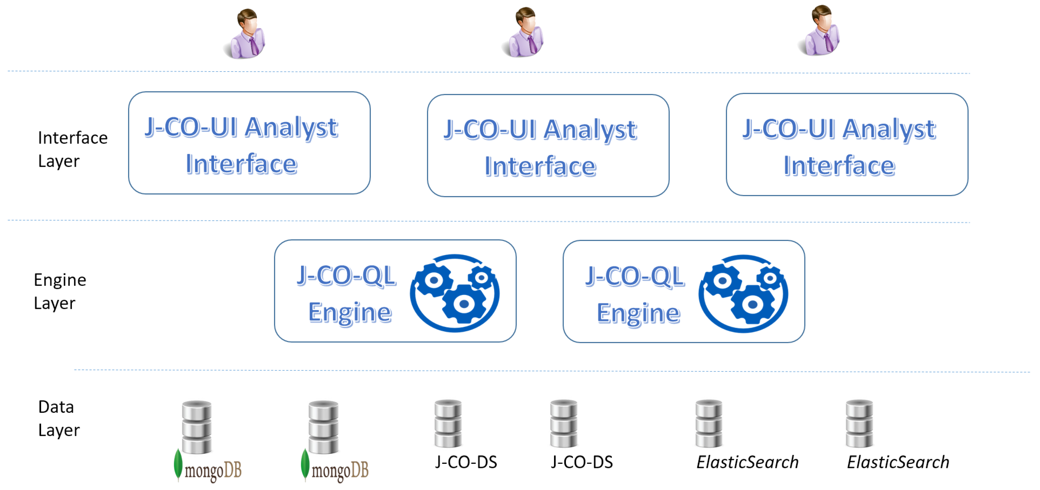
3.1. Organization of the Framework

The framework we conceived for integrating and transforming geo-referenced JSON data is named J-CO (acronym for JSON COllections) and comprehends several components.

• One or more NoSQL storage systems, powered by MongoDB, ElasticSearch [45] and, in the future, other similar systems (for example, AWS Amazon DB, https://aws.amazon.com/documentdb/, accessed on 3 March 2021).
• J-CO-DS is a simplified storage system for sets of JSON documents; since it is based on the file-system, it is able to store very large JSON documents that would not be managed by other systems, like MongoDB. It is not a DBMS, since it neither provides a query language nor supports OLTP operations.
• J-CO-QL is the query language around which the entire framework is built. The language allows for specifying complex transformations, possibly based on spatial operations.
• The J-CO-QL Engine executes J-CO-QL queries by retrieving data stored in one or many JSON storage systems.
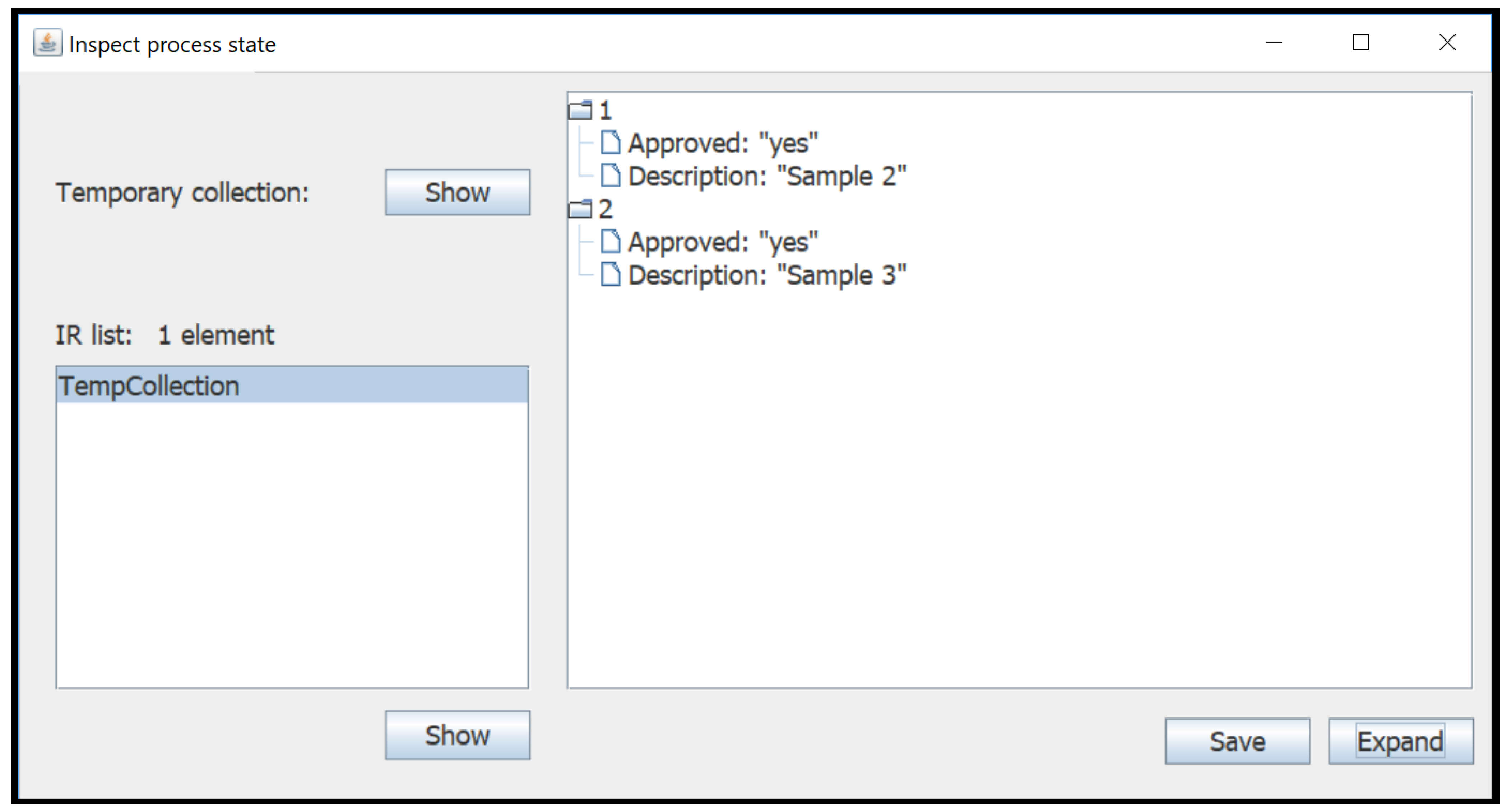
• A User Interface, named J-CO-UI, provides users with a powerful tool to write complex queries step-by-step, by possibly inspecting temporary results of the process.

The overall framework relies on a unique data model.

Definition 1.

Data Model.A “collection” is a set of JSON documents, where documents are heterogeneous, i.e., possibly have their own structure, without limitations. A “database” is a set of collections; neither predefined structures nor schemas for documents in collections are considered.

Hereafter, we give a more detailed description of two key components, specifically J-CO-DS and J-CO-QL Engine. J-CO-QL will be presented in Section 4, while J-CO-UI will be introduced in Section 5.

Now, we present the layer-based view of the framework we reported in Figure 1, which motivates the loosely-coupled design. We considered three layers, i.e., the Data Layer, the Engine Layer and the Interface Layer.

• The Data Layer includes all data stores, managed by any kind of NoSQL storage system (currently, MongoDB, ElasticSearch and J-CO-DS). Since each single data store can contain a relevant piece of information to integrate, they must be viewed in a seamless way by users: they do not have to take care of the specific storage technology.
• The Engine Layer encompasses one or many instances of the J-CO-QL Engine. Why more than one instance? Because it could be installed on several servers, in order to provide many different users, possibly located in different areas of the Earth globe, with the necessary computational power.
• The Interface Layer encompasses one or more installations of J-CO-UI: in fact, users (typically, analysts) write queries and develop transformation processes through this tool. Since J-CO-UI is a desktop application (see Section 5), its instances are installed on analysts’ PCs.

Consequently, we can say that the loosely-coupled design of the J-CO Framework allows for creating an eco-system of data, computational resources and human resources distributed around the world, working together on the same investigation problem. Each single computational resource (user interfaces, J-CO-QL Engine and JSON storage systems) communicate through the Internet and can be easily added to or removed from the eco-system.

Discussion. Thinking about JSON stores, we do not have to think that they are necessarily DBMSs that work on JSON documents instead of relational data; in fact, people usually think that they provide a query language able to transform data items in a way similar to what SQL does (through the INSERT, UPDATE, DELETE and SELECT statements). The scenario is quite different, for various reasons. First of all, we discuss the topic of query languages.

• Some JSON storage systems provide query languages, in a way similar to traditional DBMSs; however, these languages do not provide operations that are familiar to SQL users, like “joins”. An example is MongoDB, in which to perform queries equivalent to “joins” it is often necessary to write procedural JavaScript code, to overcome the limitations of its query language.
• Other JSON storage systems do not provide any query language or capability to transform stored data. ElasticSearch falls into this category: it is an engine for information retrieval, which receives and provides data in JSON format through its API. However, it is not a DBMS: when a document is received, it is indexed by means of an inverted index, that allows keyword-based searches to retrieve indexed documents. Clearly, it has not to provide a query language as intended for DBMSs, because it is not a DBMS.
• In principle, any Open Data portal could be a read-only JSON store: if we had a tool able to provide a database-like abstraction of Open Data portals, we could consider it as a valid JSON store from which data can be read for further processing. Obviously, we cannot expect any processing functionality (in terms of query language) by such sources.

Another point to consider when thinking about JSON storage systems is whether they provide a concurrency model.

• A strong concurrency model is one of the key success factors of relational DBMSs. Some JSON store systems provide strong concurrency models, like CouchDB [25,46], that, for this reason, has been chosen as the DBMS for HyperLedger Fabric [47], the well-known block-chain platform developed by Linux Foundation.
• Originally, MongoDB provided very limited concurrency control and transaction management. Now, as long as it becomes more and more adopted, new versions enrich support to transactions; consequently, it is becoming a true DBMS for JSON documents.
• Other JSON storage systems do not provide any concurrency control or support to transactions. This is the case, for instance, of ElasticSearch.

3.2. J-CO-DS

We decided to develop this storage service when we encountered some limitations exposed by available NoSQL storage systems, in particular, MongoDB and ElasticSearch.

• MongoDB [6] is a true DBMS for JSON data. Its data model is the same we introduced in Definition 1: a “database” is a set of collections, where a “collection” is a set of JSON documents. Neither predefined structures nor schemas must be defined: a collection can store heterogeneous JSON documents, with no limitations. However, MongoDB is designed to manage very large collections of small documents: it does not accept JSON documents whose internal binary representation (the BSON format) is larger than 16MB. This limitation makes impossible to store large GeoJSON documents within MongoDB databases: in fact, a GeoJSON document is a single document that can be giant; in case of complex geometries, the BSON representation can easily exceed 16 MB. Consequently, MongoDB is actually unable to manage very large documents.
• On the other side, ElasticSearch [45] is a very popular tool for performing information retrieval operations. It is not designed to be a pure DBMS, but since it receives and provides JSON data sets through its API, it can be assimilated to the database view. However, it is not good to store very large GeoJSON documents into ElasticSearch, because it has to index the whole document, including geometries; this would cause a significant waste of time (during indexing) and would negatively affect results provided by ElasticSearch at retrieval time, because coordinates would be considered for text-based retrieval as text fragments, not as numbers denoting geo-tagging. ElasticSearch does not provide any query language, in the sense of database query languages: stored data cannot be manipulated as it is possible to do, e.g., within MongoDB. Obviously, its API allows for uploading, getting and deleting data sets.

So, we argued that a data storage service for large JSON (possibly GeoJSON) documents was missing and we decided to develop J-CO-DS.

J-CO-DS provides the same data model as MongoDB: a database is a set of collections, and a collection can contain any kind of (possibly huge) JSON documents. No query language is provided, because J-CO-DS is not meant to be a DBMS: it is a simple JSON storage system, which does not support OLTP operations at document level. J-CO-DS had to be easily developed and fast in retrieving and storing documents: consequently, we adopted a lightweight approach by design, i.e., collections are managed through the file-system. No extra features are provided, neither indexes nor spatial indexes, because J-CO-DS is designed neither for processing queries not for supporting operational activities. In fact, J-CO-DS is thought to be a simple storage system for collections of JSON documents, able to manage large single documents; it can be used by analysts to organize data sets, without the complexity of a pure DBMS, like MongoDB. Note that this approach is perfectly coherent with the rest of the framework, which is designed to be platform independent as far as storage systems are concerned.

Obviously, a managing interface is provided. Hereafter, we present the components of J-CO-DS.

• J-CO-DS Service is the true storage service that can be contacted through a TCP port, either by J-CO-QL Engine instances or by any other application wishing to exploit its services.
• J-CO-DS Manager is a user interface that allows for interactively managing the data store; it is an application that can be installed on administrator’s PC and provides two execution modes:

  –

  Stand-alone mode: in this execution mode, the application uses a text-based interface, that can be accessed through a classical text-based shell;

  –

  Web-based mode: when launched in this mode, the application provides a web-based interface, by means of an internal web server packaged in the executable file.

  Through the user interface, usual basic management operations can be performed, such as database creation and deletion, collection creation and deletion and upload of JSON documents into collections. J-CO-DS does not support transactions and does not provide explicit locking mechanisms, because they are not necessary; only an implicit locking mechanism on collections, when either a read or a write operation is performed, is provided to serialize access to single collections.

3.3. J-CO-QL Engine

The J-CO-QL Engine is the core software component of the framework, because it executes J-CO-QL queries. Recently, it has been re-engineered, in order to be compliant with the multi-layer view depicted in Figure 1. It mainly operates as a service on a specific TCP port. It actually executes J-CO-QL queries, by connecting to data storage services to get and save data sets (collections of JSON documents). Since its re-engineering, it provides two different operating modes:

• Batch Mode: this mode can be used to execute complex and long queries, previously written by analysts.
• Interactive Mode: this mode can be used to write queries step-by-step, so as to build complex transformation processes, in an interactive manner.

In particular, when operating in Interactive Mode, the service provides the following features:

• Long-Term Query Process: the query process lives for a long time, the process state is not lost while waiting for new instructions;
• Step-by-step Issuing: instructions are provided one at a time; if the instruction generates an error (lexical, syntactic or semantic error) simply the process state does not change;
• State Inspection: the current process state can be inspected;
• Roll-back: the user can roll-back the execution of the process to a previous execution state.

These features are controlled by J-CO-UI (see Section 5).

Platform Independence. One of the main goal of the J-CO Framework is being able to access several data sources, managed by different storage technologies. The reason for developing a novel query language (the J-CO-QL query language, presented in Section 4), is to provide a uniform language that is independent of the specific storage platform. In fact, due to the significant differences that characterize capabilities of query languages provided by data storage systems, as well as the possible absence of query languages and processing capabilities, the J-CO-QL Engine cannot transfer any processing activity to data sources. This is beneficial for the evolution of J-CO-QL, in which we plan to add instructions for complex tasks such as machine learning. The following features are related with platform independence.

• Multiple Connectors. The J-CO-QL Engine is equipped with a specific connector for each single data storage system we have considered so far, i.e., MongoDB, ElasticSearch and J-CO-DS. These connectors provide a uniform interface to the code of the J-CO-QL Engine towards different data storage systems.
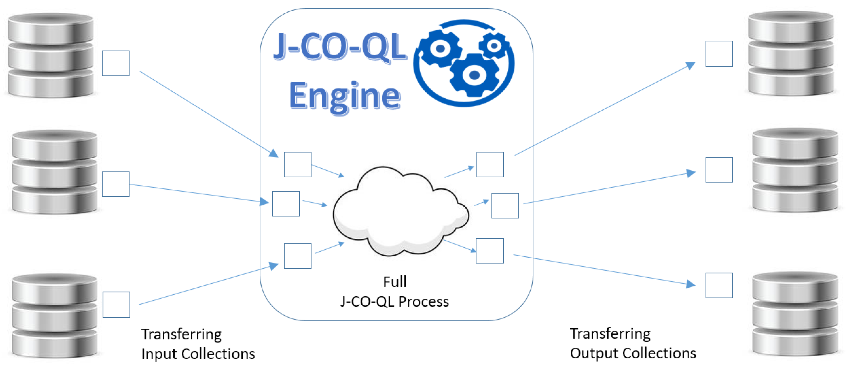
• Retrieving/storing Collections. The J-CO-QL Engine interacts with data storage systems only to retrieve the content of collections and to store new collections. No data processing is asked to data storage systems because input collections are transferred to the J-CO-QL Engine and output collections are transferred to the data storage systems.
• Loosely Coupling. As a result, the J-CO-QL Engine is loosely coupled to data storage systems: all processing activities (i.e., execution of J-CO-QL transformation processes) are performed within the J-CO-QL Engine on the local copy of collections, not on the source databases.

The J-CO-QL Engine is implemented in Java standard edition. This choice further achieves platform independence, in this case as far as the operating system is concerned.

Connectors to storage systems invoke specific APIs provided by them. In particular, the connector to MongoDB has to encode/decode JSON documents to/from the BSON representation.

As far as the management of geometries is concerned, we used the JTS—Java Topology Suite library (URL: https://github.com/locationtech/jts, accessed on 3 March 2021). The library is able to parse GeoJSON geometries represented as GeometryCollection types (see [3]), so as to obtain its own internal representation, suitable to easily perform spatial operations. The library is able to re-generate GeoJSON representations of geometries from its own internal representation.

Currently, all collections are processed only in main memory, without using mass memory. In order to overcome limitations in memory size, as well as to accelerate spatial operations, we plan to introduce hybrid processing methods (main and mass memory) as well as to create (spatial) indexes on the fly.

Discussion. In the application context of our framework, decoupling data source environments from the processing environment is an essential feature. First of all, it is due to the fact that JSON storage systems may not provide any capability to transform data (see the discussion in Section 3.1). As an effect, the J-CO-QL Engine remains independent of actual processing capability (if any) provided by JSON stores (the situation in which no JSON store providing processing capability is connected is possible). Furthermore, the J-CO-QL Engine could implement J-CO-QL operators that cannot be supported by query languages (for example, operators for performing data mining and machine learning activities, that we are planning as future work).

A second, but not less important, reason is concerned with integration of collections coming from different JSON stores: to integrate them, data sets should be moved from one store to another. We do not want users to move data from one store to another (provided that they provide the necessary computational power), because this would limit the flexibility we want to provide analysts with.

In fact, the user can be substantially unaware of where and how a database is managed, because, as depicted in Figure 2, queries and the engine seamlessly operate on collections and integrate them, irrespective of their actual source (Section 4 will highlight this aspect). Thus, we can see the J-CO-QL Engine as a service built on top of other services, specifically JSON stores and NoSQL DBMSs. Thus, it could be a way to somehow “federate” JSON stores. Nevertheless, the J-CO-QL Engine is not a NoSQL DBMS: it simply retrieves data from and store data into databases managed by JSON stores and NoSQL DBMSs, which continue providing their specific functionality: for example, MongoDB serves information systems for operational activities, while ElasticSearch is a document search engine. Thus, the J-CO Framework enables to create a sort of “side federation” of JSON stores currently used for other purposes; this is also a sort of “light federation”, because JSON stores are “federated” only during the time the J-CO-QL Engine is connected to them. At the best of our knowledge, we have found no similar proposals.

4. J-CO-QL: The Query Language of the J-CO Framework

In this section, we introduce J-CO-QL, the query language of the J-CO Framework. First of all, in Section 4.1 we introduce the main features of the language. Then, in Section 4.2 we describe some key instructions of the language by means of an illustrating example.

4.1. J-CO-QL Main Features

J-CO-QL is designed to work with collections of JSON documents (see Definition 1). In a document, fields can be either simple fields (numbers or strings) or complex fields (i.e., nested documents) or vectors (of numbers, strings and documents).

Since J-CO-QL has to natively deal with geo-references, its data model must natively encompass them. However, JSON does not consider geo-references. We decided to rely on the GeoJSON standard [3,4]: fields describing geometries are complex JSON nested documents that can describe points, lines and polygons, as well as collections of them; for this purpose, the GeoJSON standard provides a specific data type named GeometryCollection. In J-CO-QL, geo-references play a special role, since the language provides operators and constructs to handle them. In order to give this special role to geo-references, the J-CO-QL data model considers the special ~geometry field: if present at the root level of a document, this means that the document is geo-referenced (or geo-tagged). The name ~geometry is fully compliant with JSON naming rules, but ~ is rarely used in field names: in our model, it is used to denote a special role of the field. The value of the ~geometry field is based on the GeometryCollection type of the GeoJSON standard.

As an example, consider Listings 1 and 2, which report the excerpts of two collections of documents: Listing 1 reports the excerpt of the collection named Districts, which describes districts of cities in Northern Italy; Listing 2 reports the excerpt of the collection named BikeLanes, which describes bike lanes in Northern Italy. These two collections are inspired by real data sets published on the Open Data portal of Milan (Italy) City Council (URL: https://dati.comune.milano.it/, accessed on 3 March 2021).

The reader can notice that the documents in the BikeLanes collection (Listing 2) have different structures, although they describe the same type of geographical entity, i.e., bike lanes; we will see how J-CO-QL is able to deal with heterogeneous collections.

Furthermore, notice that documents in the Districts collection (Listing 1) are already compliant with the J-CO-QL data model, since they have the root-level ~geometry field. In contrast, documents in the BikeLanes collection (Listing 2) do not have the ~geometry field, but the geometry field (without ~, because they are possibly derived from a GeoJSON document). Consequently, J-CO-QL should provide constructs to align geometries to the J-CO-QL data model.

Listing 1.

Excerpt of collection Districts.

Listing 2.

Excerpt of collection BikeLanes.

As a final remark, notice that coordinates (longitude and latitude) are expressed based on the WGS84 (World Geodetic System) standard, our Coordinate Reference System (CRS); currently no other CRS is supported.

Since the first version of the language [8], J-CO-QL instructions have met the closure property, that is, they get collections and generate collections. Furthermore, the language provides the key features reported hereafter.

• J-CO-QLinstructions are able to deal with documents with different structure with one single instruction. This is the feature named Adaptability to heterogeneity in Table 1.
• J-CO-QL instructions allow for specifying complex transformations oriented to analyze data. This is the feature named Orientation to Analysts in Table 1.
• J-CO-QL instructions directly deal with geo-references (through the ~geometry field) and spatial operations. This is the feature named Spatial operations in Table 1.

J-CO-QL queries (or transformation processes) are sequences of instructions [10,48]. The execution process of queries is based on the concept of state of the query process (or query-process state, in the rest of the paper), which is a pair $s=(tc,IR)$, where $tc$ is a collection named Temporary Collection, while $IR$ is a database named Intermediate Results database.

Each instruction $i_j$ starts from a given query-process state $s_{(j-1)}$ and generates a new query-process state $s_j$. A specific instruction asks the J-CO-QL Engine to store $tc$ (the Temporary Collection) into $IR$ (the Intermediate Results database), so that the collection could be taken as input by a subsequent instruction.

The J-CO-QL Engine executes each query process in isolation: several users can use the same instance of the engine in a concurrent way. Thus, the goal of the $IR$ database, one for each query process, is twofold. First, it temporarily stores intermediate results of the process, so that they do not have to be stored into persistent databases (since they are intermediate results). This is the feature named Re-use of intermediate results in Table 1. Second, it ensures isolation of query process execution as far as intermediate results are concerned.

4.2. Language by Example

In this section, we briefly illustrate J-CO-QL, by showing a short example of cross analysis. Suppose that three data storage systems are involved in the activity: a J-CO-DS server having 10.0.0.11 as (toy) IP address; two MongoDB servers, whose (toy) IP addresses are 10.0.0.12 and 10.0.0.13.

Specifically, we have three databases. The first one is named Boundaries; it is hosted by the J-CO-DS server and stores authoritative data sets about administrative boundaries (since they are usually very large, it could not be possible to store them within MongoDB databases, see Section 3.2); in particular, this database contains the Districts collection (that contains JSON documents describing districts of cities in Northern Italy, such as Milan). Recall that Listing 1 shows an excerpt of this collection.

The second database is named RegionInfo: it is managed by the MongoDB server with IP address 10.0.0.12; it contains collections related with territory. In particular, we have the BikeLanes collection, which contains documents describing the path of bike lanes in Northern Italy. Listing 2 reports an excerpt of this collection (recall that documents have heterogeneous structure).

The third database is managed by the MongoDB server having IP address 10.0.0.13: its name is toShare, because it contains data sets that the analysis team has to share with other teams.

The team of analysts has the following (sample) goal: discovering the bike lanes in the city of Milan that cross at least two districts of the city of Milan. The J-CO-QL query for performing the analysis is reported in Listings 3 and 4. Hereafter, we will explain it, by briefly introducing each single instruction. The reader can exploit Figure 3, which reports the execution trace of the process: the trace starts with the empty query-process state $\left(\right[],\{\left\}\right)$ taken as input by the first GET COLLECTION instruction (line 4 of Listing 3); the query-process state produced by each single instruction is reported (for simplicity, we do not report the actual content of temporary collections, but only an identifier $t_i$, where i is the line that generates the temporary collection $t_i$).

Listing 3.

Sample transformation process written by means of J-CO-QL (part 1).

Listing 4.

Sample transformation process written by means of J-CO-QL (part 2).

This execution model derives from the semantics of relational algebra, where an operator produces a table that is taken as input by the next operator; in relational algebra, the inverted syntax of unary operators (operands are behind the operators) and the infix syntax of binary operators make writing queries somehow unnatural. In J-CO-QL, instructions implicitly start from the query-process state possibly generated by the previous instruction and generate a new query-process state, which contains a possibly modified version of the temporary collection; thus, a query is a kind of “pipe” of instructions, that are written in the same order as they are thought. In fact, J-CO-QL is neither procedural nor imperative: no variables and no instructions to control the execution flow (like cycles) are provided. Instructions specify complex transformations on documents in a declarative way, following the same approach behind the SELECT statement of SQL, which is the reason why SQL is widely used by people without programming skills to query and analyze data.

Let us start describing the first part of the query, reported in Listing 3.

• First of all, it is necessary to specify which databases to connect to. The three USE DB instructions at lines 1–3 do this work. Notice that the ON clauses specify the connection strings necessary to connect to the desired servers. These instructions do not change the query-process state; consequently, both temporary collection and Intermediate Results database $IR$ remain empty; this is why in Figure 3 we start depicting the query process form line 4.
• The GET COLLECTION instruction at line 4 gets the Districts collection from the Boundaries database: the collection becomes the new temporary collection $t_4$ of the query process (as depicted in Figure 3).
• The FILTER instruction at line 5 actually filters documents that describe districts of Milan. It takes the current temporary collection $t_4$ and applies the CASE WHERE clause, which is a document selection condition. In the instruction, the condition relies on the WITH predicate: this predicate is true if the document under selection contains the specified field (or fields, if a list of field names is specified). In the specific case, the condition is true if the document under selection contains the City field within the root-level Properties field and if its value is “Milan”.
  For each document that meets the condition, the GENERATE action inserts a restructured version of the document into the output temporary collection $t_5$, such that the ID field is reported as it is, while a new root-level Name field is derived from the previously nested one (specified by the expression .Name: .Properties.Name). The ~geometry field is kept as it is, as specified by the KEEPING GEOMETRY directive.
  The final DROP OTHERS option specifies that documents that do not meet the selection condition must be discarded and will not appear in the output collection (the language admits an alternative KEEP OTHERS option, which would keep not-selected documents into the output collection). We introduced this option to make J-CO-QL adaptive to heterogeneity (feature 1 of Table 1).
  The output collection becomes the new temporary collection $t_5$. An excerpt is reported in the upper part of Listing 5, where the restructured version of documents shown in Listing 1 is reported.
  In the CASE WHERE clause and in the GENERATE action, fields are referred to by means of a dot notation like .A.B.C, in order to deal with nested documents (the sample dot notation would access the C field nested within a B field, in turn nested within the A field at the root level of the document).
• The temporary collection $t_5$ produced by line 5 contains only districts of Milan. Line 6 saves this temporary collection into the Intermediate Results database $IR$ with name Milan_Districts, for further processing during the same query process; this is the feature Re-use of intermediate results reported in Table 1. In Figure 3, notice how the $IR$ database is no longer empty in the query-process state produced by line 6.
• Lines 7 to 9 basically perform, on bike lanes, the same task performed by lines 4 to 6. Specifically, line 7 gets the BikeLanes collection from the RegionInfo database; this collection becomes the new temporary collection $t_7$.
• The FILTER instruction at line 8 selects bike lanes of Milan. However, recall from Listing 2 that documents describing bike lanes are heterogeneous: for this reason, the CASE clause contains two WHERE selection conditions, each one followed by a corresponding GENERATE action. When a document is evaluated, if the first selection condition is not true, the second one is evaluated and, if true, the document is restructured according to the corresponding GENERATE action. If none of the selection conditions is true, the document is discarded from the output collection, according to the DROP OTHERS option.
  Notice that line 8 is an example of one of the innovative features introduced by J-CO-QL, i.e., the capability of dealing with heterogeneous collections (feature Adaptability to heterogeneity in Table 1). In fact, the collection can contain documents with several structures (as in the example); by means of multiple WHERE conditions and the contribution of the KEEP OTHERS/DROP OTHERS options, the same instruction is able to filter documents with different structures, focusing on some of them, possibly unifying the structure of output documents as well as possibly generating documents with different structures, with one single instruction.
  Notice that the two GENERATE actions restructure the selected documents in order to have the same structure. The two documents shown in Listing 2 are restructured as reported in the lower part of Listing 5.
  Furthermore, the two GENERATE actions have to adapt geo-tagging to the J-CO-QL data model: the SETTING GEOMETRY .geometry option specifies that the new ~geometry special field must be derived from the geometry field formerly present in the source selected document (in the lower part of Listing 5, which reports the output collection, it is possible to see that, now, documents have the ~geometry field). This field is internally managed by means of the representation provided by the JTS—Java Topology Suite library; consequently, the SETTING GEOMETRY option asks the J-CO-QL Engine to convert a pure JSON field (the former geometry field) into the internal representation adopted to represent the~geometry field.
  The SETTING GEOMETRY option was introduced to explicitly deal with geometries; it is accompanied by the alternative KEEPING GEOMETRY and DROPPING GEOMETRY options that, respectively, actually keep and drop the ~geometry field coming from the source document. In fact, this field has a special meaning for documents; consequently, we thought that the language had to force users to always consider this field in a special way, without confusing it with other fields.
• Line 9 saves the resulting temporary collection $t_8$ (containing only bike lanes of Milan) into the Intermediate Results database $IR$, with name Milan_BikeLanes: this can be clearly seen in Figure 3, where the $IR$ database in the output query-process state of line 9 now contains two collections.

Listing 5.

Excerpt of collections Milan_Districts (upper part) and Milan_BikeLanes (lower part) saved into the Intermediate Results database $IR$.

The result of the first part of the process, so far illustrated, is sketched in Listing 5; Figure 4 depicts both districts (black lines) and bike lanes (red lines) of Milan. These two collections are the starting point for the second part of the process, reported in Listing 4.

• The query carries on at line 10 with the SPATIAL JOIN instruction. This is the key instruction provided by J-CO-QL in order to perform complex transformations concerned with geo-referenced data. Recall that the Milan_Districts collection describes districts in Milan: each document in the collection contains a field named ~geometry, which, in this case, describes the boundary of the district as a polygon. This collection is aliased as D in the instruction. The second collection is Milan_BikeLanes: it is aliased as B and the ~geometry field of each document, in this case, represents the full path of a single bike lane. These two collections are taken from the Intermediate Results database, in that they are intermediate results obtained by previous instructions in the query (when no database is specified after a collection name, it is retrieved from the $IR$ database). This is how J-CO-QL completes the support to the feature Re-usability of intermediate results reported in Table 1.
  The SPATIAL JOIN instruction computes pairs of documents in the two collections, such that the spatial-join condition specified in the ON clause is satisfied. Specifically, a new document is built if the geometries of the two paired documents intersect. The SET GEOMETRY clause specifies the geometry to assign to the document obtained by pairing the two original ones: we specify that we want the intersection of the two geometries, i.e., the fragment of polyline that describes the portion of bike lane crossing the given district. The upper part of Listing 6 reports an excerpt of the documents resulting from the generation of pairs that satisfy the spatial-join condition. Notice the D field, which contains the original document coming from the collection aliased as D, the B field, which contains the original document coming from the collection aliased as B, and the ~geometry field resulting from the intersection of the two original geometries.
  The subsequent CASE WHERE clause is necessary to restructure the documents, removing nesting; it behaves as the CASE WHERE clause already seen in the FILTER instruction. The specific WHERE selection condition in the instruction uses the WITH predicate, so as to select documents having the desired fields; then, the GENERATE action specifies how to restructure each document that satisfies the condition; the KEEPING GEOMETRY option specifies that we maintain the geometry obtained by the spatial join (i.e., the intersection of the two original geometries). The lower part of Listing 6 reports an excerpt of the temporary collection $t_{10}$ (as reported in Figure 3) resulting from the SPATIAL JOIN; notice how the documents in the upper part of the listing are restructured by the GENERATE action.
  The final REMOVE DUPLICATES option asks for removing duplicates from the output temporary collection. This option is available in many instructions (in particular FILTER): when it is not specified, removal of duplicates is not performed.
  The SPATIAL JOIN could be done on the temporary collection as well, by using the collection name TEMPORARY. This is not usually possible in JSON DBMSs, which enable spatial queries only on materialized documents, because they have to build spatial indexes. In contrast, J-CO-QL is able to spatially join collections obtained from two different databases, possibly managed by two different storage services, without forcing analysts to transfer them from one storage to another.
  Furthermore, if we explicitly consider MongoDB, currently its query language is not at all able to perform something similar to the SPATIAL JOIN without writing JavaScript code, i.e., procedural and imperative code. This is why, in Table 1, we said that MongoDB is not Oriented to Analysts but is Oriented to Programmers; in contrast, J-CO-QL is fully oriented to analysts, because its instructions are declarative and no procedural integration is allowed.
• At this point (line 11), it is necessary to group documents resulting from the SPATIAL JOIN, in order to count the number of districts that are crossed by each bike lane. In fact, if a bike lane crosses several districts, several documents having the same value for the BikeLaneName field are in the output of the SPATIAL JOIN instruction (line 10).
  In the GROUP instruction, the goal of the PARTITION clause is to select documents (from the temporary collection $t_{10}$ produced by the previous instruction) that have some common fields or characteristics. In line 11 of Listing 4, we select documents having the BikeLaneName field. In practice, we specify a partition of the full set of documents in the temporary collection; the DROP OTHERS option at the end of line 11 specifies that documents not selected for the specified partition are discarded from the output temporary collection. This is again to meet the feature Adaptability to heterogeneity reported in Table 1; in particular, since many PARTITION clauses are allowed, many different grouping tasks on many different document structures could be specified within the same instruction.
  At this point, documents in the partition are then grouped based on the BikeLaneName field, as specified by the BY clause. For each identified group of documents (i.e., documents having the same value for the BikeLaneName field), a new document is put into the output collection, such that all common fields are reported and a new field, an array of grouped documents named DistrictSegs (as specified by the INTO clause) is added. The DROP GROUPING FIELDS option specifies that grouping fields (in this case, only the BikeLaneName field) are removed from grouped documents.
  An excerpt of the temporary collection $t_{11}$, as numbered in Figure 3, is reported in the upper part of Listing 7.
• Once documents are grouped, it is necessary (line 12) to add a field to be assigned with the number of elements that are present in the DistrictSegs array, so as to know how many districts are crossed by each bike lane.
  The FILTER instruction at line 12 selects all the documents and restructures them by adding the field named NumOfDistricts. The lower part of Listing 7 reports the temporary collection $t_{12}$, as numbered in Figure 3, resulting from the FILTER instruction.
  It is worth noticing the SETTING GEOMETRY option: it derives the ~geometry field of each output document by aggregating single geometries of documents within the DistrictSegs array (remember that these geometries represent the fragment of bike lane that intersect the specific district); specifically, the Aggregate function unites single geometries, obtaining either a GeometryCollection or a MultiPoint, or a MultiLineString, or a MultiPolygon (see the specification of GeoJSON [3]) as value of the ~geometry field.
• The FILTER instruction at line 13 is necessary to actually select documents whose value of the NumOfDistricts field is no less than 2. This is done by the CASE WHERE clause.
  Then, the GENERATE action further restructures selected documents, in order to get the final structure: in particular, only the BikeLaneName field is kept, as well as the geometry obtained by the FILTER instruction at line 12. The lower part of Listing 7 reports an excerpt of the resulting temporary collection $t_{13}$.
• The query terminates (line 14) by saving the final temporary collection $t_{13}$ into a persistent database. In particular, the SAVE AS instruction saves the temporary collection into the toShare database with name BikeLanesCrossingDistricts.

With respect to previous works [9,10], J-CO-QL has been slightly modified. So, this section is not a mere summary of the language, but presents the latest state of its evolution. In particular, the GROUP instruction has been provided with the DROP GROUPING FIELDS option (that allows for removing grouping fields from within grouped documents). Another major improvement is the novel REMOVE DUPLICATES option, which has been added to the FILTER, SPATIAL JOIN, JOIN and MERGE instructions (the latter two instructions are not used in this paper), in order to let the user decide whether to force removal of duplicates. Furthermore, many minor and very detailed lexical and syntactic changes were made.

We make some considerations about the general philosophy behind the J-CO-QL language. Its instructions are declarative, so analysts without any specific procedural programming skills can effectively use them (feature Orientation to Analysts in Table 1). Furthermore, even though queries can be seen as procedures, they are not procedural programs; in contrast, they are “piped” (sequential) applications of declarative instructions. In this sense, we say that J-CO-QL is a high-level language, compared with procedural programming languages.

Notice that avoiding procedural programming was a design requirement, because our target users are analysts and geographers. For example, consider the SPATIAL JOIN instruction (just to cite one): the user can perform such a non-trivial operation simply by specifying how to spatially join documents and then by specifying how to restructure joined documents. In [10], we introduced a large variety of spatial predicates for this purpose. The user can easily exploit them, in a totally independent way with respect to actual processing/querying capability provided by specific JSON storage systems: no pre-indexation of collections is necessary; spatial joins can be performed on the fly, when it is necessary, on temporary collections.

Listing 6.

Excerpt of documents generated by SPATIAL JOIN (line 10).

Listing 7.

Excerpt of documents generated by the GROUP instruction (line 11) and by the FILTER instruction at line 13 and saved into the persistent database toShare (line 14).

5. J-CO-UI: The User Interface of the J-CO Framework

The most recent component of the J-CO Framework that we are introducing in this paper is named J-CO-UI: it is the user interface that analysts can use to write complex integration and transformation processes. J-CO-UI is a stand-alone application written in Java; it is installed on analysts’ PCs, so that they can comfortably work on remotely-stored data sets sitting in their office.

Figure 5 reports a screenshot of the main window. The lower text area allows for writing J-CO-QL instructions to execute; the Execute button sends the content of the text area to the J-CO-QL Engine service which the application is connected to; if no error is signaled by the engine, the executed instructions are appended to the above text area (not editable). In the screenshot, we connected to a database named MyDB on a MongoDB server pre-configured as mongo1; the GET COLLECTION instruction retrieved the collection named SampleCollection from the database; the FILTER instruction selected only those documents with the Approved field; finally, the SET INTERMEDIATE instruction saved the temporary collection into the Intermediate Results database $IR$.

The Save button allows for saving the overall sequence of executed instructions into a text file; the Show Console button allows for showing the console with the trace of communication between the application and the J-CO-QL Engine.

The current query-process state can be inspected by pressing the Inspect state button, that opens the window (named Inspection Window) reported in Figure 6. In the left-hand pane, we find buttons to inspect the current temporary collection $tc$, as well as collections stored within the Intermediate Results database $IR$. If the user chooses to inspect the temporary collection or selects a collection in the $IR$ database, its content is shown in the right-hand pane. Buttons on the bottom of the window acts on the content of the right-hand side area: the Expand button shows the full structure of documents (as in this case); the Save button saves the documents into a text file.

If the user understands that the query process took a non-satisfactory way, the process can be backtracked (or rolled-back): by pressing the Backtrack button in the main window (Figure 5), the last executed instruction is removed from the process and the query-process state before its execution is restored. This way, complex processes can be written by adopting a trial-and-error approach, which is coherent with data-analysis tasks, where the final goal of the process often is not known in advance. The analysts can explore more than one solution, possibly rolling back when the followed way is not satisfactory.

This functionality exploits the Interactive Mode provided by the J-CO-QL Engine (presented in Section 3.3), which would be ineffective and useless without a user interface specifically designed.

We conclude this section with a final consideration. Instead of developing a stand-alone application, an alternative solution for developing J-CO-UI could be a web application. When we designed J-CO-UI, we thought that this solution is less flexible: in fact, a web server must be set up and kept running on a dedicated computational resource. Furthermore, an additional communication tier would be added (instead of a direct communication between analyst’s PC and J-CO-QL Engine instance, the web server would be in the middle). In contrast, the stand-alone application allows for a free composition of user interfaces and computational resources. However, web applications are very familiar for and appreciated by users; thus, we are considering to develop a web user interface.

6. Performance Evaluation

In order to assess the real possibility of using the J-CO Framework to deal with large collections of JSON documents, we performed an experimental evaluation. The goal is to evaluate its capability to scale with increasing size of collections.

The critical component of the framework is the J-CO-QL Engine, that actually executes J-CO-QL instructions.

We decided to build the data sets to analyze scalability by moving from the same data sets used to build the running example, i.e., the Districts collection and the BikeLanes collection. Then, by using a multiplication factor denoted as f, we generated the other data sets: given a value for f, a collection that contains f times the districts in the Districts collection and a collection that contains f times the bike lanes in the BikeLanes collection were created.

Table 2. Data sets used for analyzing scalability.

Data Set Id	Factor f	N. of Districts	N. of Bike Lanes
DS_1	1	88	422
DS_10	10	880	4220
DS_25	25	2200	10,550
DS_50	50	4400	21,100
DS_75	75	6600	31,650
DS_100	100	8800	42,200
DS_150	150	13,200	63,300
DS_200	200	17,600	84,400

reports the full list of data sets we created for the experiments. The same query presented in Section 4 is used to perform experiments. We decided to adopt this strategy to build data sets for various reasons. First of all, this way the query always obtains the same results, independently of the size of the source data sets, because redundant copies of documents are removed by the SPATIAL JOIN instruction (remember the REMOVE DUPLICATES option); second, the number of document pairs created by the SPATIAL JOIN instruction before removing duplicates is not random, but it can be obtained by multiplying the pairs obtained for the DS_1 data set by $f^2$ (this way, we exactly control how execution time should scale).

Experiments were conducted on a PC powered by a Processor Intel quad-Core i7-8550-U, running at 1.80 GHz, equipped with 16 GB RAM and 250 GB Solid State Drive. The version of the Java Virtual Machine (JVM) was $1.8.0\_251$.

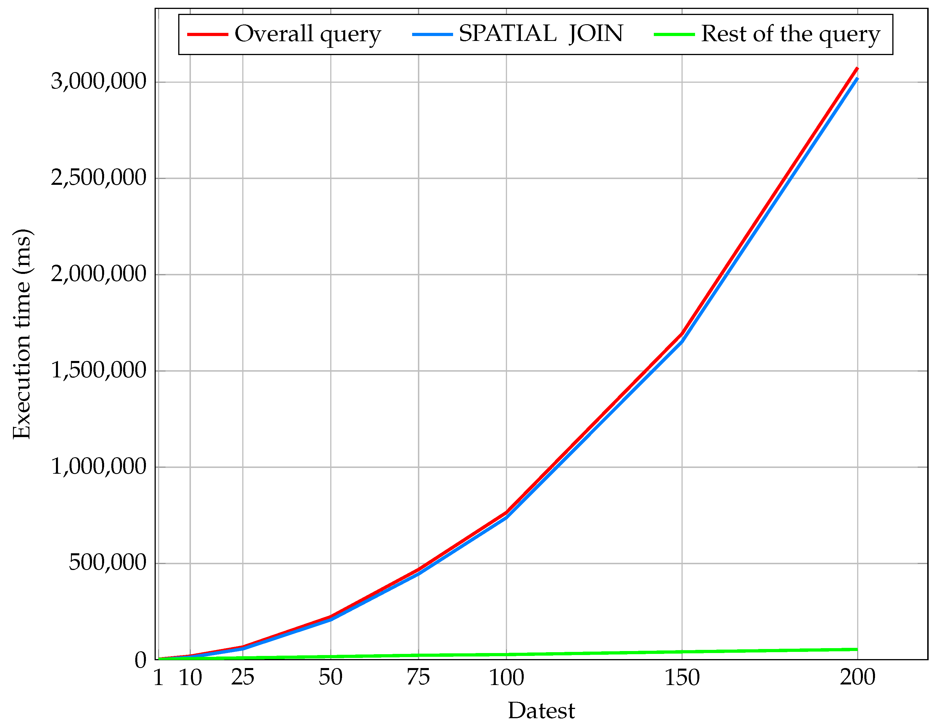
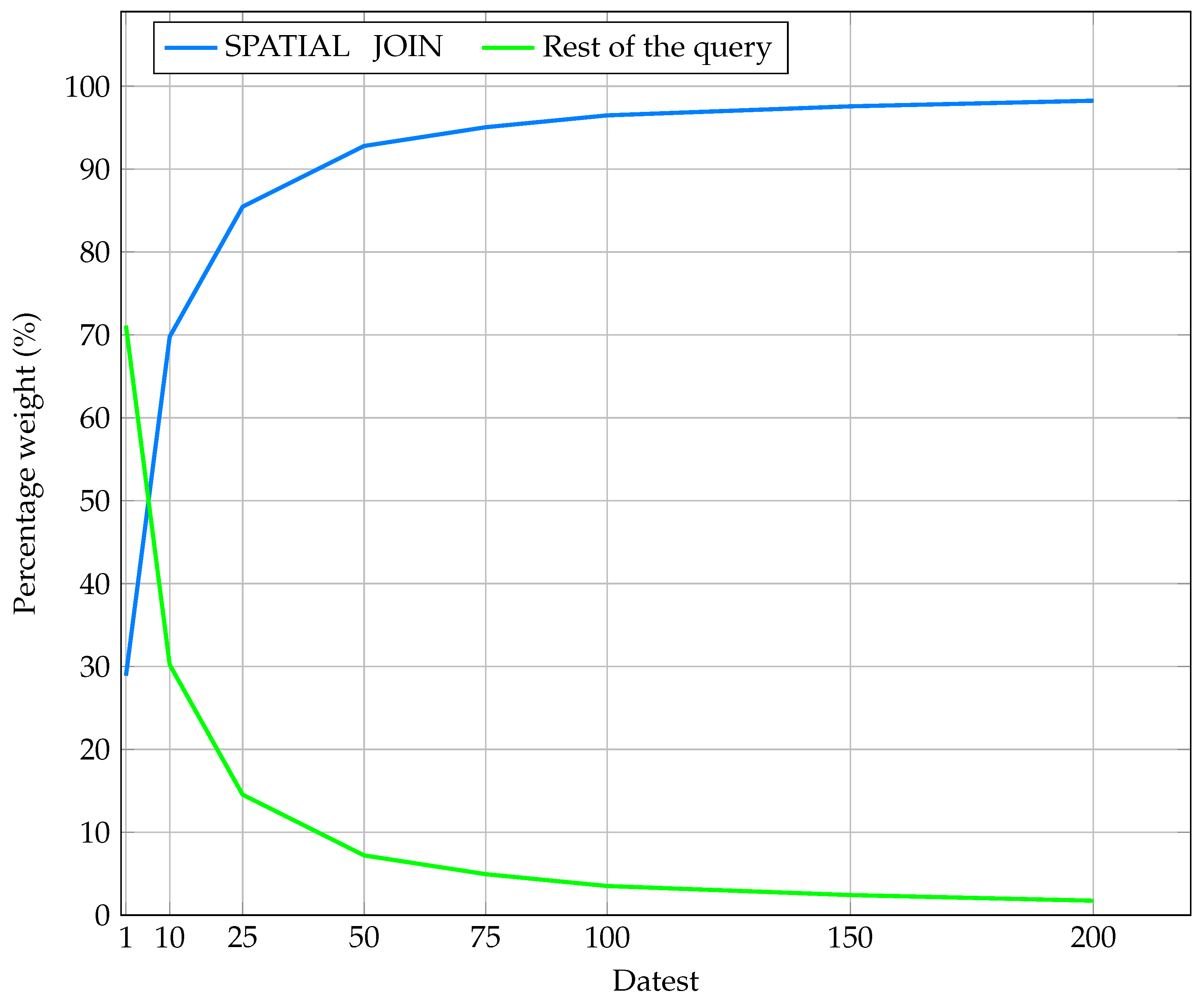
6.1. Scalability of the J-CO-QL Engine

First of all, we tested the execution of the query five times on the basic data set DS_1, in order to check for the stability of the J-CO-QL Engine.

Table 3. Execution times (in ms) for data set DS_1 on one single process of the J-CO-QL Engine.

Instruction	Avg.	Exec. 1	Exec. 2	Exec. 3	Exec. 4	Exec. 5
1. USE DB	0.31	0.99	0.31	0.16	0.04	0.03
2. USE DB	0.03	0.05	0.02	0.03	0.03	0.03
3. USE DB	0.02	0.03	0.02	0.03	0.02	0.02
4. GET COLLECTION	306.55	1,088.70	138.00	122.97	99.64	83.46
5. FILTER	2.43	9.99	0.86	0.30	0.50	0.51
6. SET INTERMEDIATE	164.39	247.16	172.25	126.64	162.62	113.25
7. GET COLLECTION	59.27	100.33	64.47	63.80	31.84	35.90
8. FILTER	220.29	409.07	241.38	150.78	143.52	156.72
9. SET INTERMEDIATE	99.56	157.43	103.85	94.21	74.21	68.09
10. SPATIAL JOIN	706.82	1,417.74	677.38	489.00	507.97	442.00
11. GROUP	5.82	18.64	3.20	2.34	2.31	2.62
12. FILTER	133.85	302.74	111.68	99.64	89.16	66.03
13. FILTER	1.58	2.72	1.70	1.46	0.93	1.06
14. SAVE AS	98.17	172.54	84.16	91.87	81.15	61.12
Total (ms)	1,799.08	3,928.10	1,599.28	1,243.23	1,193.96	1,030.84

reports the measured execution times. Rows from 1 to 14 correspond to each single instruction in the query (see Listings 3 and 4), while the bottom row reports the overall execution times. The Avg. column reports the average values of the 5 executions, while columns from Exec. 1 to Exec. 5 report times measured during each single execution.

We can notice that the overall query has an average execution time of about $1.8$ s, which is acceptable if we consider the complexity of dealing with geometries of districts, which are not simple. In fact, the most time consuming instruction is the SPATIAL JOIN, as we expected, which has an average execution time of $0.7$ s (on the overall time of $1.8$ s).

The other time-consuming instructions are GET COLLECTION, SET INTERMEDIATE and SAVE AS, although their order of magnitude is at least $2/3$ times less; in this sense, observe that the SPATIAL JOIN instruction gets collections from the $IR$ DB, which is managed though the file system, so we can consider that $0.2$ s on $0.7$ s are necessary to get the two input collections into main memory.

Comparing column Exec. 1 with columns Exec. 2 to Exec. 5, we can notice how the first execution of the query is significantly slower than the next ones, i.e., more than $3.9$ s vs. 1 s (for Exec. 5). This fact is mitigated by the average, but it is surprising: we think it is the Java Virtual Machine that during the first execution has to do extra work that is not performed during subsequent executions.

Consequently, we decided to repeat the experiment by using the DS_10 data set (see Table 2), in order to check if the above-mentioned phenomenon still appears.

Table 4. Execution times (in ms) for data set DS_10 on one single process of the J-CO-QL Engine.

Instruction	Avg.	Exec. 1	Exec. 2	Exec. 3	Exec. 4	Exec. 5
1. USE DB	0.04	0.08	0.04	0.03	0.03	0.02
2. USE DB	0.03	0.02	0.02	0.02	0.03	0.03
3. USE DB	0.02	0.02	0.02	0.01	0.02	0.01
4. GET COLLECTION	0.01	0.02	0.01	0.01	0.02	0.01
5. FILTER	5.47	20.14	3.01	1.34	1.49	1.36
6. SET INTERMEDIATE	800.51	1075.87	874.02	671.30	670.68	710.68
7. GET COLLECTION	214.74	437.30	167.66	151.11	147.97	169.66
8. FILTER	1196.96	2173.38	989.40	904.84	927.73	989.45
9. SET INTERMEDIATE	486.41	713.83	417.10	403.20	416.89	481.03
10. SPATIAL JOIN	11,475.88	16,998.58	10,088.89	10,032.71	10,074.85	10,184.37
11. GROUP	4.12	12.07	2.96	2.10	1.45	2.03
12. FILTER	70.84	128.41	56.46	56.87	56.32	56.11
13. FILTER	0.65	1.02	0.56	0.53	0.55	0.57
14. SAVE AS	82.80	144.41	87.49	58.31	57.59	66.22
Total (ms)	14,338.48	21,705.16	12,687.65	12,282.40	12,355.62	12,661.57

reports the measured execution times. We can notice that the first execution (the Exec. 1 column) is still significantly slower than next executions. However, typically users perform the same query only once, so we decided to run next experiments in a different way: we considered again 5 executions of the query, but each time the J-CO-QL Engine was shut down and restarted, so as to have the JVM in the same initial state. With such a setting, we obtained stable execution times for all 5 repetitions of the same query.

After the preliminary experiment previously discussed, we performed the experiments for all the data sets reported in Table 2, i.e., DS_1, DS_10, DS_25, DS_50, DS_75, DS_100, DS_150 and DS_200.

Table 5. Execution times (in ms) for data sets DS_1, DS_10, DS_25, DS_50, DS_75, DS_100, DS_150 and DS_200.

Instruction	DS_1	DS_10	DS_25	DS_50	DS_75	DS_100	DS_150	DS_200
1. USE DB	2	1	1	1	1	1	1	1
2. USE DB	0	0	0	0	0	0	0	0
3. USE DB	0	0	0	0	0	0	0	0
4. GET COLLECTION	951	1,598	2,368	3,726	5,177	5,733	7,966	9,831
5. FILTER	8	22	36	52	55	57	59	66
6. SET INTERMEDIATE	214	952	1,885	3,362	4,338	5,201	8,180	10,505
7. GET COLLECTION	83	374	893	1,020	1,368	1,747	2,566	3,911
8. FILTER	324	1,841	2,938	5,340	8,344	9,872	15,747	20,460
9. SET INTERMEDIATE	136	654	1,230	2,340	3,669	3,958	6,349	8,657
10. SPATIAL JOIN	857	13,095	56,513	207,209	445,508	737,696	1,652,120	3,021,693
11. GROUP	9	8	11	12	14	13	14	11
12. FILTER	228	92	125	130	121	134	103	121
13. FILTER	3	1	1	1	1	1	1	1
14. SAVE AS	153	126	130	126	127	174	118	124
Total (ms)	2,966	18,764	66,132	223,319	468,722	764,587	1,693,224	3,075,381
Total (min)	0.05	0.31	1.10	3.72	7.81	12.74	28.22	51.26
Total (min′s″)	0${}^{\prime }$03${}^{″}$	0${}^{\prime }$19${}^{″}$	1${}^{\prime }$06${}^{″}$	3${}^{\prime }$43${}^{″}$	7${}^{\prime }$49${}^{″}$	12${}^{\prime }$45${}^{″}$	28${}^{\prime }$13″	51${}^{\prime }$15${}^{″}$
SPATIAL JOIN %	28.90%	69.79%	85.45%	92.79%	95.05%	96.48%	97.57%	98.25%
Rest of the query %	71.10%	30.21%	14.55%	7.21%	4.95%	3.52%	2.43%	1.75%

reports the measured execution times (average of five executions, performed shutting down the J-CO-QL Engine after each execution). For each test, the total execution time is reported in ms in the Total (ms) row; the Total (min) row reports the same times converted to minutes (for example, $1.25$ min), while the Total (min′s″) row converts them to the form minutes and seconds (for example, 1′15″). Finally the SPATIAL JOIN % row reports the percentage of execution time taken by the SPATIAL JOIN instruction on the overall query execution time, while the Rest of the query % row reports the percentage of query execution time without the SPATIAL JOIN.

First of all, the reader can notice that instructions from 11 to 14, that are executed after the SPATIAL JOIN, are not affected by the increasing size of data sets. This is due to the fact that documents in the source collections are obtained by duplicating the original documents in the DS_1 data set. So, the spatial join would generate multiple copies of the same documents; however, the REMOVE DUPLICATES option (see Listing 4) removes duplicate documents from the output temporary collection generated by the SPATIAL JOIN instruction; thus, this temporary collection is always the same, independently of the data set.

Figure 7 plots the execution times, with respect to the size of the data sets. On the x axis, we report the multiplication factor f we used to generate each single data set. Three lines are plotted: the red line shows the overall execution times; the blue line shows the execution time taken by the SPATIAL JOIN instruction; the green line shows the overall execution time without the time taken by the SPATIAL JOIN instruction. The three lines clearly show how the execution time is dominated by the SPATIAL JOIN instruction. In fact, the rest of the query (green line) scales very well and its contribution becomes substantially negligible for the large data sets.

This behavior is further highlighted by Figure 8, which plots two curves: the blue line shows the percentage of execution time taken by the SPATIAL JOIN instruction; the green line shows the percentage of the overall execution time without the time taken by the SPATIAL JOIN instruction. The reader can clearly see how the quadratic complexity of the SPATIAL JOIN instruction dominates as long as the size of data sets increases.

Nevertheless, the reader can notice that the J-CO-QL Engine performs quite well, even with large data sets. In fact, DS_200 contains 17,600 documents in the Districts collection and 84,400 documents in the BikeLanes collection; this means that the SPATIAL JOIN instruction has to compute the intersection of geometries for 1,485,440,000 pairs and remove duplicates accordingly; it takes 50 min, which is a quite acceptable execution time, considering the size of the data set. We obtained this good performances by exploiting multi-threading, so as to exploit all the cores in the CPU. In the near future, we plan to investigate the adoption of spatial indexes computed on the fly, i.e., immediately before the execution of the SPATIAL JOIN instruction; in particular, we will have to understand the threshold above which it becomes advantageous to spend time to build spatial indexes, so as to introduce some heuristics to decide whether to use them.

We conclude this part of the experimental evaluation by considering the behavior of the FILTER instruction. To this end, we rely again on Table 5.

First of all, consider the first two FILTER instructions at line 5 and line 8, where the former selects districts, while the latter selects bike lanes. They both scale linearly. Furthermore, the execution times remain very low for the FILTER instruction at Line 5 (from 8 ms to 66 ms), while the FILTER instruction at Line 8 takes longer (from 324 ms to more than 20 s). This is due to many reasons: the first one is the fact that the BikeLanes collection contains more than 4 times documents than those in collection Districts; the second reason is that the FILTER instruction at line 8 builds the internal representation of the ~geometry field (based on the JTS Java Topology Suite library), which is expensive to do. In fact, the FILTER instruction at line 5 does not have to do that, since documents in the Districts collection already have the ~geometry field, so that their internal representation is built during the GET COLLECTION instruction at line 4. The reader can see that the GET COLLECTION instruction at line 7 is much faster than the one at line 4, because it does not have to build the internal representation of the geometry, which is done during the GET COLLECTION instruction at Line 4.

We now consider the FILTER instructions at Lines 12 and 13. Due to the fact that all data sets are obtained by cloning documents in the original DS_1 data set, the SPATIAL JOIN instruction at Line 10 produces exactly the same documents for each data set, because it removes duplicates. Consequently, the two FILTER instructions at Lines 12 and 13 should be independent of the data set. While the latter is stable and very fast (the FILTER instruction selects a very small number of very simple documents), we cannot say the same for the former one. We noticed this behavior and we investigated it. It depends on the way the Java Virtual Machine (JVM) manages main memory; strangely, it is slower with the smallest data set (228 ms) and faster with DS_10 (92 ms), while it does not exceed 134 ms in the worst case (excluded DS_1).

We can conclude this analysis stating that two main factors affect the execution times of the FILTER instruction. They are the size of the input temporary collection (as far as the number of documents is concerned) and the fact that the internal representation of geometries must be built or not. Nevertheless, its execution times are always negligible if compared with the SPATIAL JOIN instruction.

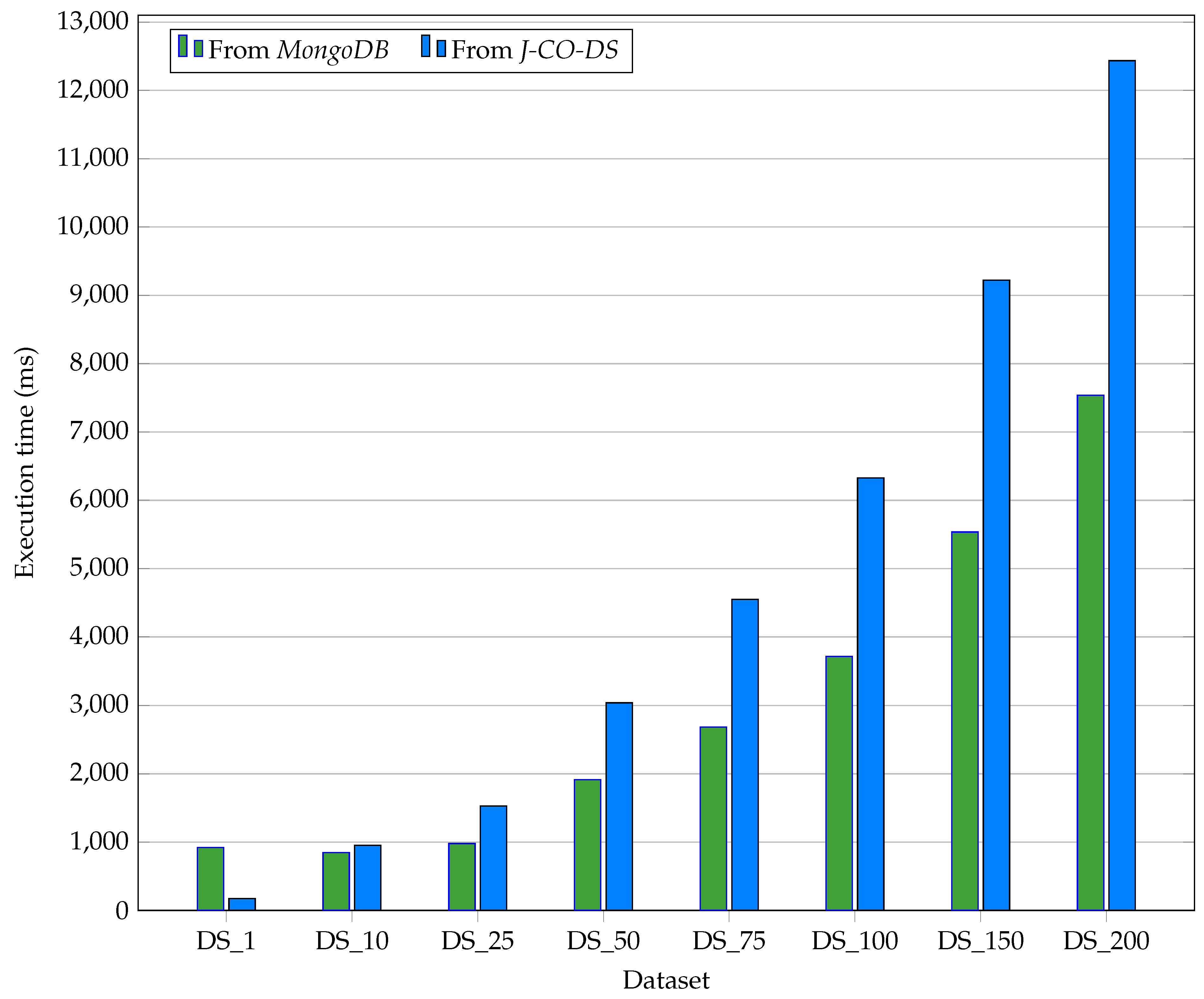
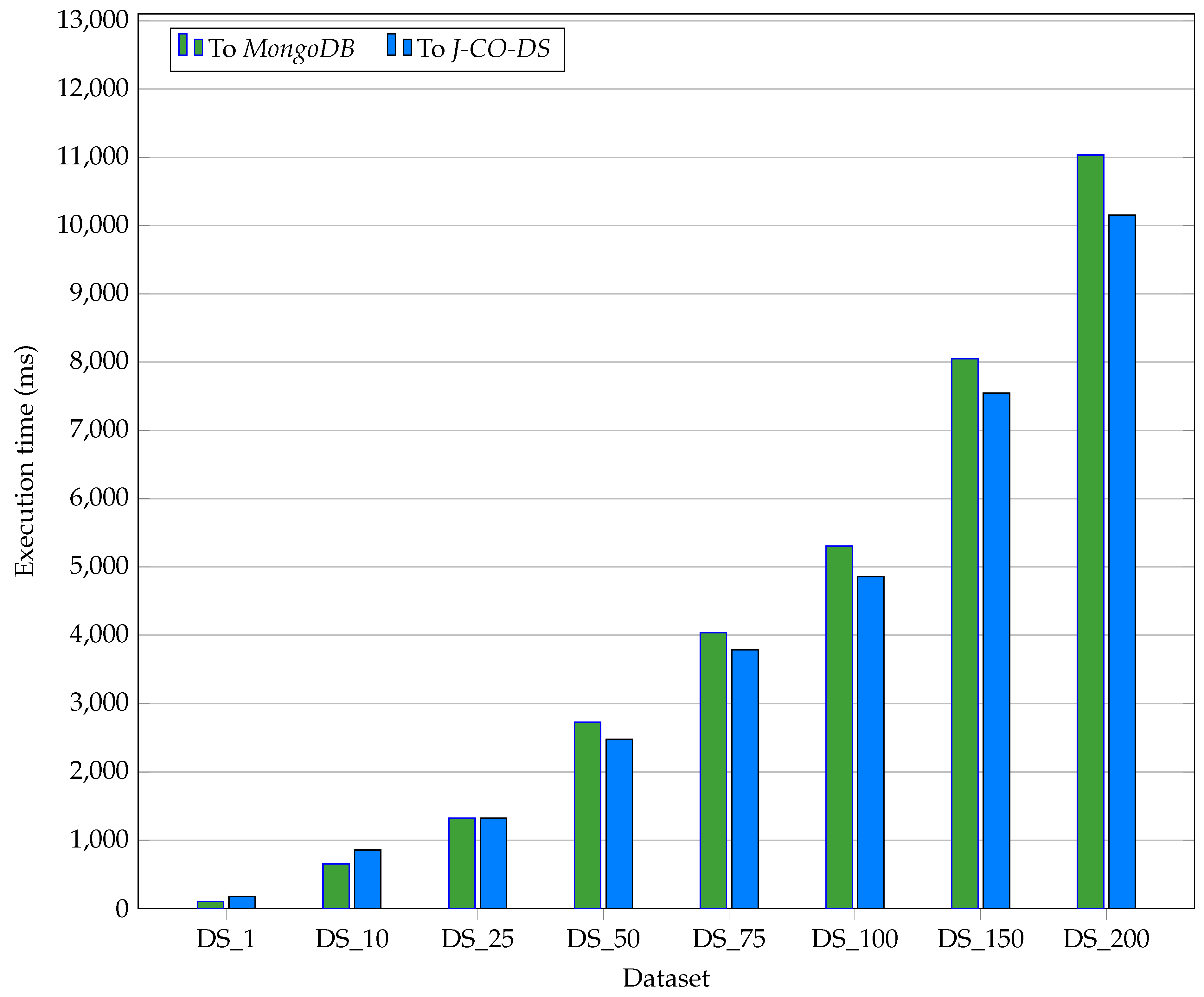
6.2. J-CO-DS vs. MongoDB

Another test we performed is comparing performance of J-CO-DS, the storage service developed as an integral part of the framework, and MongoDB.

Table 6. Performance comparison between MongoDB and J-CO-DS.

Dataset	DS_1	DS_10	DS_25	DS_50	DS_75	DS_100	DS_150	DS_200
FromMongoDB	922	847	979	1,915	2,686	3,713	5,535	7,537
FromJ-CO-DS	173	954	1,529	3,039	4,550	6,327	9,222	12,435
ToMongoDB	100	655	1,324	2,728	4,033	5,303	8,050	11,034
ToJ-CO-DS	180	858	1,325	2,480	3,784	4,856	7,547	10,154

reports the times needed to execute the GET COLLECTION instruction to retrieve the Districts collection, from the various data sets generated for the experimental campaign; once loaded, this temporary collection was saved (by means of the SAVE AS instruction) to a MongoDB database as well as to a J-CO-DS database. Table 6 reports the measured execution times. The FromMongoDB row and the FromJ-CO-DS row report the execution times (in ms) to perform the GET COLLECTION instruction from the MongoDB database and from the J-CO-DS database, respectively; Figure 9 depicts the results (the green bars correspond to tests performed on MongoDB, while the blue bars correspond to tests performed on J-CO-DS). Similarly, in Table 6 the To MongoDB row and the To J-CO-DS row report the execution times to perform a SAVE AS instruction to the MongoDB database and to the J-CO-DS database, respectively; Figure 10 depicts the results (green bars and blue bars correspond to tests performed on MongoDB and on J-CO-DS, respectively).

From Figure 9, we notice that execution times to get collections from MongoDB for the DS_1, DS_10 and DS_25 data sets are not affected by their size; probably, this is due to the time needed to connect to the database. With the other (and larger) data sets, the execution time increases linearly, as we expected. In contrast, getting collections from the J-CO-DS database behaves in a more regular way, being substantially linear for all the data sets, because J-CO-DS is based on the file system and the connection time is negligible. However, as the size of the collection increases, J-CO-DS becomes slower than MongoDB, because J-CO-DS stores collections as text files, which are larger than the BSON binary representation used by MongoDB.

Figure 10 depicts the results for writing collections to the databases. Both the databases show a regular behavior. Notice that as long as the size of the collection increases, J-CO-DS becomes a little faster. We think that this is due to the fact that documents in the collection to save to MongoDB must be converted into the BSON binary format before sending them, while J-CO-DS receives documents in the JSON text format.

So, the BSON representation gives a little advantage to MongoDB for reading collections, but at the same time it gives a little disadvantage for writing collections. Nevertheless, we can see that there are no substantial differences between the two storage systems; consequently, J-CO-DS can be effectively used in place of MongoDB to store large collections of JSON documents, without the limitation that characterizes MongoDB (single documents cannot have a BSON representation larger than 16 MByte).

7. Conclusions

We can now conclude the paper. First of all, we report the summary of the paper. Second, we discuss possible future work.

7.1. Summary

In this paper, we presented J-CO, a platform-independent framework for managing JSON data sets. The platform-independent approach is motivated by the large variety of data storage systems that could be involved in analysis activities performed by analysts (such as geographers) based on Big Data and Open Data sources, as well as social media data and volunteered information. Very often, such information is geo-tagged, because it describes features concerning territories, movements of people on the Earth globe, and so on. Consequently, the framework is oriented to (spatial) analysts and is built around a language, named J-CO-QL, that natively deals with spatial representation and provides spatial operations.

When we say that the J-CO Framework is oriented to analysts, we also mean that it is designed to support integration and cross-analysis of data coming from different JSON stores possibly powered by different technologies with various processing capabilities. It is not at all designed to support operational OLTP activities, like a classical DBMS. In fact, the J-CO Framework is not at all a database management system: it is a unifying framework for analysis activities, since it provides a platform-independent view of JSON stores and JSON data sets. Components in the J-CO Framework are loosely-coupled; storage systems, execution engines and user interfaces are possibly delocalized over the Internet and are connected each other when it is necessary. This loosely-coupled design provides flexibility and ease of cooperation among people all around the world working together by sharing data sets.

In this paper, we presented the current state of development of the J-CO Framework, which has finally become exploitable by analysts, thanks to the addition of two novel components, i.e., the data-storage service for large single JSON documents named J-CO-DS and the user interface named J-CO-UI, as well as thanks to the re-engineering of the J-CO-QL Engine. Furthermore, for the first time, we report the results of an experimental evaluation that we conducted to test scalability of the execution engine. The results show that the J-CO-QL Engine performs quite fast with small data sets and scales well with large data sets, being able to process a query based on a SPATIAL JOIN instruction on the largest data set we built in about 50 min. This fact allows us to claim that the J-CO Framework is actually suitable to work on data sets whose size is large, although we cannot talk about Big Data. We also compared J-CO-DS and MongoDB, as far as reading and writing collections are concerned: we discovered that the two storage systems have comparable performances, both when reading collections and when writing collections; consequently, since J-CO-DS does not pose any limitation to the size of documents, it is a complementary tool for storing huge JSON documents; furthermore, since J-CO-DS provides a simple interface (in that it does not provide a query language), it can be easily adopted by users that need a simple tool to store JSON data sets.

7.2. Future Work

Even though the reader could think that we are at the end of the development of the J-CO Framework, this is not true. In fact, we plan to work on the framework by following many development directions.

First of all, we will further improve the J-CO-QL Engine. The first topic we are going to address is concerned with performance. In fact, with the current stage of development we demonstrated the feasibility of the idea. Now, we are going to devise and implement specific optimizations, in particular for spatial operations: in fact, we think that the adoption of spatial indexes computed on the fly could improve the capability of dealing with very large data sets; however, due to the loosely-coupled approach (that makes the J-CO-QL Engine able to process data sets coming from JSON stores having no processing capability), as well as due to the fact that the SPATIAL JOIN can be performed on temporary collections, it is not possible to rely on pre-built spatial indexes; the engine will have to build them on the fly, task that needs additional execution time; thus, it will be important to understand when to adopt spatial indexes.

We will also investigate the possibility to integrate the J-CO-QL Engine with a Map-Reduce platform, such as Spark, that we successfully experimented for building a blind querying engine for Open Data sets [49] and for JSON data sets stored within JSON document stores [50]. In fact, in order to process actual Big Data, this solution appears to be promising; nonetheless, we will maintain the loosely-coupled approach, so as to keep user interfaces independent of computational resources actually adopted to process J-CO-QL queries.

The second topic we are going to address is the evolution of J-CO-QL. Apart from the definition of new instructions for specific analysis tasks (such as operators for performing data mining and/or machine learning tasks on JSON data sets) and location-based queries [51,52], we will try to make J-CO-QL to meet the data-independence principle. In fact, a weakness of the current proposed instructions is that users need to be aware of the structure of JSON documents; in fact, the current level of J-CO-QL is higher than traditional procedural programming languages, since its instructions are declarative, although composed in a “piped” way; so its level is not sufficiently high. In our next evolution of J-CO-QL, we aim at defining two layers of instructions: the user-layer will provide instructions that will be directly invoked by users; the hidden layer will provide instructions that will be automatically invoked by translating instructions in the user layer by a mediator. As defined in [53], “A mediator is a software module that exploits encoded knowledge about certain sets or subsets of data to create information for a higher layer of applications”: sources are encapsulated by wrappers (which access their data sources in a transparent way to mediators) to present data in the form needed by a mediator.

Finally, we argued that web sources that publish JSON data sets as well as GeoJSON documents, such as Open Data portals, could play the role of read-only JSON stores. In fact, we are planning to develop a new component to add to the framework, that will create virtual JSON stores by connecting to web sources of interest. The J-CO-QL Engine will connect to these virtual JSON stores in a seamless way: in fact, such virtual JSON stores will not have any computational capability, thus the platform-independent design will be effective for them too.

References

1. Bray, T. The Javascript Object Notation (JSON) Data Interchange Format. 2014. Available online: https://www.rfc-editor.org/rfc/rfc7159.txt (accessed on 3 March 2021).
2. Bray, T.; Paoli, J.; Sperberg-McQueen, C.M.; Maler, E.; Yergeau, F. Extensible markup language (XML) 1.0; W3C Recommendation. 2000. Available online: https://www.w3.org/TR/xml/ (accessed on 25 February 2021).
3. Butler, H.; Daly, M.; Doyle, A.; Gillies, S.; Hagen, S.; Schaub, T. The geojson format. In Internet Engineering Task Force (IETF); 2016; Available online: https://tools.ietf.org/html/rfc7946 (accessed on 25 February 2021).
4. Chow, T.E. Geography 2.0: A mashup perspective. In Advances in Web-based GIS, Mapping Services Furthermore, Applications; CRC Press: Boca Rato, FL, USA, 2011; pp. 15–36. [Google Scholar]
5. Cattell, R. Scalable SQL and NoSQL data stores. ACM Sigmod Rec. 2011, 39, 12–27. [Google Scholar] [CrossRef] [Green Version]
6. Chodorow, K. MongoDB: The Definitive Guide; O’Reilly Media, Inc.: Sebastopol, CA, USA, 2013. [Google Scholar]
7. Burini, F.; Cortesi, N.; Gotti, K.; Psaila, G. The Urban Nexus Approach for Analyzing Mobility in the Smart City: Towards the Identification of City Users Networking. Mob. Inf. Syst. 2018, 2018, 6294872. [Google Scholar] [CrossRef] [Green Version]
8. Bordogna, G.; Capelli, S.; Psaila, G. A big geo data query framework to correlate open data with social network geotagged posts. In Proceedings of the Annual International Conference on Geographic Information Science, Wageningen, The Netherlands, 9–12 May 2017; pp. 185–203. [Google Scholar]
9. Bordogna, G.; Ciriello, D.E.; Psaila, G. A flexible framework to cross-analyze heterogeneous multi-source geo-referenced information: The J-CO-QL proposal and its implementation. In Proceedings of the International Conference on Web Intelligence, Leipzig, Germany, 23–26 August 2017; pp. 499–508. [Google Scholar]
10. Bordogna, G.; Capelli, S.; Ciriello, D.E.; Psaila, G. A cross-analysis framework for multi-source volunteered, crowdsourced, and authoritative geographic information: The case study of volunteered personal traces analysis against transport network data. Geo-Spat. Inf. Sci. 2018, 21, 257–271. [Google Scholar] [CrossRef]
11. Cuzzocrea, A.; Psaila, G.; Toccu, M. Knowledge discovery from geo-located tweets for supporting advanced big data analytics: A real-life experience. In Model and Data Engineering, Rhodes, Greece; Springer: Berlin, Germany, 2015; pp. 285–294. [Google Scholar]
12. Cuzzocrea, A.; Psaila, G.; Toccu, M. An innovative framework for effectively and efficiently supporting big data analytics over geo-located mobile social media. In Proceedings of the 20th International Database Engineering & Applications Symposium, Montreal, QC, Cananda, 11–13 July 2016. [Google Scholar]
13. Bordogna, G.; Cuzzocrea, A.; Frigerio, L.; Psaila, G.; Toccu, M. An interoperable open data framework for discovering popular tours based on geo-tagged tweets. Int. J. Intell. Inf. Database Syst. 2017, 10, 246–268. [Google Scholar] [CrossRef]
14. Bordogna, G.; Frigerio, L.; Cuzzocrea, A.; Psaila, G. Clustering geo-tagged tweets for advanced big data analytics. In Proceedings of the 2016 IEEE International Congress on Big Data (BigData Congress), San Francisco, CA, USA, 27 June–2 July 2016; pp. 42–51. [Google Scholar]
15. Uddin, M.F.; Gupta, N. Seven V’s of Big Data understanding Big Data to extract value. In Proceedings of the 2014 Zone 1 Conference of the American Society for Engineering Education, Bridgeport, CT, USA, 3–5 April 2014; pp. 1–5. [Google Scholar]
16. Feng, J.H.; Qian, Q.; Liao, Y.G.; Li, G.L.; Ta, N.; Zhou, L.Z. Survey of research on native xml databases. Appl. Res. Comput. 2006, 6, 1–7. [Google Scholar]
17. Gou, G.; Chirkova, R. Efficiently querying large XML data repositories: A survey. IEEE Trans. Knowl. Data Eng. 2007, 19, 1381–1403. [Google Scholar] [CrossRef] [Green Version]
18. Haw, S.C.; Lee, C.S. Data storage practices and query processing in XML databases: A survey. Knowl. Based Syst. 2011, 24, 1317–1340. [Google Scholar] [CrossRef]
19. Kurgan, L.A.; Musilek, P. A survey of Knowledge Discovery and Data Mining process models. Knowl. Eng. Rev. 2006, 21, 1–24. [Google Scholar] [CrossRef]
20. Meo, R.; Psaila, G. An XML-based database for knowledge discovery. In Proceedings of the International Conference on Extending Database Technology, Munich, Germany, 26–31 March 2006; pp. 814–828. [Google Scholar]
21. Nayak, A.; Poriya, A.; Poojary, D. Type of NOSQL databases and its comparison with relational databases. Int. J. Appl. Inf. Syst. 2013, 5, 16–19. [Google Scholar]
22. Hecht, R.; Jablonski, S. Nosql evaluation: A us case oriented survey. In Proceedings of the CSC-2011 International Conference on Cloud and Service Computing, Hong Kong, China, 12–14 December 2011; pp. 336–341. [Google Scholar]
23. Han, J.; Haihong, E.; Le, G.; Du, J. Survey on NoSQL database. In Proceedings of the 2011 6th International Conference on Pervasive Computing and Applications, Chengdu, China, 11–13 May 2011; pp. 363–366. [Google Scholar]
24. Beyer, K.S.; Ercegovac, V.; Gemulla, R.; Balmin, A.; Eltabakh, M.; Kanne, C.C.; Ozcan, F.; Shekita, E.J. Jaql: A scripting language for large scale semistructured data analysis. Proc. VLDB Endow. 2011, 4, 1272–1283. [Google Scholar] [CrossRef]
25. Anderson, J.C.; Lehnardt, J.; Slater, N. CouchDB: The Definitive Guide: Time to Relax; O’Reilly Media, Inc.: Sebastopol, CA, USA, 2010. [Google Scholar]
26. Ong, K.W.; Papakonstantinou, Y.; Vernoux, R. The SQL++ unifying semi-structured query language, and an expressiveness benchmark of SQL-on-Hadoop, NoSQL and NewSQL databases. arXiv 2014, arXiv:1405.3631. [Google Scholar]
27. Chamberlin, D. SQL++ For SQL Users: A Tutorial. 2018. Available online: Amazon.com (accessed on 3 March 2021).
28. Florescu, D.; Fourny, G. JSONiq: The history of a query language. IEEE Internet Comput. 2013, 17, 86–90. [Google Scholar] [CrossRef]
29. Chamberlin, D. XQuery: An XML query language. IBM Syst. J. 2002, 41, 597–615. [Google Scholar] [CrossRef] [Green Version]
30. Arora, R.; Aggarwal, R.R. Modeling and querying data in mongodb. Int. J. Sci. Eng. Res. 2013, 4, 141–144. [Google Scholar]
31. Doulkeridis, C.; N∅rvåg, K. A survey of large-scale analytical query processing in MapReduce. VLDB J. The Int. J. Very Large Data Bases 2014, 23, 355–380. [Google Scholar] [CrossRef] [Green Version]
32. Goyal, V.; Soni, D. Survey paper on Big Data Analytics using Hadoop Technologies. Int. J. Curr. Eng. Sci. Res. (IJCESR) 2006, 3, 2394–2697. [Google Scholar]
33. Armbrust, M.; Xin, R.S.; Lian, C.; Huai, Y.; Liu, D.; Bradley, J.K.; Meng, X.; Kaftan, T.; Franklin, M.J.; Ghodsi, A.; et al. Spark sql: Relational data processing in spark. In Proceedings of the 2015 ACM SIGMOD International Conference on Management of Data, Melbourne, VIC, Australia, 31 May–4 June 2015; pp. 1383–1394. [Google Scholar]
34. Battle, R.; Kolas, D. Geosparql: Enabling a geospatial semantic web. Semant. Web J. 2011, 3, 355–370. [Google Scholar] [CrossRef]
35. Bordogna, G.; Pagani, M.; Psaila, G. Database model and algebra for complex and heterogeneous spatial entities. In Progress in Spatial Data Handling; Springer: Berlin, Germany, 2006; pp. 79–97. [Google Scholar]
36. Psaila, G. A database model for heterogeneous spatial collections: Definition and algebra. In Proceedings of the 2011 International Conference on Data and Knowledge Engineering (ICDKE); IEEE: New York, NY, USA, 2011; pp. 30–35. [Google Scholar]
37. Bordogna, G.; Campi, A.; Psaila, G.; Ronchi, S. An interaction framework for mobile web search. In Proceedings of the 6th International Conference on Advances in Mobile Computing and Multimedia, Linz, Austria, 24–26 November 2008; pp. 183–191. [Google Scholar]
38. Duggan, J.; Elmore, A.J.; Stonebraker, M.; Balazinska, M.; Howe, B.; Kepner, J.; Madden, S.; Maier, D.; Mattson, T.; Zdonik, S. The BIGDAWG polystore system. ACM Sigmod Rec. 2015, 44, 11–16. [Google Scholar] [CrossRef]
39. Singhal, R.; Zhang, N.; Nardi, L.; Shahbaz, M.; Olukotun, K. Polystore++: Accelerated Polystore System for Heterogeneous Workloads. In Proceedings of the 2019 IEEE 39th International Conference on Distributed Computing Systems (ICDCS), Dallas, TX, USA, 7–10 July 2019; pp. 1641–1651. [Google Scholar]
40. Hamadou, H.B.; Gallinucci, E.; Golfarelli, M. Answering GPSJ queries in a polystore: A dataspace-based approach. In Proceedings of the International Conference on Conceptual Modeling, Salvador, Brazil, 4–7 November 2019; pp. 189–203. [Google Scholar]
41. Jananthan, H.; Zhou, Z.; Gadepally, V.; Hutchison, D.; Kim, S.; Kepner, J. Polystore mathematics of relational algebra. In Proceedings of the 2017 IEEE International Conference on Big Data (Big Data), Boston, MA, USA, 11–14 December 2017; pp. 3180–3189. [Google Scholar]
42. Rantung, V.P.; Kembuan, O.; Rompas, P.T.D.; Mewengkang, A.; Liando, O.E.S.; Sumayku, J. In-memory business intelligence: Concepts and performance. In IOP Conference Series: Materials Science and Engineering; IOP Publishing: Sebastopol, CA, USA, 2018; Volume 306, p. 012129. [Google Scholar]
43. Shukla, A.; Dhir, S. Tools for data visualization in business intelligence: Case study using the tool Qlikview. In Information Systems Design and Intelligent Applications; Springer: Berlin, Germany, 2016; pp. 319–326. [Google Scholar]
44. Mora, J.M.L. Qlik Sense Implementation: Dashboard Creation and Implementation of the Test Performance Methodology. Master’s Thesis, Universidade Nova de Lisboa, Lisbon, Portugal, 2020. [Google Scholar]
45. Gormley, C.; Tong, Z. Elasticsearch: The Definitive Guide: A Distributed Real-Time Search and Analytics Engine; O’Reilly Media, Inc.: Sebastopol, CA, USA, 2015. [Google Scholar]
46. Manyam, G.; Payton, M.A.; Roth, J.A.; Abruzzo, L.V.; Coombes, K.R. Relax with CouchDB—Into the non-relational DBMS era of bioinformatics. Genomics 2012, 100, 1–7. [Google Scholar] [CrossRef] [Green Version]
47. Bortnikov, E.A.A.B.V.; Konstantinos, C.C.; Enyeart, C.A.D.C.D.; Laventman, C.F.G.; Manevich, Y.; Muralidharan, S.; Murthy, C.; Nguyen, B.; Sethi, M.; Singh, G.; et al. Hyperledger Fabric: A Distributed Operating System for Permissioned Blockchains. In Proceedings of the 13th EuroSys Conference, Porto, Portugal, 23–26 April 2018. [Google Scholar]
48. Hubert, G.; Cabanac, G.; Sallaberry, C.; Palacio, D. Query operators shown beneficial for improving search results. In International Conference on Theory and Practice of Digital Libraries; Springer: Berlin, Germany, 2011; pp. 118–129. [Google Scholar]
49. Pelucchi, M.; Psaila, G.; Toccu, M. Hadoop vs. Spark: Impact on Performance of the Hammer Query Engine for Open Data Corpora. Algorithms 2018, 11, 209. [Google Scholar] [CrossRef] [Green Version]
50. Marrara, S.; Pelucchi, M.; Psaila, G. Blind Queries Applied to JSON Document Stores. Information 2019, 10, 291. [Google Scholar] [CrossRef] [Green Version]
51. Bordogna, G.; Pagani, M.; Pasi, G.; Psaila, G. Evaluating uncertain location-based spatial queries. In Proceedings of the 2008 ACM Symposium on Applied Computing, Ceara, Brazil, 16–20 March 2008; pp. 1095–1100. [Google Scholar]
52. Bordogna, G.; Pagani, M.; Pasi, G.; Psaila, G. Managing uncertainty in location-based queries. Fuzzy Sets Syst. 2009, 160, 2241–2252. [Google Scholar] [CrossRef]
53. Wiederhold, G. Mediators in the architecture of future information systems. Computer 1992, 25, 38–49. [Google Scholar] [CrossRef]
Figure 1. Application Layers for the J-CO Framework.
Electronics 10 00621 g001
Figure 2. General approach to process collections (represented as rectangles): no processing activities on data sources.
Electronics 10 00621 g002
Figure 3. Execution trace for the sample transformation process written with J-CO-QL.
Electronics 10 00621 g003
Figure 4. Districts (black lines) and bike lanes (red lines) in Milan (Italy), described by documents in collections Milan_Districts and Milan_BikeLanes sketched in Listing 6.
Electronics 10 00621 g004
Figure 5. Main window of the J-CO-UI application.
Electronics 10 00621 g005
Figure 6. Inspection window of the J-CO-UI application.
Electronics 10 00621 g006
Figure 7. Overall query vs. SPATIAL JOIN vs. Rest of the query (execution times).
Electronics 10 00621 g007
Figure 8. Percentage weight of SPATIAL JOIN on the overall query.
Electronics 10 00621 g008
Figure 9. Performance comparison between MongoDB and J-CO-DS (for getting collections).
Electronics 10 00621 g009
Figure 10. Performance comparison between MongoDB and J-CO-DS (for saving collections).
Electronics 10 00621 g010