Co-Simulation and Data-Driven Based Procedure for Estimation of Nodal Voltage Phasors in Power Distribution Networks Using a Limited Number of Measured Data

Abstract

The paper studies the framework for the application of computational intelligence methods used for estimations in the distribution power system when a decreased number of measured data is present. Due to the lack of all measured data, the estimation of the distribution power system state is very challenging. The paper studies the application of the artificial neural network and metaheuristic optimization in synergy to solve the voltage phasors estimation problem. The proposed method uses a metaheuristic optimization technique to find virtual input data for the physical model of the network. The presented framework is based on the usage of different computational tools in co-simulation configuration. The research output is the proposed co-simulation setup for the estimation in the distribution power system using a decreased and limited number of available measured data. The estimation procedure was applied on four test distribution networks to validate the presented approach. The maximal estimation errors in voltage magnitudes and angles, using the proposed setup, are below 1.75% and 1${}^{\circ }$, respectively, without considering the measurement errors. When the measurement errors are taken into account, the proposed procedure estimates voltage magnitudes and angles with errors below 2.5% and 1.4${}^{\circ }$, respectively. In the scenario considering the consumers’ load shape, including the uncertainty range of 20%, the maximal estimation errors are below 1% for magnitude and 0.45${}^{\circ }$ for the angle taking the measurement errors in the range of 2% into account.

1. Introduction

The development of the smart grid concept (in the last decades) set additional requirements to obtain data related to the power network state. Such main data are the voltage profile of the distribution network because it represents basic information for further calculations used for the network management and control. In the power transmission system, due to a smaller number of network nodes, measurement of all, or almost all, nodal voltages is usually available. Unlike the power transmission network, in distribution networks, due to a large number of network nodes, measuring of the whole voltage profile is generally not provided. Because of no or limited measurement data, different estimation techniques have been applied to solve the problem.

The estimation method, based on smart metering, used to estimate loads and voltage profile is presented in [1]. In [2], the estimation procedure applied to the power transmission system using Phasor Measurement Unit (PMU) data is presented. The Artificial Neural Network (ANN) is used to obtain the pseudo measurements used in the estimation procedure presented in [3]. The references apply mathematical procedures for solving the estimation problem using weighted least squares (WLS). With developing computational intelligence techniques, these methods have recently been more frequently used in estimation procedures. The current magnitudes and PMU measurements are input into the data driven and ANN-based estimator proposed in [4]. The most recent studies applying the data driven procedures are presented in very interesting papers [5,6]. In [5], a Deep Neural Network (DNN) estimation procedure is developed and presented. Menke et al. [6] presented an ANN-based estimation technique using the standard multi-layered perceptron (MLP) ANN. In [7], three MLP ANN are used to estimate state variables in the distribution network using measured voltage phasors obtained by PMU. ANN outputs are nodal voltage phasors and loadability limit of the power network. ANN is used in [8] to obtain voltage profiles and losses for different combinations of distributed generation (DG) sizes and locations. Here, the input in ANN is a DG size and location based on what ANN gives to nodal voltage magnitudes. The authors of [9] used ANN to estimate the voltage magnitude in the specific network node using node powers as ANN inputs. In [10], ANN is used to estimate a voltage stability index based on PMU measurement data. The load values are used in [11] as ANN inputs to obtain the magnitude of nodal voltages as well as real and reactive losses in the power distribution network. In [12], ANN is used to obtain pseudo measurements of network loads based on historical load data, weather conditions and time of the day. An overview of different estimation techniques (classical and computational intelligence) can be found in a review article [13]. As can be seen from the aforementioned references, most studies use PMU meters (which are complex measurements) as an input for the estimation method in the case when voltage phasors are estimated. If such input data are not used for inputs, then only voltage magnitudes are estimated. The literature review points to gaps regarding the determination of sufficient measured quantities in distribution networks, complexity of estimation methods and voltage phasor estimations (based on basic measurements not using sophisticated measured devices such are PMU). Despite the intensive research, there are some research challenges, defined by the mentioned gaps, which need to be solved. The research presented here aims to overcome this gap by trying to present the procedure to obtain nodal voltage phasor based on a simple and limited number of measurements.

The main motivation for this study is to propose the estimation procedure for the distribution network voltage profile using a limited and minimal number of measured data. The research hypothesis is that voltage values and angles (the voltage phasor) can be estimated by measuring only a decreased number of the nodal voltage amount and input power in the slack (swing, reference) node. Furthermore, the problem can be solved by using different computational intelligence techniques in the synergy application. The proposed procedure is based on the computational intelligence techniques since there is a lack of measuring data in the power distribution networks. The co-simulation setup between a tool for power system analysis and computational intelligence methods is used in the research. The presented paper aims to use the basic measured data (because of easily available and cheap measuring devices) and as simple configurations of the computational intelligence techniques used in the framework as possible. The proposed data driven and a co-simulation-based procedure tries to contribute to decreasing the mentioned research gaps.

The rest of the paper is organized as follows. In Section 2, the computational intelligence techniques and simulation tools used in the study are briefly described. Section 3 gives an overview of the proposed estimation method. In Section 4, the application of the estimation procedure on the test power distribution systems is presented. In this section, the obtained results are commented on. At the end, the conclusion is made in Section 5.

2. A Brief Overview of the Used Computational Intelligence Techniques

Two different methods of computational intelligence were used in the study: a metaheuristic optimization method and a simple MLP ANN. Since one of the study motivations is to apply the co-simulation approach, the existing tools for these two methods were used. Instead of detailed descriptions, a short overview of these computational intelligence methods is given below because they are very well described in the literature and not developed but only used here. The tool for power system analysis was applied to generate training and testing datasets. The power system analysis tool uses a physically-based mathematical model of the power system unlike ANN which implements a nonphysical based model.

2.1. Metaheuristic Optimization Method and Computing Tool

MIDACO (Mixed Integer Distributed Ant Colony Optimization) solver [14] is an optimization tool that has an interface related to different programming environments (C/C++, Python, Julia, MATLAB, etc.). The MIDACO tool can be used for the general type of an optimization problem, i.e., continuous (linear (LP) and nonlinear (NLP)), integer (discrete) (IP) and mixed-integer (MINLP) problems. Optimization problems that can be solved using MIDACO include unconstrained and constrained problems as well as single objective (SOOP) and multi-objective optimization problems (MOOP). Owing to its interface for different programming languages and applicability for a general type of an optimization problem, the MIDACO tool is very suitable to be used in the co-simulation approach used in the research. The MIDACO tool implements the metaheuristic optimization method Ant Colony Optimization (ACO) [15]. In the MIDACO solver, the solution candidate from the problem-solution space is generated using kernels with a radial basis function. The function used for kernels is a Gaussian function and kernels correspond to the pheromones in ACO. Using the kernel function, the pheromones intensity defining the probability to move/keep ants (solution vector x) in the promising area in the solution space [15]:

$$G^i\left(x\right)=\sum _{l=1}^k(w_l^j{g}_l^j\left(x\right))=\sum _{l=1}^k{w}_l^i\frac{1}{{\sigma }_l^i\sqrt{2\pi }}{e}^{-\frac{{(x-{\mu }_l^i)}^2}{2{\left({\sigma }_l^i\right)}^2}},$$

(1)

The kernel parameters w (weight), $\mu$ (mean) and $\sigma$ (standard deviation) are updated during the optimization process according to the procedure given in [15]. The MIDACO solver has 12 parameters whose numbers of ants and kernels are tuned during the research.

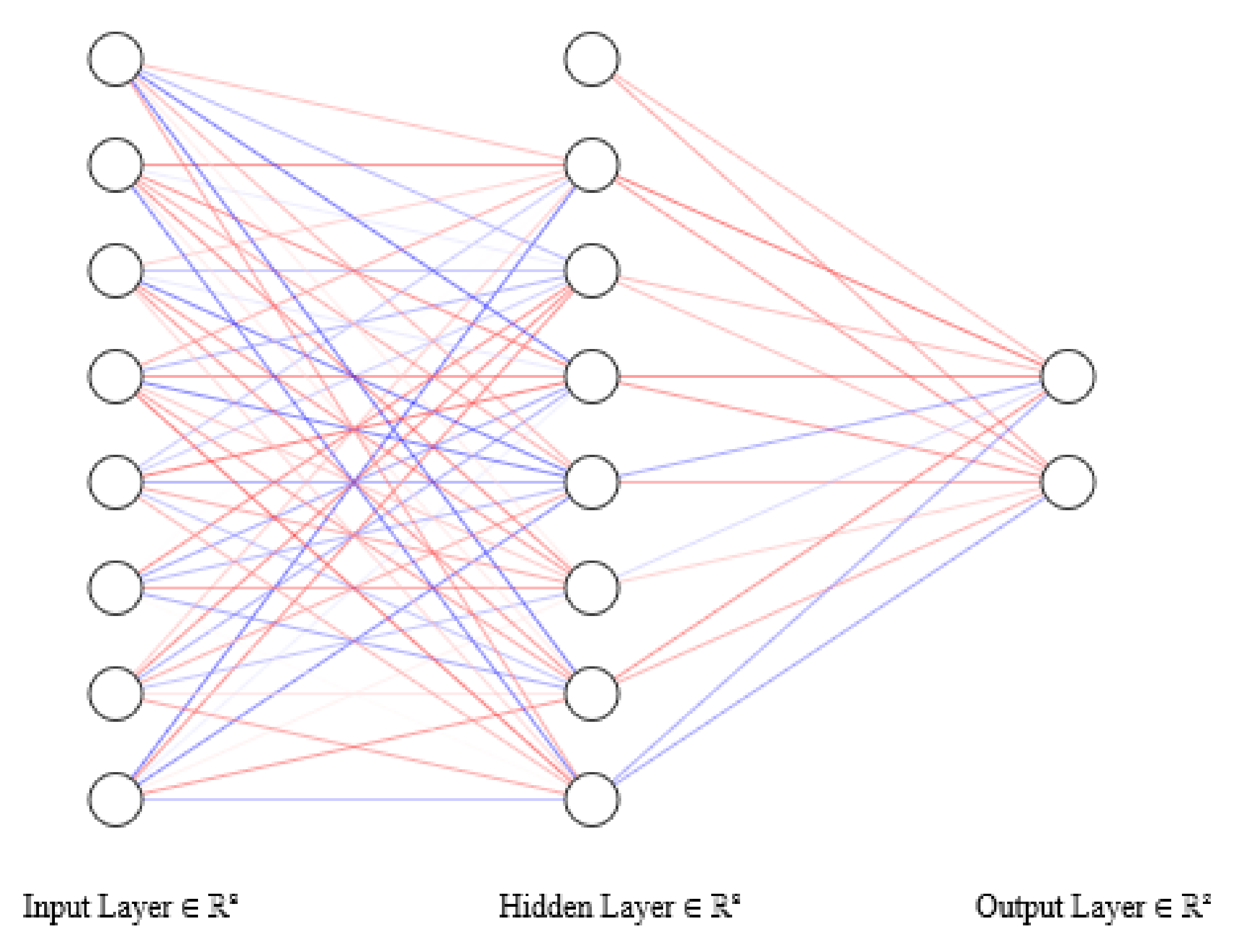
2.2. ANN Configuration and Computing Tool

One simple and very basic MLP ANN configuration contains input, one hidden and output layer (Figure 1).

This is basic feedforward ANN whose training and calculation procedures are very well developed and known. The ANN outputs from hidden and output layers are obtained by multiplying input values vector of the layer and weighting matrix. ANN has also a hyperparameter defining configuration and parameter values in the ANN structure. Some of the most important parameters are activation functions for each layer, optimization algorithm for training, learning rate and the number of neurons in the hidden layer. The Tensorflow computational tool [17] was used to implement ANN in the voltage estimation procedure. The Keras application programming interface (API) [18] for Tensorflow (TensorFlow.Keras module in Tensorflow 2 version) tool was used to easily build ANN.

2.3. A Computational Tool for Analysis of the Distribution Network

Similar to the two above tools, it is required to have a programming environment for this tool. One of such tools used here is OpenDSS (Open Distribution system Simulator) [19] which can be interfaced to Matlab, Python, C++, VBA, etc. The power network representation in OpenDSS is made by a simple textual script (OpenDSS script), and it is very easy to get, change and set properties of OpenDSS objects from outside the tool. The tool provides different types of calculations such as unbalanced power flow, fault analysis, harmonic analysis in the power system. OpenDSS simulates the power system in the phasor (frequency) domain.

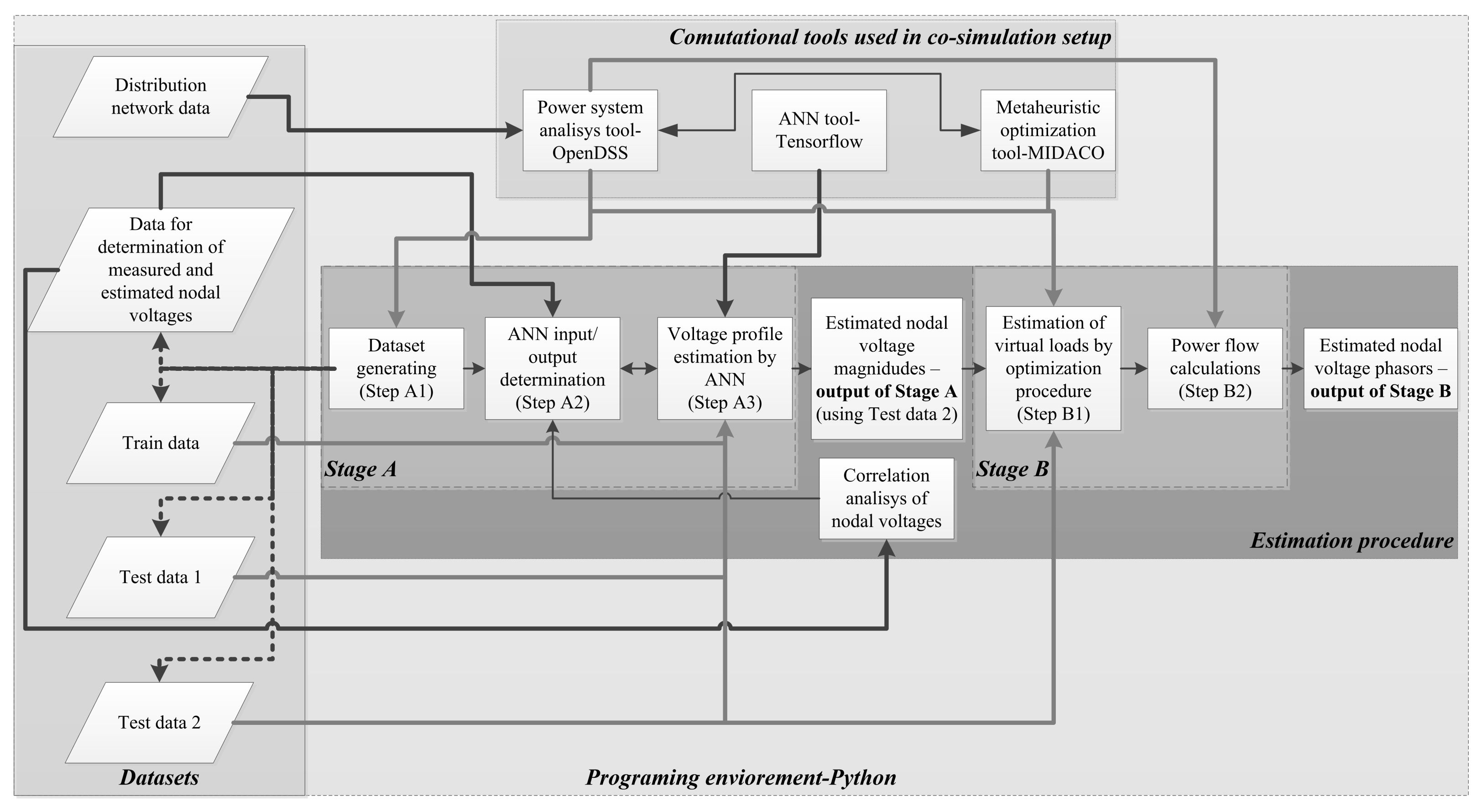
3. The Proposed Framework for the Voltage Phasor Profile Estimation

The proposed framework for the voltage phasor profile estimation is divided into two stages, denoted here as Stage A and Stage B (Figure 2).

The first stage (Stage A) deals with data preparation and ANN configuration for estimating network quantities. Stage A consists of three steps. The first step (A1) is preparation of data required for ANN training and testing as well as input data used in Stage B. The procedure for defining measured and estimated quantities is included in the second step (A2). The third step (A3) performs the ANN building, training and testing, thus resulting in prepared ANN (configured, trained and tested) to be applied in Stage B. Stage B has two steps. The first one (B1) performs the metaheuristic optimization to obtain adequate load combinations in the network. Step B2 estimates the network voltage profile based on the results obtained in Step B1 using the physical-based model of the distribution network. The overview of the framework steps is given in Figure 2 showing the interactions between the used simulation tools in the co-simulation setup.

3.1. Data Preparation—Step A1

ANN performance highly depends on the type of input and output data (among other things). For the generation of relevant dataset, mathematical formulation of the physical network model was used. The set was generated by making different combinations of the loads in the network. The samples of input data for the estimation procedure are obtained for the randomly generated network loads. Each load (active power $P_i$ and reactive power $Q_i$) is independently generated (as a fraction of the nominal powers $P_{i,N}$ and $Q_{i,N}$) to map a more general case of loads change in the real situation:

$$c_i=rand(0,1),P_i=c_i{P}_{i,N},Q_i=c_i{Q}_{i,N},$$

(2)

This generation of load combinations is more general than using the load factor on the network level or the load shapes, consequently reflecting a more realistic scenario, which can occur in real situations. Thanks to the usage of the network simulation tool (OpenDSS software in this case), different datasets such as nodal voltages (the network voltage profile), total network losses, input power in the slack node, currents in the network line segments and power flows in network line segments (one and three phases) can be obtained. Based on these datasets, different quantities can be used as inputs/outputs for ANN. During the estimation procedure, four independent datasets are generated: one as input for Step A2, two (for training and testing) as input for Step A3 and one as input for Step B1. The number of different load combinations (obtained according to (2)) was determined by applying the next rule (the rule is experimentally defined during the research) based on the number of the one-phase network node ($N_{1f}$): input for Step A2 is $50\times N_{1f}$, input for Step A3 is training $100\times N_{1f}$, input for Step A3 is testing $500\times N_{1f}$ and input for Step B1 is $500\times N_{1f}$.

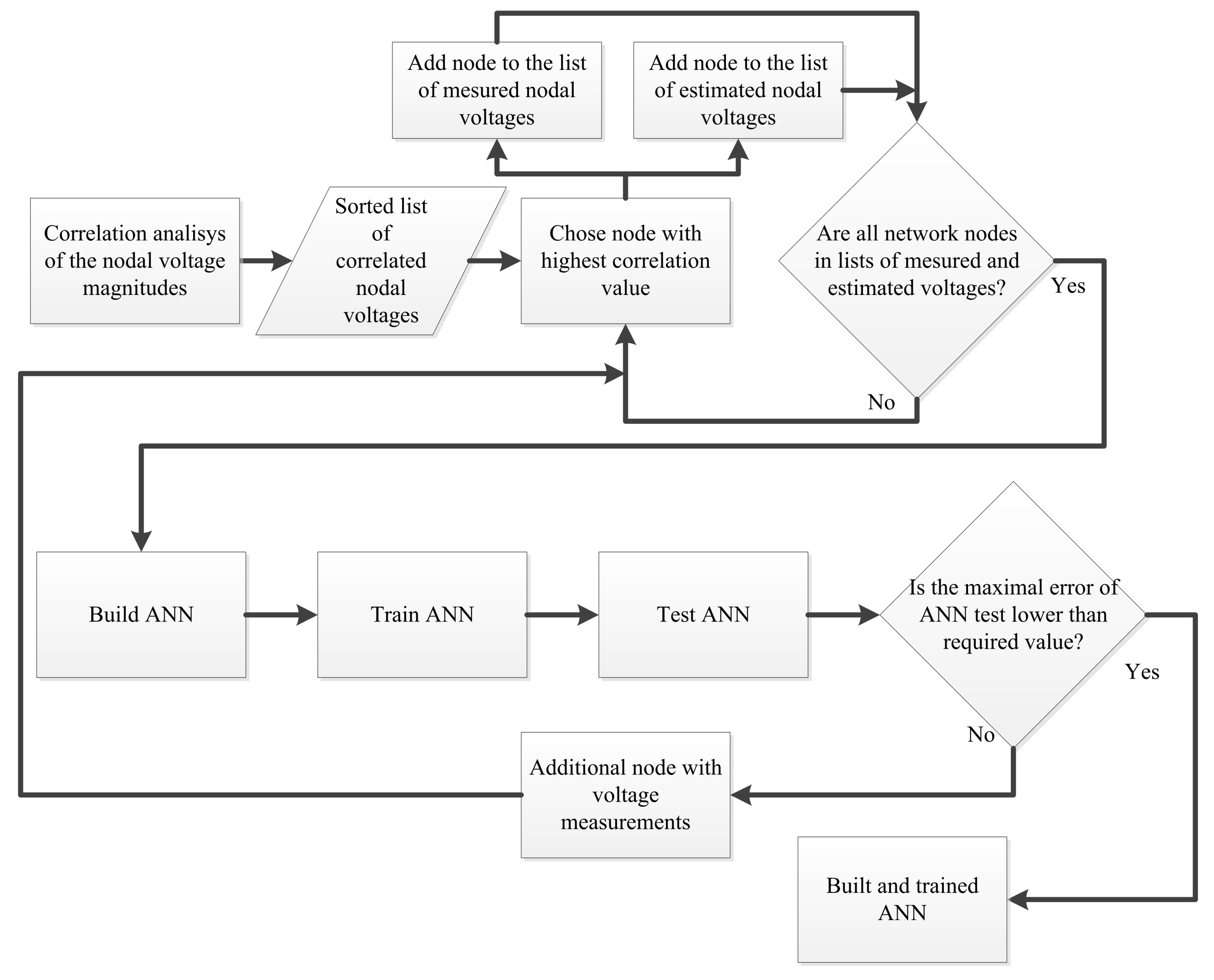
3.2. Determination of Measured and Estimated Quantities—Step A2

The analysis of different input/output combinations was done during the research aiming to meet the predefined requirements of decreasing the number of simple measurements and conducting simple ANN configuration. The process of determining the dominant input data for ANN was performed as an important factor for ANN application [20]. The input/output combinations investigated during the research were the section currents/section currents, section currents/loads, section currents/nodal voltages, nodal voltages/loads and nodal voltages/nodal voltages. Based on the analysis of the researched ANN input/output combinations, the conclusion is that the nodal voltages/nodal voltages case best meets the defined research goals. Upon defining a suitable type of physical network quantities for ANN input/output, the procedure for determining the dominant input data was performed. The procedure outcomes are network nodes with voltage measurements (ANN inputs) and voltage estimations (ANN outputs). The goal is to find the lowest possible number of measured nodal voltages that are highly correlated to the rest of nodal voltages in the distribution network. This procedure is based on the statistical technique to obtain the correlation between ANN inputs and outputs. The input data generated according to (2) have no Gaussian distribution due to the usage of uniform distribution for random number generation. Because of this and nonlinear dependence between ANN inputs and outputs, non-parametric correlation techniques need to be used instead of parametric (Pearson’s correlation) correlation methods [21]. One of the rank correlation methods, namely Kendall’s rank correlation [22], is used here. According to Corder and Foreman [21], the relationship strength of variables is strong/large and direct if the correlation coefficient is above 0.5. Upon calculating correlation coefficients between every two nodal voltages, the measured voltages are chosen on the criterion of strongly correlating with as many other nodal voltages as possible. In this procedure, network nodes are sorted in descending order according to the value of the correlation coefficients corresponding to the nodal voltage/nodal voltage relationship. There are two lists of network nodes generated in this procedure—the list of nodes with and without voltage measurements. The list of network nodes with voltage measurements is first completed with the highest correlation coefficient nodes. The list of nodes without measurements is populated with nodes correlating to nodes in the node list with measurements. At the end of this process, network nodes with voltage measurements and voltage estimations (without measurements) will be determined. The process in this step is performed simultaneously with the next step (Step A3) as described below.

3.3. Building, Training and Testing of ANN—Step A3

One of the research goals is to simplify the used computational intelligence method, as mentioned in the Introduction. In this sense, a very simple (basic) configuration of ANN consists of input, one hidden and output layer (Figure 1). The numbers of input and output neurons are defined by the numbers of network nodes with and without measurements, respectively. The hidden layer has the same number of neurons as the input layer. The error of estimated voltage values by ANN is highly impacted by the number of measured voltages. On the other hand, there is a request for a decreased number of measured values (one of the defined research goals). The limitation of the estimation error was defined to find the trade-off between these two conflicting requirements. This limitation can be expressed as the requirement that the maximum estimation error $\Delta V_{max}$ is below the given error limit $ϵ$:

$$\Delta V_{max}\le ϵ,$$

(3)

The process of ANN building and determination of network nodes with and without voltage measurement partly includes Step A2, as presented in Figure 3.

Owing to the proposed approach, the network observability has been kept low (which is one of the research goals) with a satisfying low estimation error. The observability factor can be defined as the ratio of the number of voltage measurements ($N_m$) and all nodal voltages ($N_{all}$) in the network [5]:

$$O=\frac{N_m+3}{N_{all}},$$

(4)

The addition of the number 3 in (4) represents the measurement of total power per phase in the network slack node as explained in the next section. The observability factor defined by (4) is related only to the measured quantity. However, the whole procedure estimates the nodal voltage phasors, and, since the two data (magnitude and angle) need to be measured to get the phasor, the observability factor can be defined in that case as:

$$O_{ph}=\frac{N_m+3}{2N_{all}},$$

(5)

The outcome of the first stage (Stage A) is trained ANN for estimating nodal voltage magnitudes in the network node without measurements using the measured nodal voltage magnitudes for decreased observability of the distribution network. If there are voltage regulators or on load tap changer transformers, their tap positions are assumed to be known or measured as well.

3.4. Obtaining the Virtual Loads for Voltage Phasor Estimation—Step B1

With trained ANN obtained in the previous procedure stage, the network voltage profile can be estimated for voltage magnitudes. The next procedure stage has the role of estimating the whole voltage phasor. The first step in this stage does the optimization process to obtain the network load values, which are further used in the estimation procedure. The optimization problem was defined with network loads as optimization decision variables. The nodal voltage magnitudes and total power are used to formulate the optimization objective function. The mathematical formulation of the optimization problem is given by:

$$\begin{array}{c}\hfill F\left(x\right)=\sum _{i=1}^{N_{all}}|(V_{i,m}-V_{i,e})|+\sum _{j=1}^3\left|(P_{j,m}-P_{j,e})\right|\stackrel{x_{opt}}{\to }min\\ \hfill \mathrm{subject}\mathrm{to}\mathrm{box}\mathrm{constraints}:x\in \{x_{lb},x_{ub}\}\\ \hfill \mathrm{subject}\mathrm{to}\mathrm{inequality}\mathrm{constraints}:\\ \hfill V_{min}\le V_{i,e}\le V_{max},I_{k,e}\le I_{k,max},|V_{i,e}-V_{i,m}|\le ϵ\\ \hfill \mathrm{with}\mathrm{decision}\mathrm{variables}:\\ \hfill x=[P_1,Q_1,\cdots ,P_i,Q_i,\cdots ,P_n,Q_n],\end{array}$$

(6)

where $V_{i,m},V_{i,e},P_{j,m}$ and $P_{j,e}$ are measured and estimated (by Step A3) voltage magnitudes and power (in the slack network node), respectively, $I_{k,e}$ is calculated current in the network line sections and $P_i$ and $Q_i$ are load values in the network nodes with loads. The simulation tool (Section 2.3) was used to calculate the objective function and constraint values in (6). The metaheuristic optimization method described in Section 2.1 was used to solve the optimization problem (6). The outcome of this procedure step are the values of the loads making the nodal voltage magnitude close to their measured and values estimated in Step A3. As shown below, this procedure can find load combinations different from the real one; however, that gives not only nodal voltage magnitudes but also nodal voltage phasors very close to their real values. Based on this research outcome, the load values obtained in this procedure step are called virtual load values. During the research, the next interesting cognition was reached. Different load combinations can give very close nodal voltage values. This implicates that the optimization problem (6) has many local optimums close to the global optimum.

3.5. Estimation of Nodal Voltage Phasors—Step B2

This is the final step of the proposed procedure. In this step, the simulation tool (Section 2.3) is applied by using virtual load values obtained in the previous step. The usage of the physically-based network model and obtained virtual load values complete power flow calculation. Consequently, the values of different quantities (network losses, line currents, etc.) in the network can be obtained, although the estimation procedure was designed to estimate only nodal voltage phasors.

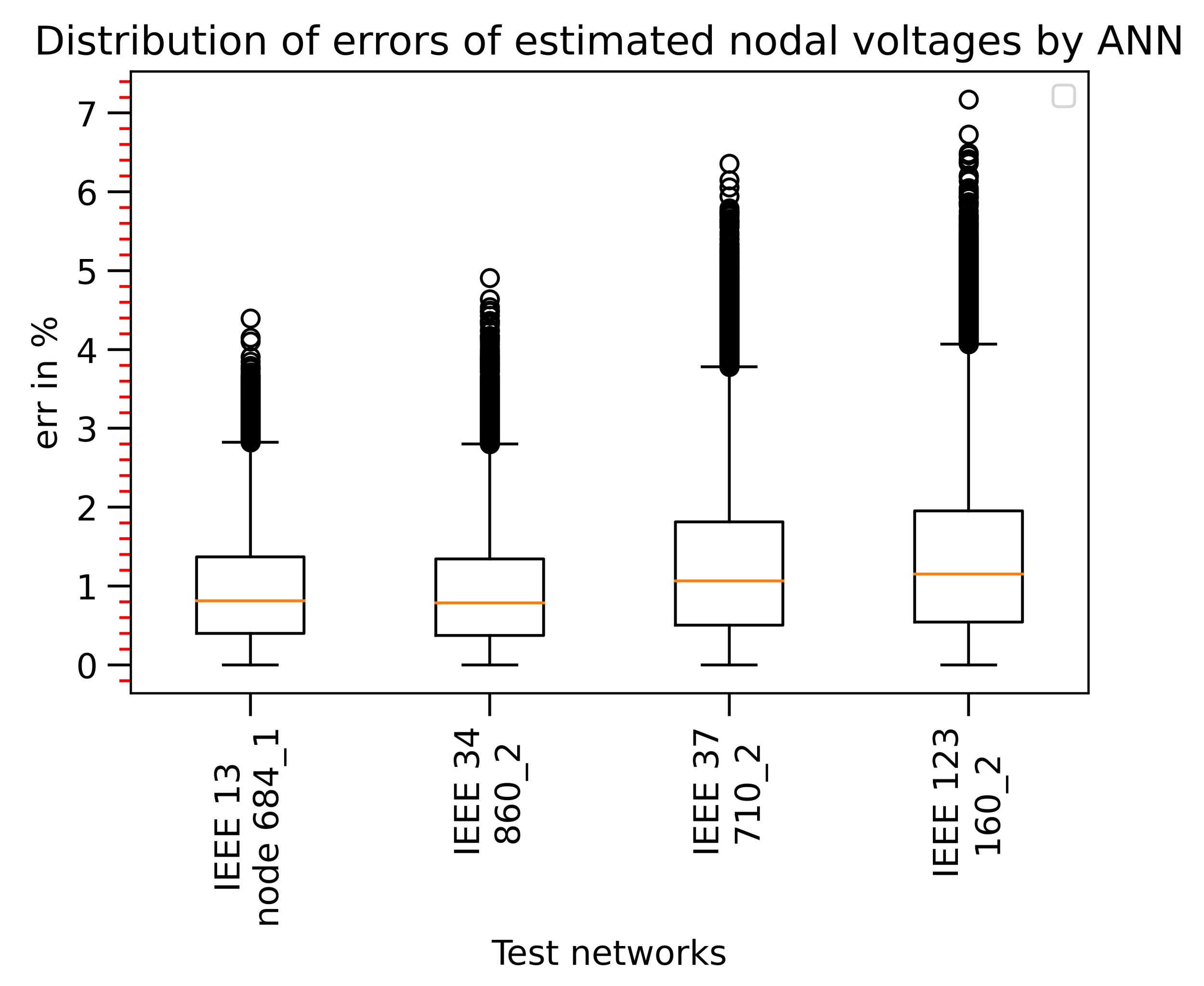
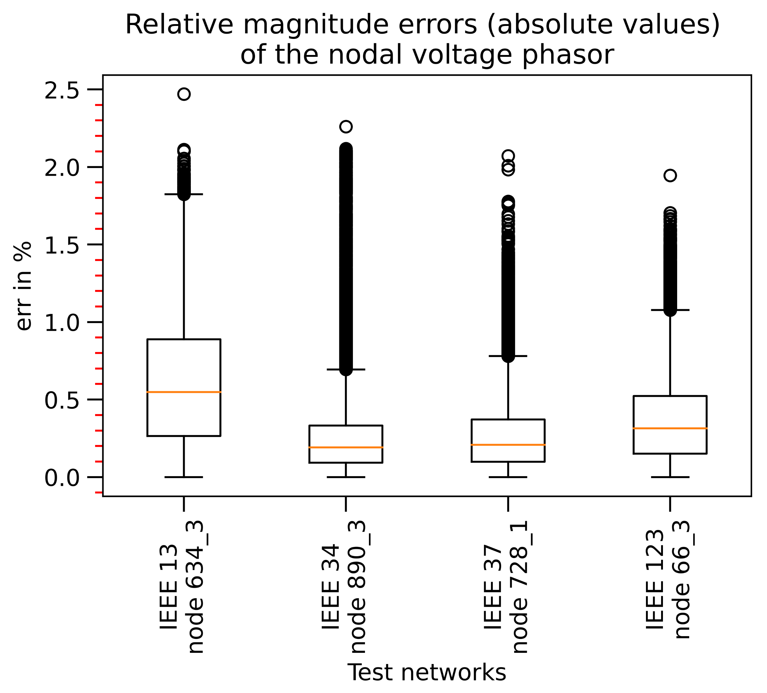
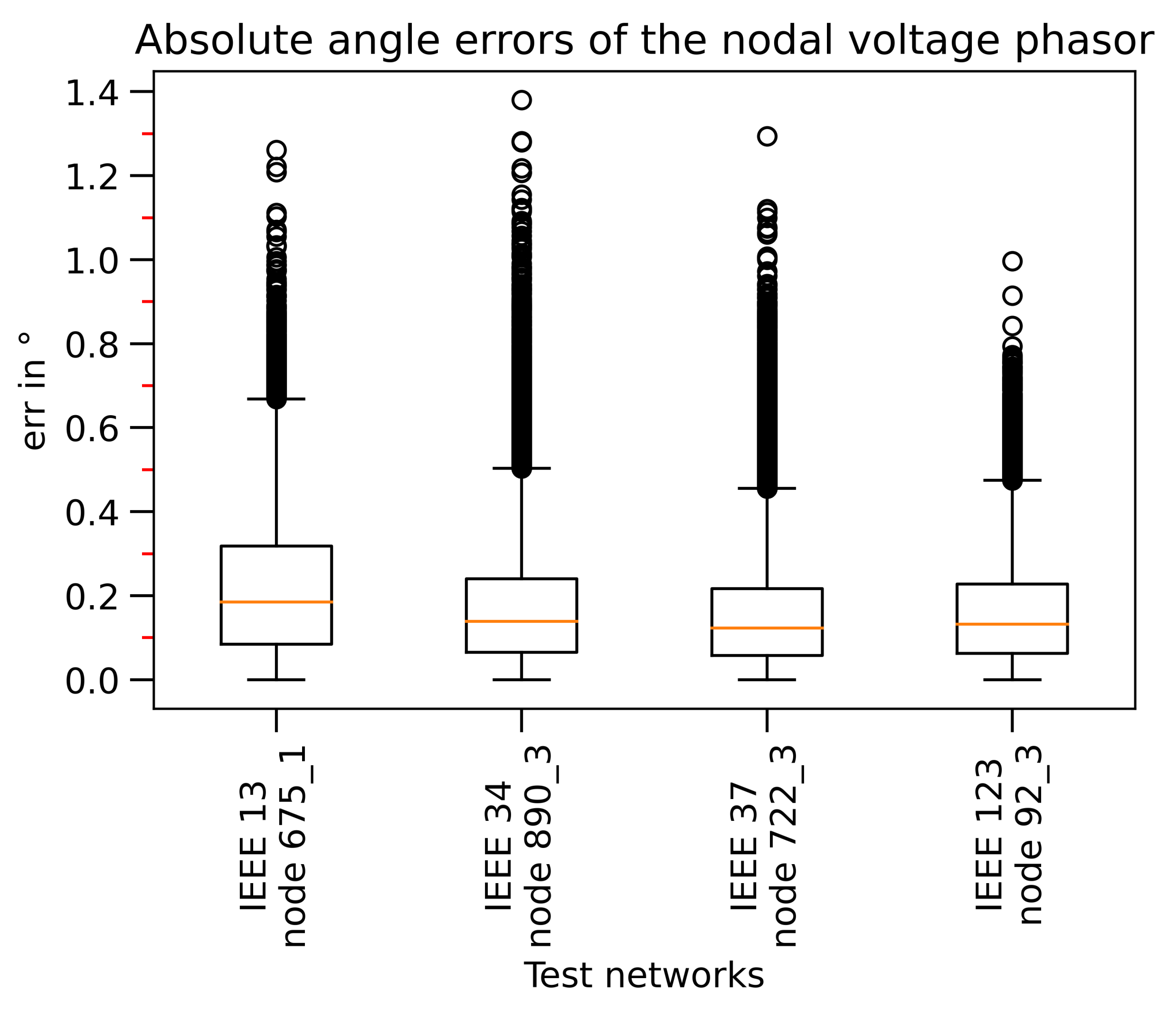
4. Obtained Results for Test Distribution Networks

The proposed framework was applied to four very common IEEE test distribution networks, namely 13, 34, 37 and 123 bus systems [23]. Since IEEE test networks are very well known, a detailed description is omitted here. A brief overview of the main features of each test network is given. The IEEE 13 node feeder is a fully unbalanced network with 1, 2 and 3 phase lines and loads (different load models: constant power, impedance and current). The feeder has several laterals. The IEEE 34 node system balances spot three-phase and distributed one-phase loads with three- and one-phase lines. The IEEE 37 and 123 node feeders are the unbalanced systems with spot loads modeled by different load models. The overview of the numbers of one-phase network nodes and loads (balanced three-phase loads are counted as one load) is given in

Table 1. Numbers of the network nodes and loads for the tested networks.

Test Network	IEEE 13	IEEE 34	IEEE 37	IEEE 123
number of 1-phase nodes	41	91	111	278
number of loads	15	52	47	98

and configurations of the tested networks in Figure 4.

Since the used computational intelligence techniques in the proposed procedure are not deterministic but have stochastic character, many different load combinations are required to test and validate the framework. The sizes of the input data for the specific procedure step are shown in

Table 2. Input dataset sizes used in the simulations.

Test Network	${\mathit{N}}_{1\mathit{f}}$	Input in A2	Input in A2 Training	Input in A2 Testing	Input in B1 and B2
IEEE 13	35	1750	3500	17,500	17,500
IEEE 34	89	4450	8900	44,500	44,500
IEEE 37	111	5000	11,100	55,500	55,500
IEEE 123	272	5000	27,200	136,000	136,000

based on the rule defined at the end of Section 3.1.

The numbers of network nodes with and without measurements (determine the number of neurons in hidden and output ANN layers, respectively) of the voltage amplitude as well as the observability factors ((4) and (5)), are given in

Table 3. Number of measured ($N_m$) and estimated ($N_e$) one-phase voltages and observability factors for tested networks.

Test Network	${\mathit{N}}_{1\mathit{f}}$	${\mathit{N}}_{\mathit{m}}$	${\mathit{N}}_{\mathit{e}}$	O	${\mathit{O}}_{\mathit{ph}}$
IEEE 13	35	17	18	0.57	0.29
IEEE 34	89	18	71	0.24	0.12
IEEE 37	111	17	94	0.18	0.09
IEEE 123	272	26	246	0.11	0.05

.

After performing Step A3, where the nodal voltage magnitudes were estimated by ANN. The obtained estimation errors are presented in

Table 4. Maximum and average percentage errors (absolute amounts) for estimated nodal voltage magnitudes (Step A2).

Test Network	${\mathit{err}}_{\mathit{max}}$ in %	${\mathit{err}}_{\mathit{mean}}$ in %
IEEE 13	1.34	0.95
IEEE 34	0.92	0.57
IEEE 37	1.06	0.71
IEEE 123	1.16	0.72

.

In Figure 5, the distributions of errors for tested networks in nodes with the highest errors are shown.

After the nodal voltage magnitudes estimated in Step A3, Stage B started. The estimated voltage magnitudes from the previous step were involved in the objective function (6) and the virtual loads were obtained by performing Step B1. In this step, very interesting and unexpected results were achieved. During the research, it was noted that the optimization procedure can find different load combinations that move nodal voltage magnitudes very close to the given values. This indicates that the optimization problem (6) has more local optimums close to objective function values. This means that the optimization problem is difficult to solve because there is a high possibility the algorithm is stuck in the local optima. Upon analysis, it was noted that the loads found by the optimization are different from the real ones. However, the voltage profile produced by estimated loads is very close to the one produced by real loads. This is a more interesting finding since there are more different load combinations that voltage profiles very close to each other can give. This incidental and unexpected conclusion was drawn from the research. To visualize this conclusion, the examples of the estimated and real load values as well as corresponding voltage profiles for the IEEE 13 node test network are shown in Figure 6. Similar results are obtained for all tested networks.

In the final step of the proposed procedure, Step B2, the virtual load combination obtained in the previous step (Step B1) was used as input resulting in a complete power flow solution. Thanks to the usage of the physically-based network model and power flow calculations, not only nodal voltage phasors (which was the main research goal) but other quantities, such as network losses and currents in the lines, can be obtained.

In Figure 7, the distribution of relative errors (absolute amounts) for nodes with the biggest errors (for each tested network) is shown. As shown in the figure, the highest errors do not exceed 1.7% of the voltage phasor magnitude for all used distribution test networks. A very high number of different load combinations (last column in Table 2) was used, and it is interesting to see error distribution in Figure 7. For all tested networks, the mean of the errors is below 0.5% and, for 75% (the third quartile) of data, the error is below 0.7%. Consequently, in the majority of cases, the magnitude voltage error is below 0.7%, 0.5%, 0.6% and 0.6% for IEEE 13, 34, 37 and 123 node test feeders, respectively. This applies to nodes with the highest errors while other nodes have even lower errors.

The absolute angle errors are given in Figure 8. In this case, the absolute values are shown instead of the percentage error since the referent phase has a phase angle of 0${}^{\circ }$. Due to this, even a small absolute error will result in a high percentage error. For two other phases (with phase shift angles of 120${}^{\circ }$ and −120${}^{\circ }$) there is no such numerical problem, e.g., the absolute error of 0.2${}^{\circ }$ will result in a percentage error of about 20% for the referent phase and about 0.17% for the two other phases. The maximum phasor angle error is below 1.15${}^{\circ }$ (IEEE 37 node test feeder) and below 0.4${}^{\circ }$ in 75% of tested cases.

The procedure was performed on the desktop PC equipped with i7-10700 CPU, 16 GB RAM and SSD storage. Python version 3.8.5, Tensorflow version 2.3.1. for CPU and MIDACO version 5 were used. The computational times for the ANN training (for the number of data given in Table 2) in Step A3 and the optimization in Step B1 are presented in

Table 5. Computational times of ANN training and optimization.

Test Network	t in s, ANN Training	t in s, Optimization
IEEE 13	26.88	1.07
IEEE 34	37.07	2.65
IEEE 37	53.32	1.92
IEEE 123	159.07	5.27

. The ANN training was performed using 2500 epochs and optimization by MIDACO with 100 ants, 10 kernels and 5000 maximum number of function evaluation. The time spent for the optimization process is given per one input data pattern because in the procedure implementation one sample of input values is used.

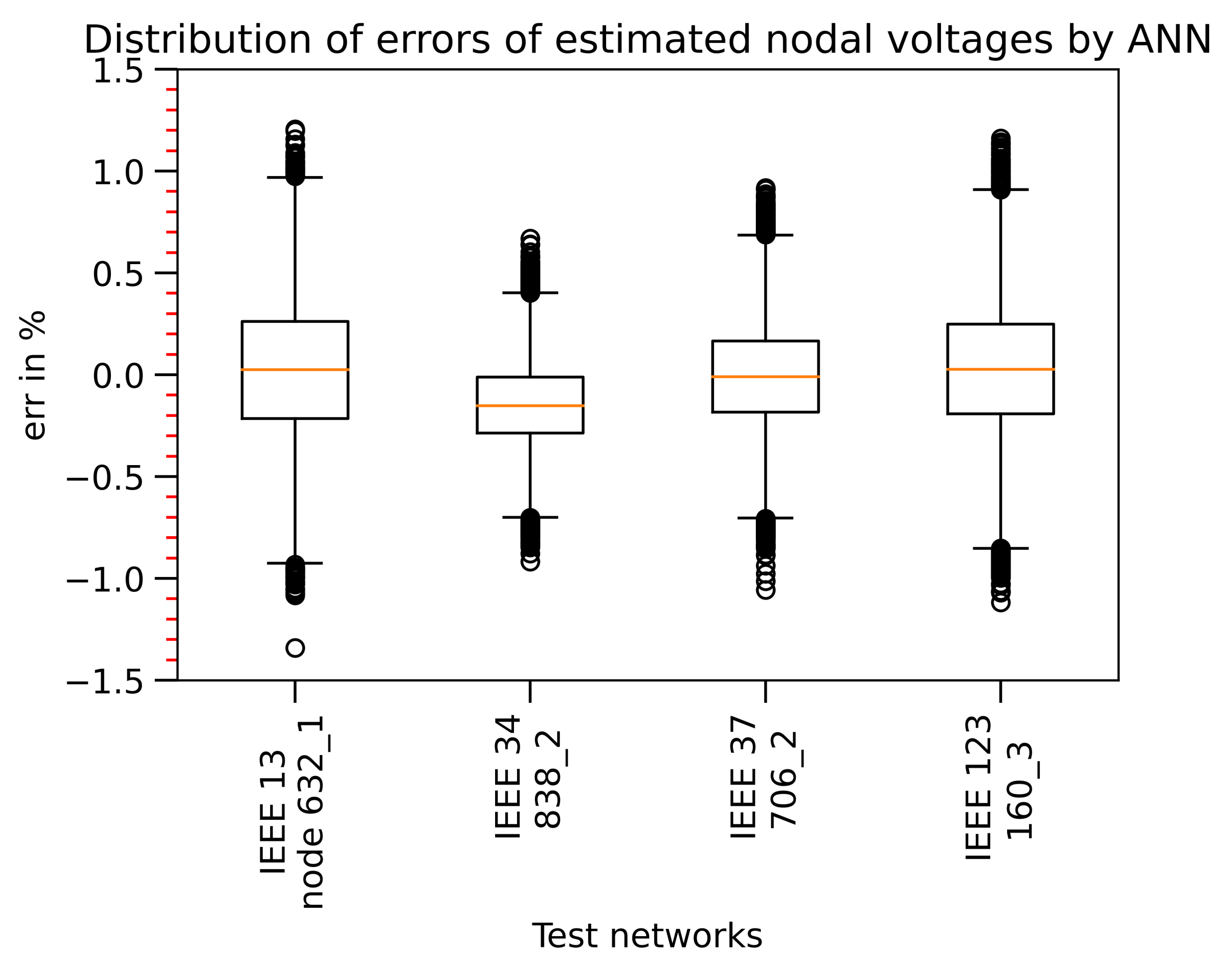
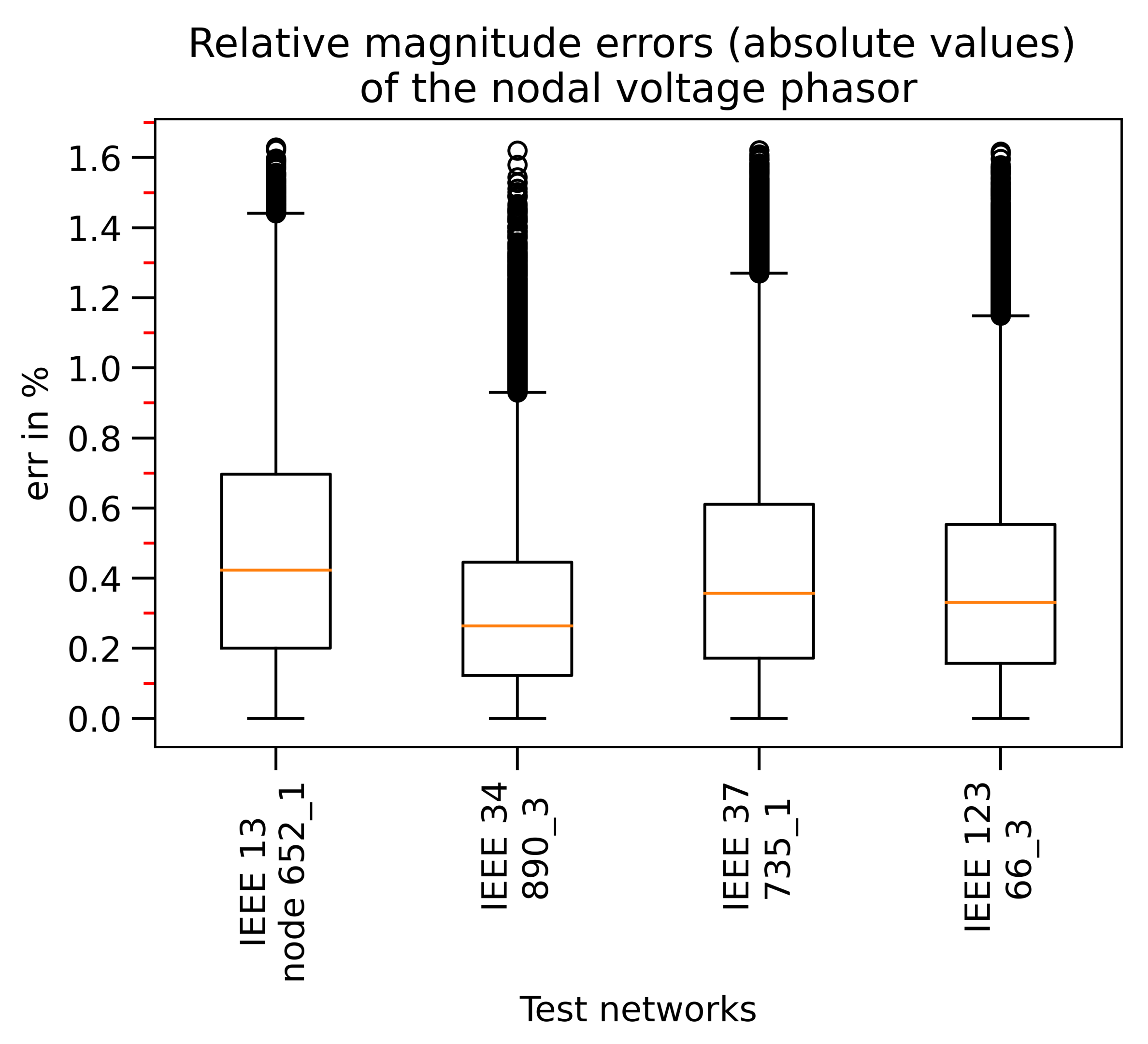
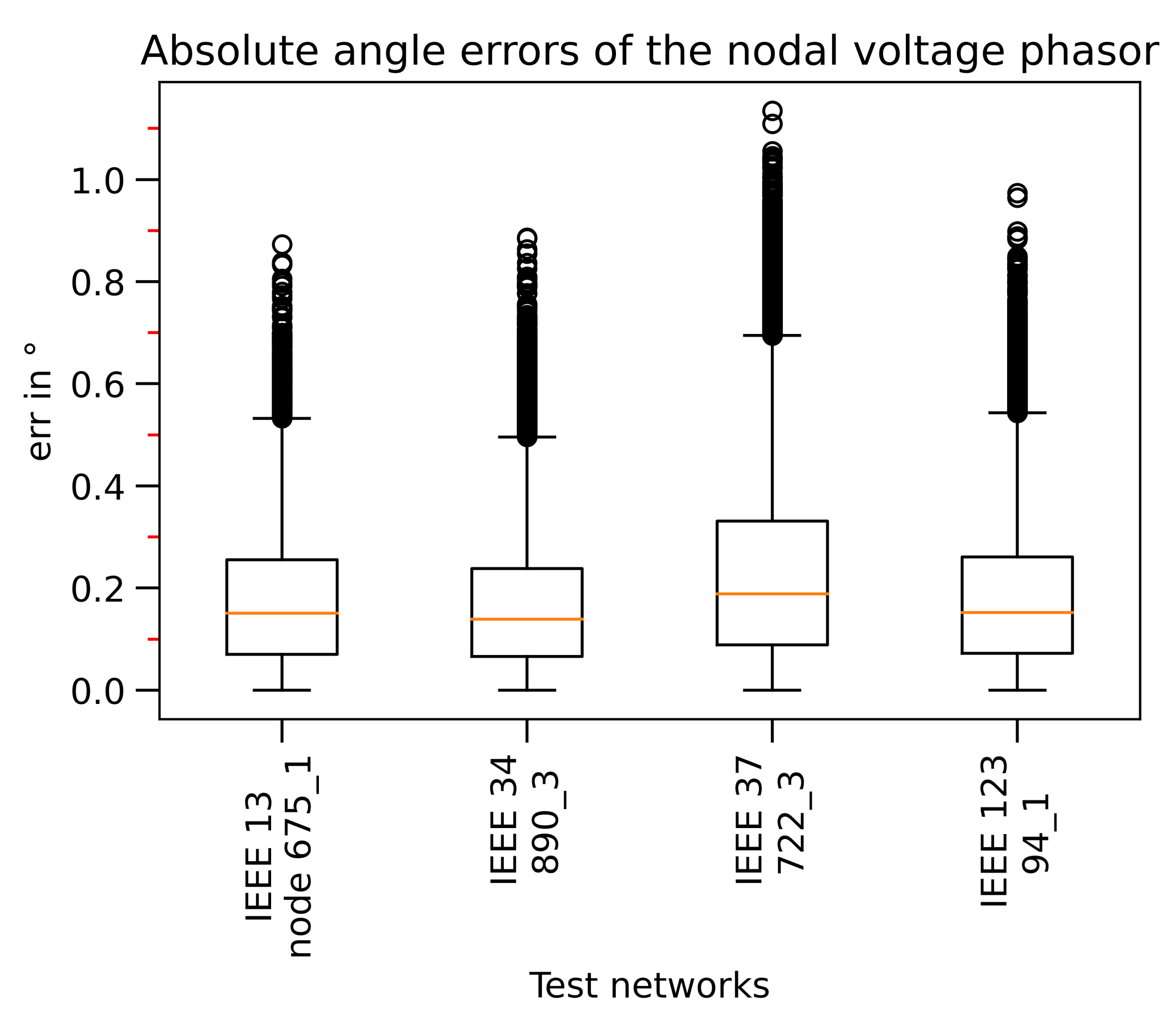
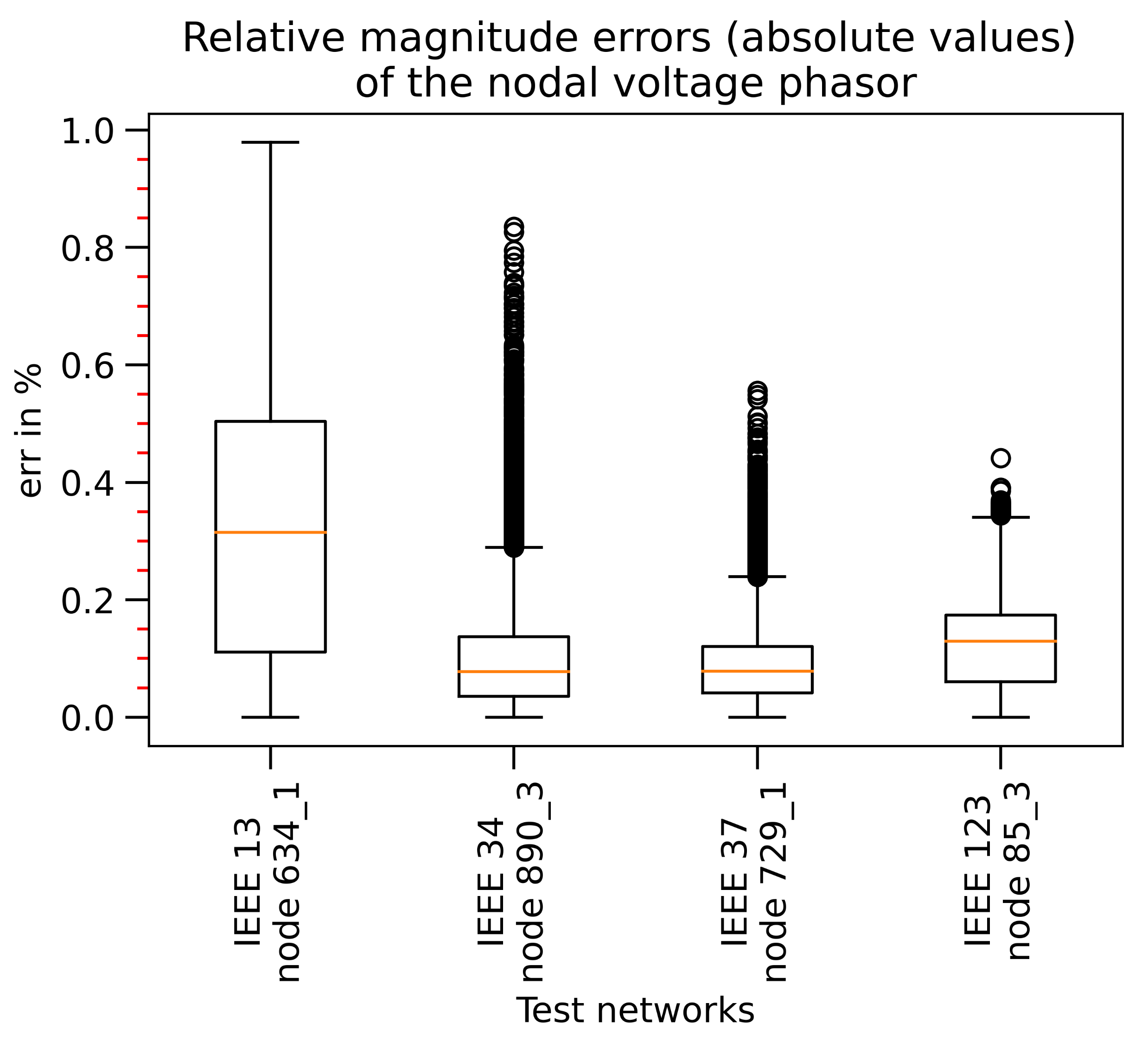
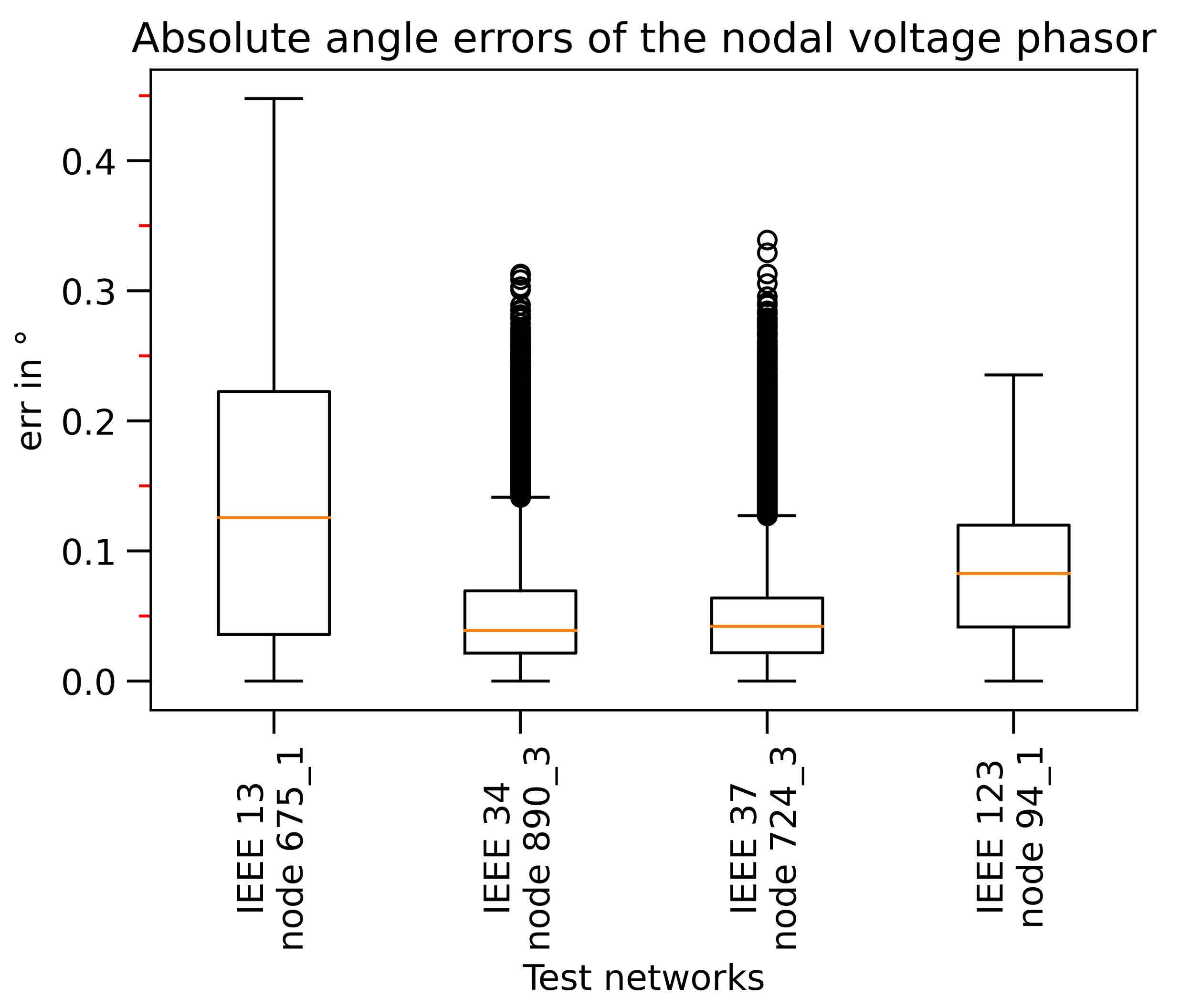
4.1. The Procedure Robustness

Since measurement devices work with some accuracy, robustness of estimation algorithms is usually investigated. Randomly generated errors were added to the real voltage magnitude values to simulate the measurement errors. The errors were generated by using random numbers in the range from −2% to 2% applying the uniform distribution. Usually, in practice, the accuracy of measurement devices is 1% and lower. However, such a high measurement error limit was intentionally set here to investigate the algorithm robustness for a very unfavorable case. The obtained errors were added to the input data for the procedure of Step A2 after which Steps A3 and B2 were performed. It is interesting to compare errors in estimated voltage magnitudes by Steps A3 and B2 for cases with and without considering measurement errors. Without considering the measurement accuracy, the maximal estimation errors of Step A3 (Table 4) are lower than those obtained by Step B2 (Figure 7). The obtained nodal voltage magnitude considering the measurement errors is given in Figure 9 and Figure 10 in the form of box plots showing error distributions. As can be noted, the voltage magnitude estimation by ANN (Step A3) has lower accuracy comparing the estimation not considering measurement errors (comparison of Table 4 and Figure 9). However, Step B1 (the optimization procedure) significantly improves the estimation quality giving slightly higher estimation errors (in Step B2) than in the case when measurement accuracy is considered (comparison of Figure 7 and Figure 10).

In Figure 11, the voltage phasor angles of estimated nodal voltages are presented.

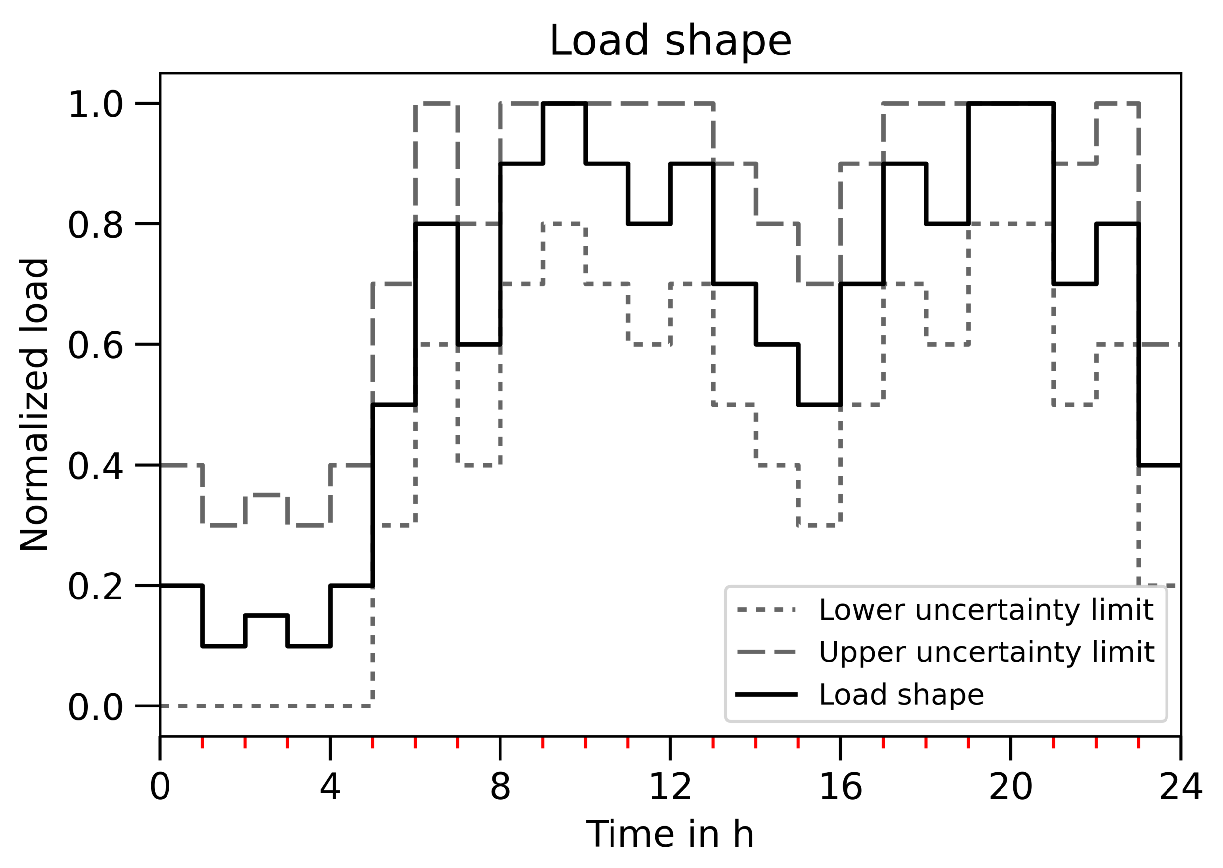
4.2. Scenario Using Consumers’ Load Shape

The consumers’ load shapes are very often known (with more or less uncertainty) in the distribution power network. The load shapes are usually characterized by a consumer type and day/season type. The application of the proposed method was applied to the scenario when the distribution network operator had a load shape of the customers. The load shape, given in Figure 12, was used in the simulations.

In this scenario, the uncertainty in the hourly load values in the range of ±20% was applied and load combinations were generated according to:

$$c_i=rand(-0.2,0.2),P_i=c_i{P}_{i,t},Q_i=c_i{Q}_{i,t},$$

(7)

where $P_{i,t}$ and $Q_{i,t}$ are active and reactive load powers of ith load in hour t. The lower and upper box constraint limits in (6) are defined in the range of the given hourly load $x_t$ with the uncertainty (20% in this case) as:

$$x\in \{x_t-0.2,x_t+0.2\}.$$

(8)

This scenario considers the measurement errors as presented in the previous section. It is important to emphasize that there is no need to repeat the estimation procedure (Stage A, i.e., it is not required to build and train ANN again) before a generated/trained ANN is used. Only a new dataset denoted as Test Data 2 (in Figure 2) was generated according to (7) and Stage B was performed. The highest estimation errors obtained for voltage magnitudes by ANN are in the same ranges as those given in Figure 9 (for generally generated load combinations without applying the load shape).

The results in the box plot related to the estimation error distributions for nodes with the highest error values are presented in Figure 13 and Figure 14 for nodal voltage magnitudes and angles, respectively.

The results in Figure 13 and Figure 14 show that voltage phasor estimation errors are lower when the consumers’ load shapes are known compared to the scenario with the unknown load shape (Figure 10 and Figure 11). The magnitude errors are below 1%, 0.85%, 0.6% and 0.45% of magnitudes and below 0.45${}^{\circ }$, 0.35${}^{\circ }$, 0.35${}^{\circ }$ and 0.25${}^{\circ }$ for voltage angles in the case of tested IEEE 13, 34, 37, and 123 node feeders, respectively. The maximal estimation error in voltage magnitudes and angles, in this case, is lower than the measurement error range and inside the first three quartiles of the simulated data the error is very low (below 0.5%, 0.15%, 0.1% and 0.2% for magnitudes and 0.25${}^{\circ }$, 0.1${}^{\circ }$, 0.1${}^{\circ }$ and 0.15${}^{\circ }$ for angles for IEEE 13, 34, 37 and 123 node test feeders, respectively).

The data (with explanations) used in the simulations are available on: https://drive.google.com/drive/folders/1b4Lx4LJBdNk9vQFBQASMrB3R9HTUeV6i?usp=sharing, accessed on 17 February 2021.

5. Discussion

Based on the presented results, the main features of the proposed method are described here. In the scenario without the measured errors (or with very low errors), Step A3 (ANN) estimates the nodal voltage magnitudes with even lower errors (Figure 5 and Figure 7) than Step B2 (power flow using virtual load values). This is a very interesting outcome because a very simple ANN (with one hidden layer) was used compared to the recent application of a more complex DNN in [5] or MLP ANN with more hidden layers in [6]. The main step that enables using such simple ANN is procedure Step A2, i.e., the procedure step for determining the ANN input and output quantities (Figure 3). However, a more realistic scenario including the measurement errors in the input data shows the requirement for applying procedure Stage B to a more accurate estimation of the voltage magnitudes (high errors for ANN estimation (Figure 9) are significantly decreased by the optimization (Figure 10)) as well as voltage angles. Comparing Figure 7, Figure 8, Figure 10 and Figure 11 leads to the conclusion that the estimation procedure estimates voltage phasors with lower accuracy in the case with measurement errors in comparison to the case without measurement errors. Based on this analysis, it can be stated that the proposed estimation procedure is robust with a low impact of measurement accuracy on it. The additional decreasing of the estimation errors is obtained by using load shapes (but also with a wider range of uncertainty). These improvements in the nodal voltage phasor estimation are caused by defining the narrower decision variable ranges in (8) which is possible by knowing the load shape and its uncertainty. Consequently, the optimization algorithm is directed in the part of the solution space that contains the global optimum solutions and done intensification of the interesting part of the solution space. In other words, the optimization algorithm will find virtual values of the load closer to their real values. Virtual load values will be closer to their real values the narrower is the uncertainty range of the load shape.

The presented results indicate that estimation accuracy depends on the network configuration. The estimation accuracy is comparable to those in the references. In [6], the estimation error of nodal voltage magnitudes (for balanced tested power networks) was below 1% in the case of all load scaled with the same load factor and below 0.43% when time-series input data were e used (this method was not applied to voltage angle estimation). Using the proposed procedure for a more general case (for each load different load factors, highly unbalanced power networks and load shapes with 20% of uncertainty), the voltage phasor magnitude errors were from below 0.5% (IEEE 123) to below 1% (IEEE 13) and the angle errors were from below 0.25${}^{\circ }$ (IEEE 123) to below 0.5${}^{\circ }$ (IEEE 13).

Based on the performed research and presented results, the proposed estimation procedure is as follows:

• The proposed procedure for determining network nodes with and without voltage measurements based on the correlation analysis can keep the required observability level very low (for a more general type of unbalanced power networks).
• Co-simulation and synergy of more computational intelligence methods approach enables estimation of the voltage phasors profile based on very basic measurements and with a limited number of measurements.
• Using the co-simulation setup of different purpose computational tool makes it possible to model the distribution power network more realistically by decreasing the level of assumptions, approximations and neglects in the model.
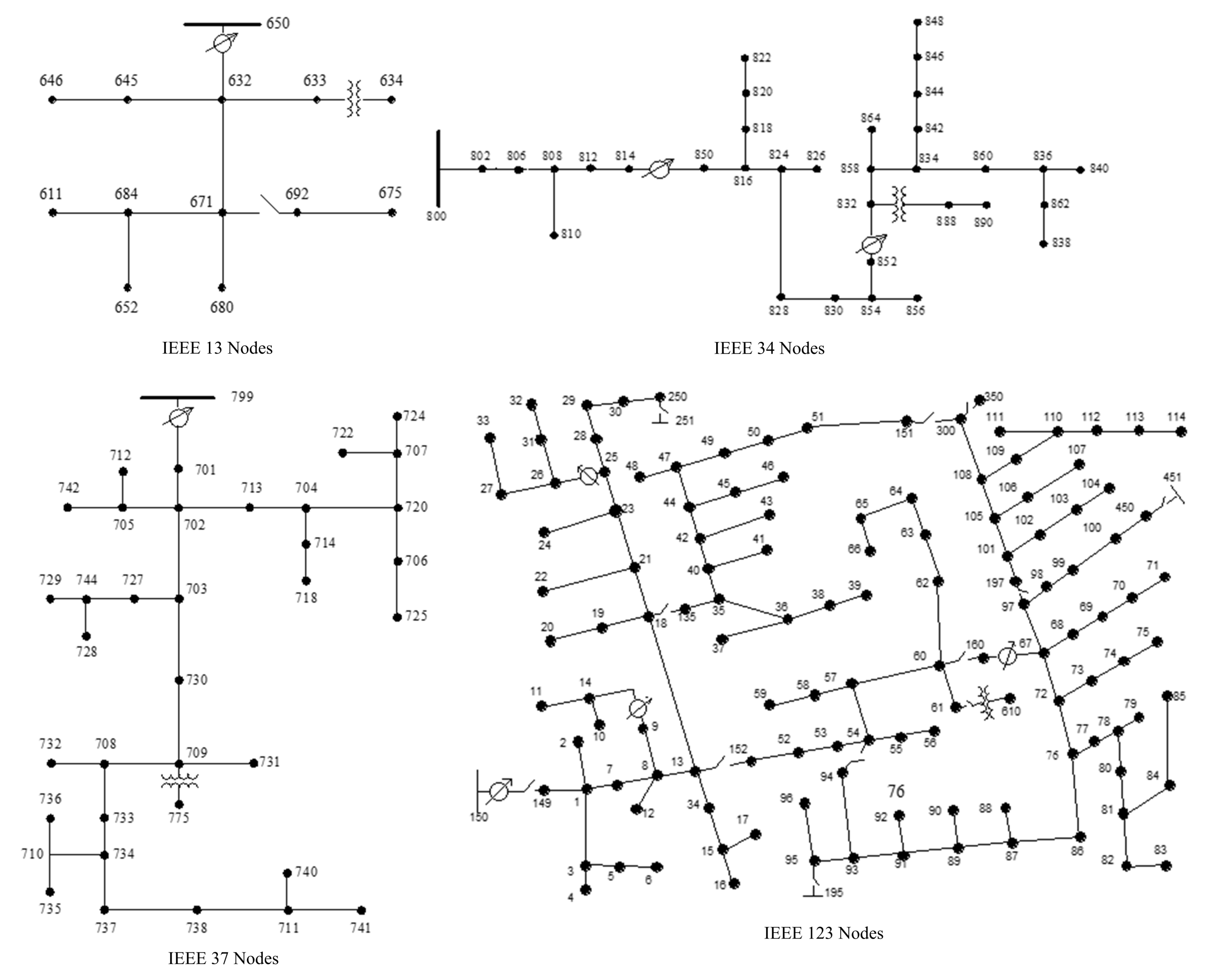
• The required number of nodal voltage magnitude measurements in the proposed method is not highly dependent on the network size. As shown in Table 3, for three networks (IEEE 13, 34 and 37 nodes) with a very different number of nodes, the number of measurements is almost the same. In addition, with a significant increase in the number of network nodes, the number of measurements increased slightly (IEEE 123 nodes).
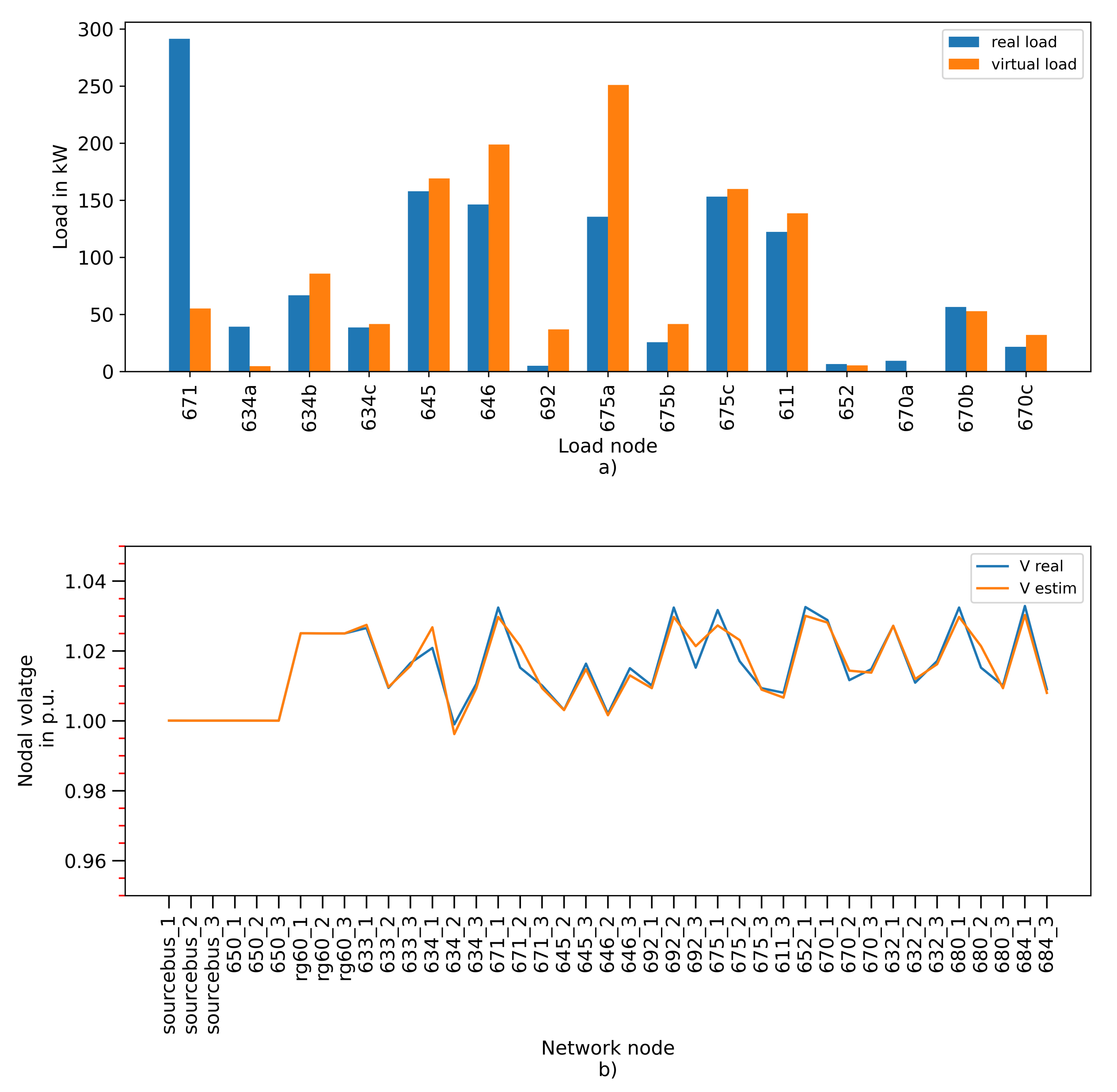
• There are more different load combinations in the network giving very close voltage profiles—this is a very interesting and unexpected conclusion. This conclusion makes it possible to involve the concept of virtual loads. Even though there are significant differences between the values of real and virtual loads, the virtual load concept ensures a quality estimation of the nodal voltage phasor profile.
• Besides achieving the main goal of the nodal voltage phasor estimation, thanks to the physically-based network model and the virtual load concept, other quantities in the network can also be estimated.
• The proposed procedure cannot be applied to the estimation of the real load values in the general case of load changes, i.e., without knowing the consumers’ load shape.

Further research will be directed to investigation procedures for the estimation of real load values to additionally decrease the voltage estimation errors.

6. Conclusions

Based on the presented results, it can be stated that the proposed procedure is able to estimate the nodal voltage phasors with a satisfactory accuracy level by using very limited input data. The applicability of the estimation procedure in the case of decreased measurement data arises from the application of two computational intelligence techniques in synergistic operation. Owing to such an approach, it is possible to estimate the nodal voltage phasors in the distribution network with low observability. Applying the proposed procedure enables the estimation of the nodal voltage phasors with the observability factor in the range from 0.05 to 0.29 depending on the network configuration, lines, loads, etc. It is very interesting to notice that, according to Table 3, the observability factor values are not directly correlated with the network size. The presented framework for the nodal voltage phasor estimation is especially promising in cases with known consumers’ load shapes.

References

1. Al-Wakeel, A.; Wu, J.; Jenkins, N. State estimation of medium voltage distribution networks using smart meter measurements. Appl. Energy 2016, 184, 207–218. [Google Scholar] [CrossRef] [Green Version]
2. Skok, S.; Ivankovic, I.; Cerina, Z. Hybrid State Estimation Model Based on PMU and SCADA Measurements. IFAC-PapersOnLine 2016, 49, 390–394. [Google Scholar] [CrossRef]
3. Manitsas, E.; Singh, R.; Pal, B.C.; Strbac, G. Distribution System State Estimation Using an Artificial Neural Network Approach for Pseudo Measurement Modeling. IEEE Trans. Power Syst. 2012, 27, 1888–1896. [Google Scholar] [CrossRef]
4. Zamzam, A.S.; Fu, X.; Sidiropoulos, N.D. Data-Driven Learning-Based Optimization for Distribution System State Estimation. IEEE Trans. Power Syst. 2019, 34, 4796–4805. [Google Scholar] [CrossRef] [Green Version]
5. Ostrometzky, J.; Berestizshevsky, K.; Bernstein, A.; Zussman, G. Physics-Informed Deep Neural Network Method for Limited Observability State Estimation. arXiv 2019, arXiv:1910.06401. [Google Scholar]
6. Menke, J.H.; Bornhorst, N.; Braun, M. Distribution system monitoring for smart power grids with distributed generation using artificial neural networks. Int. J. Electr. Power Energy Syst. 2019, 113, 472–480. [Google Scholar] [CrossRef] [Green Version]
7. Ashraf, S.M.; Gupta, A.; Choudhary, D.K.; Chakrabarti, S. Voltage stability monitoring of power systems using reduced network and artificial neural network. Int. J. Electr. Power Energy Syst. 2017, 87, 43–51. [Google Scholar] [CrossRef]
8. Soliman Qudaih, Y.; Mitani, Y. Power Distribution System Planning for Smart Grid Applications using ANN. Energy Procedia 2011, 12, 3–9. [Google Scholar] [CrossRef] [Green Version]
9. Aravindhababu, P.; Balamurugan, G. ANN based online voltage estimation. Appl. Soft Comput. 2012, 12, 313–319. [Google Scholar] [CrossRef]
10. Zhou, D.Q.; Annakkage, U.D.; Rajapakse, A.D. Online monitoring of voltage stability margin using an Artificial Neural Network. IEEE Trans. Power Syst. 2010, 25, 1566–1574. [Google Scholar] [CrossRef]
11. Abdel-Nasser, M.; Mahmoud, K.; Kashef, H. A novel smart grid state estimation method based on neural networks. IJIMAI 2018, 5, 92–100. [Google Scholar] [CrossRef] [Green Version]
12. Carcangiu, S.; Fanni, A.; Pegoraro, P.A.; Sias, G.; Sulis, S. Forecasting-Aided Monitoring for the Distribution System State Estimation. Complexity 2020, 2020, 4281219. [Google Scholar] [CrossRef]
13. Majdoub, M.; Boukherouaa, J.; Cheddadi, B.; Belfqih, A.; Sabri, O.; Haidi, T. A Review on Distribution System State Estimation Techniques. In Proceedings of the 2018 6th International Renewable and Sustainable Energy Conference (IRSEC), Rabat, Morocco, 5–8 December 2018; pp. 1–6. [Google Scholar] [CrossRef]
14. Schlüter, M.; Erb, S.O.; Gerdts, M.; Kemble, S.; Rückmann, J.J. MIDACO on MINLP space applications. Adv. Space Res. 2013, 51, 1116–1131. [Google Scholar] [CrossRef]
15. Schlüter, M.; Egea, J.A.; Banga, J.R. Extended ant colony optimization for non-convex mixed integer nonlinear programming. Comput. Oper. Res. 2009, 36, 2217–2229. [Google Scholar] [CrossRef] [Green Version]
16. LeNail, A. NN-SVG: Publication-Ready Neural Network Architecture Schematics. J. Open Source Softw. 2019, 4, 747. [Google Scholar] [CrossRef]
17. Abadi, M.; Agarwal, A.; Barham, P.; Brevdo, E.; Chen, Z.; Citro, C.; Corrado, G.S.; Davis, A.; Dean, J.; Devin, M.; et al. TensorFlow: Large-Scale Machine Learning on Heterogeneous Distributed Systems. 2015. Available online: http://download.tensorflow.org/paper/whitepaper2015.pdf (accessed on 16 May 2019).
18. Chollet, F. Keras. 2015. Available online: https://keras.io/ (accessed on 16 May 2019).
19. Dugan, R.C.; McDermott, T.E. An open source platform for collaborating on smart grid research. In Proceedings of the 2011 IEEE Power and Energy Society General Meeting, Detroit, MI, USA, 24–28 July 2011. [Google Scholar] [CrossRef]
20. Zamee, M.A.; Won, D. Novel Mode Adaptive Artificial Neural Network for Dynamic Learning: Application in Renewable Energy Sources Power Generation Prediction. Energies 2020, 13, 1–29. [Google Scholar] [CrossRef]
21. Corder, G.W.; Foreman, D.I. Nonparametric Statistics for Non-Statisticians; John Wiley & Sons, Inc.: Hoboken, NJ, USA, 2009. [Google Scholar] [CrossRef]
22. Kendall, M.; Gibbons, J. Rank Correlation Methods; Edward Arnold: New York, NY, USA, 1990; pp. 1–260. [Google Scholar]
23. Distribution Test Feeder Working Group—IEEE PES Distribution System Analysis Subcommittee. Distribution Test Feeders. Available online: https://ewh.ieee.org/soc/pes/dsacom/testfeeders/ (accessed on 15 May 2018).
Figure 1. Multi-layer perceptron ANN with one hidden layer (the figure is generated using an online tool [16]).
Electronics 10 00522 g001
Figure 2. The workflow of the proposed framework for the voltage phasor profile estimation.
Electronics 10 00522 g002
Figure 3. The procedure for determining the number of ANN inputs and outputs—Step A2 in a closed loop with Step A3.
Electronics 10 00522 g003
Figure 4. Configuration of test distribution feeders according to Distribution Test Feeder Working Group - IEEE PES Distribution System Analysis Subcommittee [23].
Electronics 10 00522 g004
Figure 5. Box plot of the error distributions in the network nodes for the tested systems (nodal voltage magnitudes estimated by Step A3).
Electronics 10 00522 g005
Figure 6. (a) Different load combinations resulting in (b) close voltage profiles. Example for IEEE 13 node test feeder.
Electronics 10 00522 g006
Figure 7. Distribution of relative errors of nodal voltage phasor magnitudes for nodes with the highest errors.
Electronics 10 00522 g007
Figure 8. Distribution of absolute errors of nodal voltage phasor angles for nodes with the highest errors.
Electronics 10 00522 g008
Figure 9. Distribution of percentage errors (absolute amounts) of nodal voltage phasor magnitudes for nodes with the highest errors obtained in Step A3.
Electronics 10 00522 g009
Figure 10. Distribution of percentage errors (absolute amounts) of nodal voltage phasor magnitudes for nodes with the highest errors obtained in Step B2.
Electronics 10 00522 g010
Figure 11. Distribution of absolute errors of nodal voltage phasor angles for nodes with the highest errors.
Electronics 10 00522 g011
Figure 12. Consumers’ load shapes with the uncertainty range of 20%.
Electronics 10 00522 g012
Figure 13. Distribution of absolute errors of nodal voltage phasor magnitudes for nodes with the highest errors (scenario considering the load shape).
Electronics 10 00522 g013
Figure 14. Distribution of absolute errors of nodal voltage phasor angles for nodes with the highest errors (scenario considering the load shape).
Electronics 10 00522 g014