
Improving Performance Estimation for Design Space Exploration for Convolutional Neural Network Accelerators †

Abstract
:1. Introduction
2. Background and Related Work
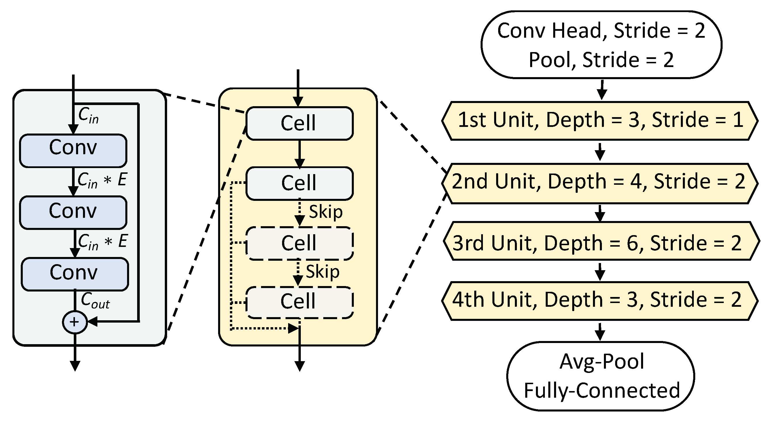
2.1. Neural Networks
| Algorithm 1: Convolution. |
| Input: Input feature map of shape ; weight matrix of shape Output: Output feature map of shape
|
2.2. Performance Estimation
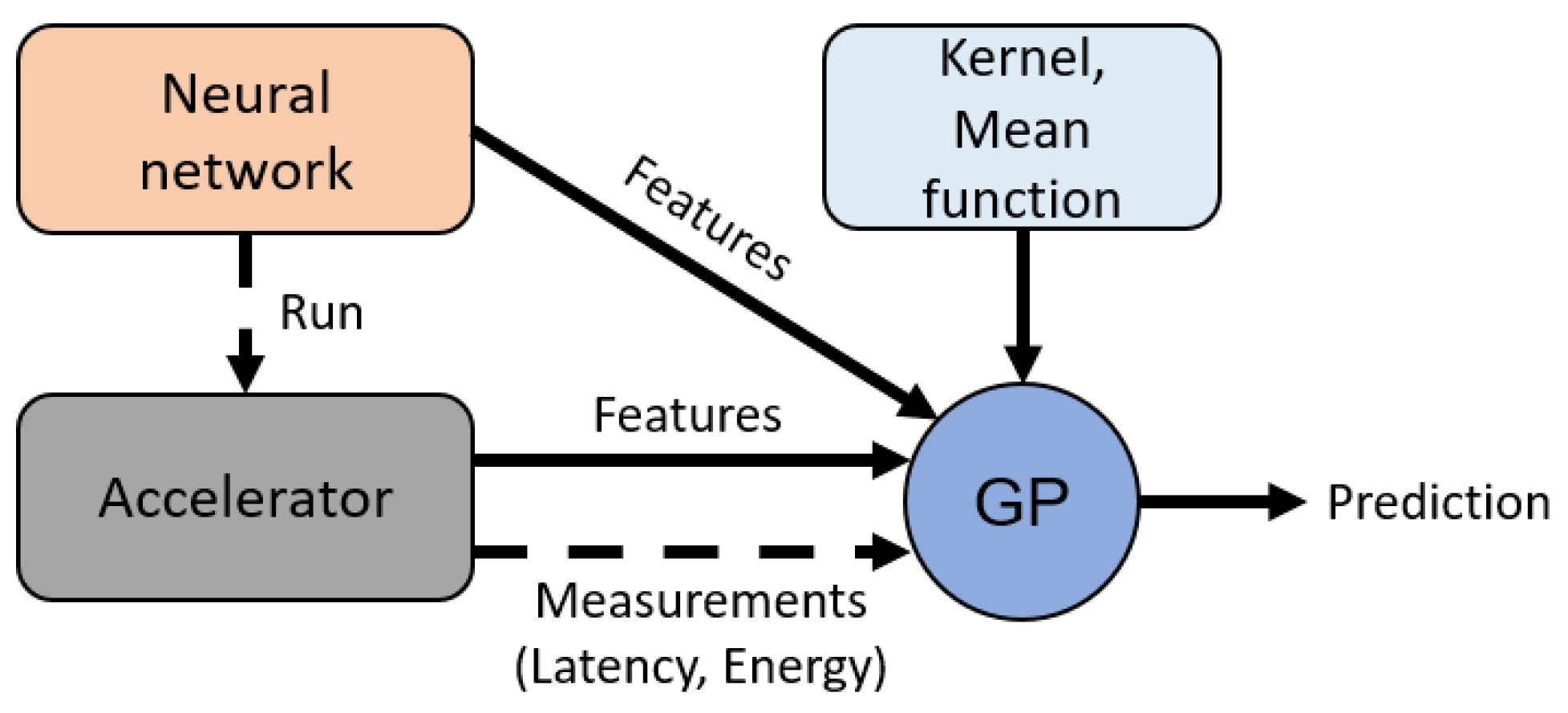
3. Method
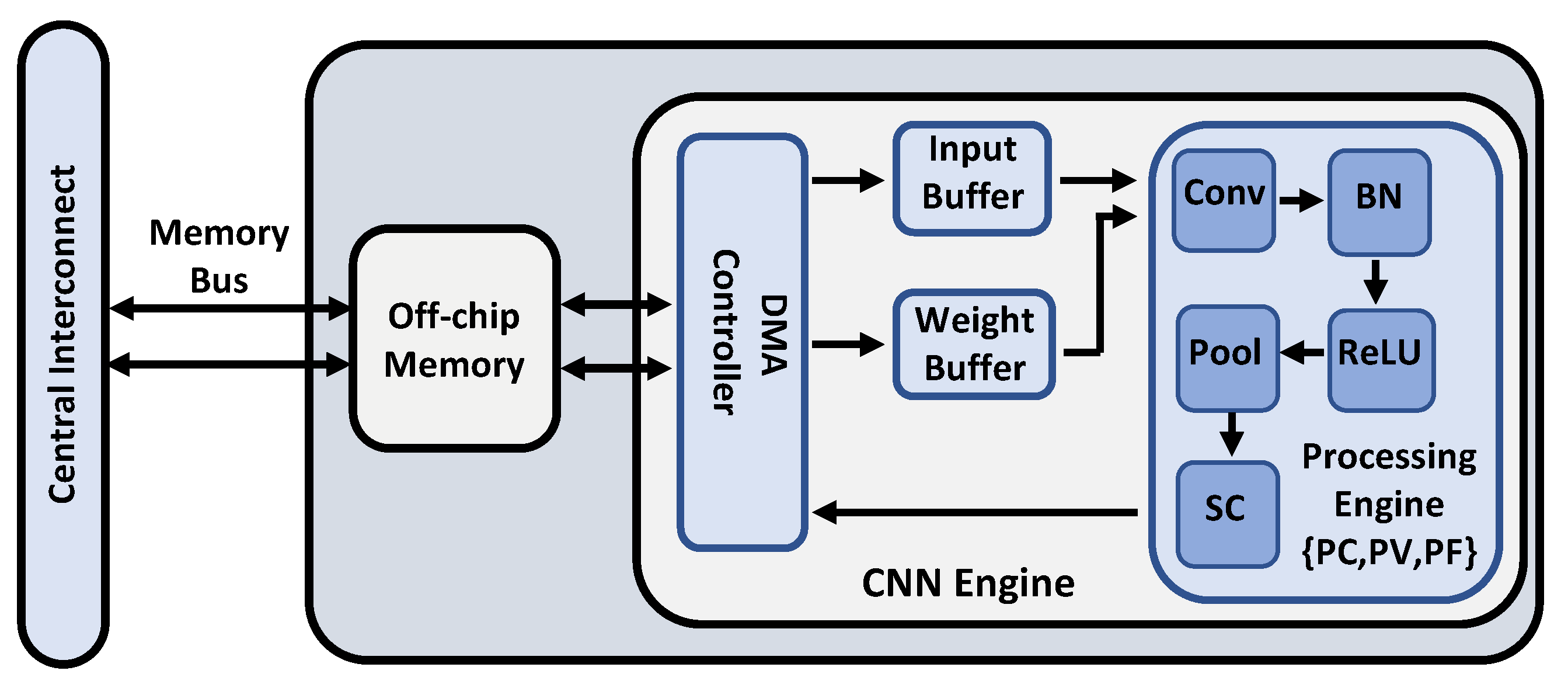
4. Hardware Design
4.1. Accelerator’s Architecture
| Algorithm 2: Channel-major computational pattern. |
| Input: Input feature map of shape ; weight matrix of shape Output: Output feature map of shape
|
4.2. Standard Analytical Latency Model
- Loading time, i.e., the time to load the input into the on-chip memory. Note that the loading of the data is in parallel with respect to the channel parallelism :
- Computation time, i.e., the time to compute parallel filters and channels, respectively:
- Storing time, i.e., the time to store the output back to the off-chip memory. Note that similar to the input loading time, the storage time is divided by the channel parallelism :
5. Experiments
5.1. Evaluation for FPGA Design
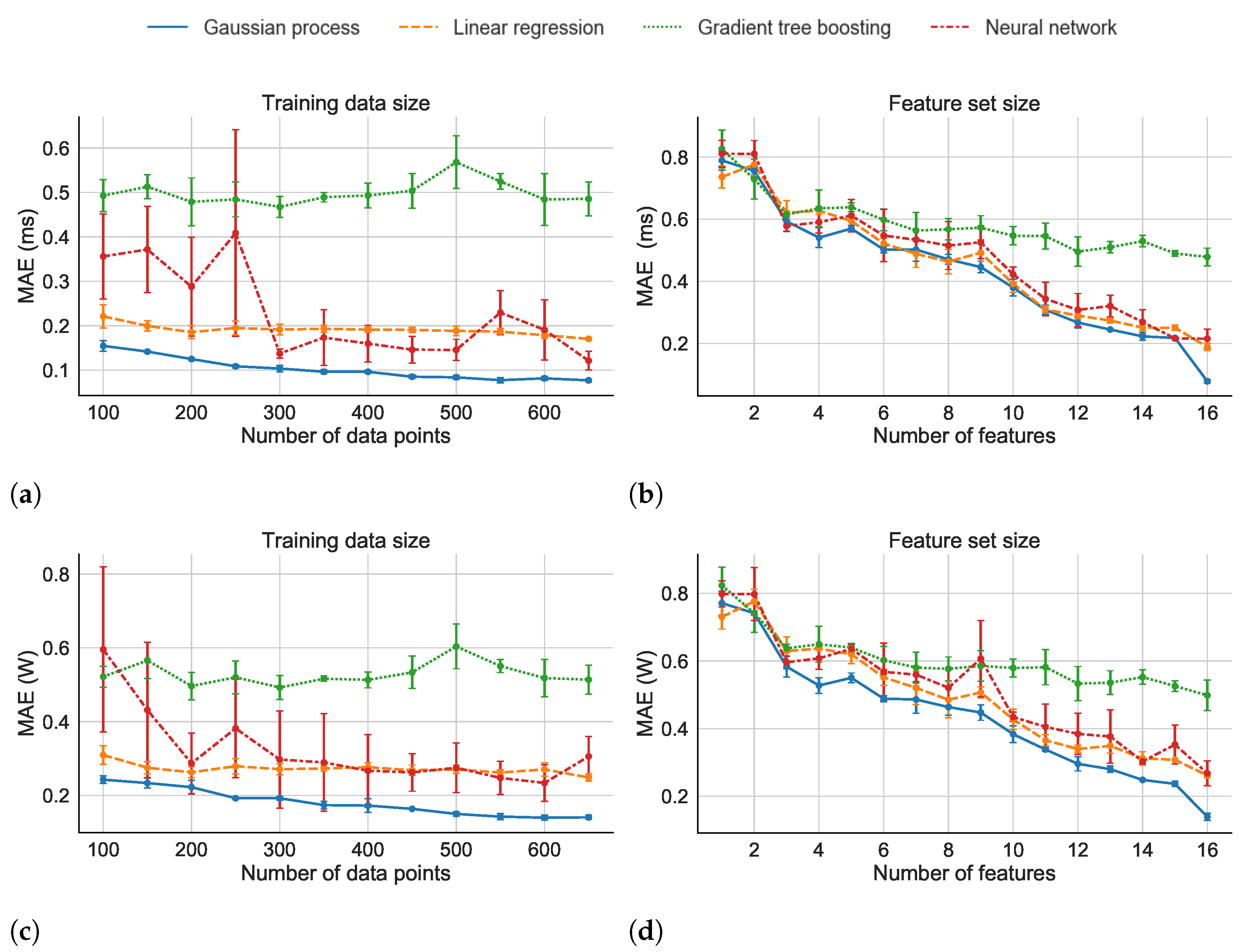
5.2. Evaluation on the ASIC Design
6. Conclusions
Author Contributions
Funding
Data Availability Statement
Acknowledgments
Conflicts of Interest
Abbreviations
| ASIC | Application-specific integrated circuit |
| CPU | Central processing unit |
| CNN | Convolutional neural network |
| DSE | Design space exploration |
| FPGA | Field-programmable gate array |
| GP | Gaussian process |
| GPU | Graphical processing unit |
| GTB | Gradient tree boosting |
| LOOCV | Leave-one-out cross-validation |
| LR | Linear regression |
| MAE | Mean absolute error |
| NN | Neural network |
References
- Ferianc, M.; Fan, H.; Rodrigues, M. VINNAS: Variational Inference based Neural Network Architecture Search. arXiv 2020, arXiv:2007.06103. [Google Scholar]
- Fan, H.; Liu, S.; Ferianc, M.; Ng, H.C.; Que, Z.; Liu, S.; Niu, X.; Luk, W. A Real-Time Object Detection Accelerator with Compressed SSDLite on FPGA. In Proceedings of the 2018 International Conference on Field-Programmable Technology (FPT), Naha Okinawa, Japan, 11–15 December 2018; pp. 14–21. [Google Scholar]
- Liu, S.; Luk, W. Towards an Efficient Accelerator for DNN-Based Remote Sensing Image Segmentation on FPGAs. In Proceedings of the 2019 29th International Conference on Field Programmable Logic and Applications (FPL), Barcelona, Spain, 8–12 September 2019; pp. 187–193. [Google Scholar]
- Brown, T.B.; Mann, B.; Ryder, N.; Subbiah, M.; Kaplan, J.; Dhariwal, P.; Neelakantan, A.; Shyam, P.; Sastry, G.; Askell, A.; et al. Language models are few-shot learners. arXiv 2020, arXiv:2005.14165. [Google Scholar]
- Kwon, Y.; Won, J.H.; Kim, B.J.; Paik, M.C. Uncertainty quantification using Bayesian neural networks in classification: Application to biomedical image segmentation. Comput. Stat. Data Anal. 2020, 142, 106816. [Google Scholar] [CrossRef]
- McAllister, R.; Gal, Y.; Kendall, A.; Van Der Wilk, M.; Shah, A.; Cipolla, R.; Weller, A. Concrete Problems for Autonomous Vehicle Safety: Advantages of Bayesian Deep Learning. In Proceedings of the 26th International Joint Conference on Artificial Intelligence (IJCAI’17), Buenos Aires, Argentina, 25–31 July 2017; pp. 4745–4753. [Google Scholar]
- Xuan-Mung, N.; Hong, S.K. Barometric altitude measurement fault diagnosis for the improvement of quadcopter altitude control. In Proceedings of the 2019 19th International Conference on Control, Automation and Systems (ICCAS), Jeju, Korea, 15–18 October 2019; pp. 1359–1364. [Google Scholar]
- Park, D.; Yu, H.; Xuan-Mung, N.; Lee, J.; Hong, S.K. Multicopter PID Attitude Controller Gain Auto-tuning through Reinforcement Learning Neural Networks. In Proceedings of the 2019 2nd International Conference on Control and Robot Technology, Phuket, Thailand, 25–27 October 2019; pp. 80–84. [Google Scholar]
- Nguyen, N.P.; Mung, N.X.; Thanh Ha, L.N.N.; Huynh, T.T.; Hong, S.K. Finite-Time Attitude Fault Tolerant Control of Quadcopter System via Neural Networks. Mathematics 2020, 8, 1541. [Google Scholar] [CrossRef]
- Mittal, S. A survey of FPGA based accelerators for convolutional neural networks. Neural Comput. Appl. 2020, 32, 1109–1139. [Google Scholar] [CrossRef]
- Rahman, A.; Oh, S.; Lee, J.; Choi, K. Design space exploration of FPGA accelerators for convolutional neural networks. In Proceedings of the Design, Automation & Test in Europe Conference & Exhibition (DATE), Lausanne, Switzerland, 27–31 March 2017; pp. 1147–1152. [Google Scholar]
- Yasudo, R.; Coutinho, J.; Varbanescu, A.; Luk, W.; Amano, H.; Becker, T. Performance Estimation for Exascale Reconfigurable Dataflow Platforms. In Proceedings of the 2018 International Conference on Field-Programmable Technology (FPT), Naha Okinawa, Japan, 11–15 December 2018; pp. 314–317. [Google Scholar]
- Dai, S.; Zhou, Y.; Zhang, H.; Ustun, E.; Young, E.F.; Zhang, Z. Fast and accurate estimation of quality of results in high-level synthesis with machine learning. In Proceedings of the 2018 IEEE 26th Annual International Symposium on Field-Programmable Custom Computing Machines (FCCM), Boulder, CO, USA, 29 April–1 May 2018; pp. 129–132. [Google Scholar]
- Liu, S.; Fan, H.; Niu, X.; Ng, H.C.; Chu, Y.; Luk, W. Optimizing CNN based Segmentation with Deeply Customized Convolutional and Deconvolutional Architectures on FPGA. ACM Trans. Reconfig. Technol. Syst. 2018, 11, 1–22. [Google Scholar] [CrossRef]
- Williams, C.K.; Rasmussen, C.E. Gaussian processes for regression. Adv. Neural Inf. Process. Syst. 1996, 8, 514–520. [Google Scholar]
- Ferianc, M.; Fan, H.; Chu, R.S.; Stano, J.; Luk, W. Improving Performance Estimation for FPGA-Based Accelerators for Convolutional Neural Networks. In International Symposium on Applied Reconfigurable Computing; Springer: Berlin, Germany, 2020; pp. 3–13. [Google Scholar]
- He, K.; Zhang, X.; Ren, S.; Sun, J. Deep Residual Learning for Image Recognition. In Proceedings of the 2016 IEEE Conference on Computer Vision and Pattern Recognition (CVPR), Las Vegas, NV, USA, 27–30 June 2016; Volume 2016, pp. 770–778. [Google Scholar]
- Liu, W.; Anguelov, D.; Erhan, D.; Szegedy, C.; Reed, S.; Fu, C.Y.; Berg, A. SSD: Single shot multibox detector. In Lecture Notes in Computer Science (Including Subseries Lecture Notes in Artificial Intelligence and Lecture Notes in Bioinformatics); Springer: Berlin, Germany, 2016; Volume 9905, pp. 21–37. [Google Scholar]
- Redmon, J.; Divvala, S.; Girshick, R.; Farhadi, A. You Only Look Once: Unified, Real-Time Object Detection. In Proceedings of the 2016 IEEE Conference on Computer Vision and Pattern Recognition (CVPR), Las Vegas, NV, USA, 27–30 June 2016; Volume 3, pp. 779–788. [Google Scholar]
- LeCun, Y.; Boser, B.; Denker, J.S.; Henderson, D.; Howard, R.E.; Hubbard, W.; Jackel, L.D. Backpropagation applied to handwritten zip code recognition. Neural Comput. 1989, 1, 541–551. [Google Scholar] [CrossRef]
- Fan, H.; Luo, C.; Zeng, C.; Ferianc, M.; Que, Z.; Liu, S.; Niu, X.; Luk, W. F-E3D: FPGA based Acceleration of an Efficient 3D Convolutional Neural Network for Human Action Recognition. In Proceedings of the 2019 IEEE 30th International Conference on Application-specific Systems, Architectures and Processors (ASAP), New York, NY, USA, 15–17 July 2019; Volume 2160, pp. 1–8. [Google Scholar]
- Venieris, S.; Kouris, A.; Bouganis, C.S. Toolflows for Mapping Convolutional Neural Networks on FPGAs: A Survey and Future Directions; ACM: New York, NY, USA, 2018; Volume 51, pp. 1–39. [Google Scholar]
- Rasmussen, C.E. Gaussian Processes in Machine Learning; The MIT Press: Cambridge, MA, USA, 2005. [Google Scholar]
- Ioffe, S.; Szegedy, C. Batch normalization: Accelerating deep network training by reducing internal covariate shift. arXiv 2015, arXiv:1502.03167. [Google Scholar]
- Jacob, B.; Kligys, S.; Chen, B.; Zhu, M.; Tang, M.; Howard, A.; Adam, H.; Kalenichenko, D. Quantization and training of neural networks for efficient integer-arithmetic-only inference. In Proceedings of the IEEE Conference on Computer Vision and Pattern Recognition, Salt Lake City, UT, USA, 18–23 June 2018; pp. 2704–2713. [Google Scholar]
- Pedregosa, F.; Varoquaux, G.; Gramfort, A.; Michel, V.; Thirion, B.; Grisel, O.; Blondel, M.; Prettenhofer, P.; Weiss, R.; Dubourg, V.; et al. Scikit-learn: Machine Learning in Python. J. Mach. Learn. Res. 2011, 12, 2825–2830. [Google Scholar]
- Friedman, J.H. Stochastic gradient boosting. In Computational Statistics & Data Analysis; Elsevier: Amsterdam, The Netherlands, 2002; Volume 38, pp. 367–378. [Google Scholar]
- Abadi, M.; Agarwal, A.; Barham, P.; Brevdo, E.; Chen, Z.; Citro, C.; Davis, A.; Dean, J.; Devin, M.; Ghemawat, S.; et al. TensorFlow: Large-Scale Machine Learning on Heterogeneous Systems. 2015. Available online: https://www.tensorflow.org/ (accessed on 14 December 2020).
- Kingma, D.P.; Ba, J. Adam: A method for stochastic optimization. arXiv 2014, arXiv:1412.6980. [Google Scholar]
- Matthews, D.G.; Alexander, G.; Van Der Wilk, M.; Nickson, T.; Fujii, K.; Boukouvalas, A.; León-Villagrá, P.; Ghahramani, Z.; Hensman, J. GPflow: A Gaussian process library using TensorFlow. J. Mach. Learn. Res. 2017, 18, 1299–1304. [Google Scholar]
- Intel Corporation. eASIC Technology. 2018. Available online: https://www.intel.co.uk/content/www/uk/en/products/programmable/asic/easic-devices.html (accessed on 2 December 2020).
- Venieris, S.I.; Bouganis, C.S. fpgaConvNet: A framework for mapping convolutional neural networks on FPGAs. In Proceedings of the 2016 IEEE 24th Annual International Symposium on Field-Programmable Custom Computing Machines (FCCM), Washington, DC, USA, 1–3 May 2016; pp. 40–47. [Google Scholar]
- Simonyan, K.; Zisserman, A. Very deep convolutional networks for large-scale image recognition. arXiv 2014, arXiv:1409.1556. [Google Scholar]
- Titsias, M. Variational learning of inducing variables in sparse Gaussian processes. In Proceedings of the Twelfth International Conference on Artificial Intelligence and Statistics (AISTATS), Clearwater Beach, FL, USA, 16–18 April 2009; pp. 567–574. [Google Scholar]


| Height of the input feature map | Width of the input feature map | ||
| Height of the output feature map | Width of the output feature map | ||
| K | Kernel size | F | Number of filters |
| C | Number of channels | s | Stride in a convolution |
| W | Weights in a neural network | Parallelism in the filter dimension | |
| Parallelism in the channel dimension | Parallelism in the data vector dimension | ||
| (MHz) | Memory access clock cycle time | (MHz) | Logic clock cycle time |
| (%) | Memory transfer efficiency | S (bits) | Memory transfer size |
| (bits) | Processing data width | M | Number of input features |
| B | Number of layers in a neural network | N | Number of training samples |
| Sizes | Number of Operations/Data Size |
|---|---|
| Number of compute operations | |
| Input size | |
| Weights size | |
| Output size |
| Parameter | Min | Mean | Max |
|---|---|---|---|
| 1 | 42 | 418 | |
| 1 | 37 | 416 | |
| K | 1 | 2 | 7 |
| C | 3 | 360 | 2048 |
| F | 64 | 371 | 2048 |
| Latency (ms) | 0.018 | 0.841 | 11.727 |
| Methods | Layer-Wise Latency LOOCV MAE (ms) | Implementation and Optimiser | Properties |
|---|---|---|---|
| Standard method | 0.450 | None | None |
| Linear regression | 0.450 | Sklearn [26] | Default |
| Gradient tree boosting | 0.607 | Sklearn [26]; AdaBoost [27] | Learning rate: 0.1 Number of trees: 10 Maximum depth: 3 |
| Neural network | 1.257 | TensorFlow [28]; Adam [29] | Batch size: 8 Learning rate: 0.1 Regulariser: L2, 0.001 Number of nodes: 10,10,1 Activations: ReLU |
| Our method | 0.312 | GPFlow [30]; Adam [29] | Mean function: Learning rate: 0.001 Kernel: Matérn 3/2 |
| SSD | ResNet-50 | Yolo | VGG-16 [33] | |||||
|---|---|---|---|---|---|---|---|---|
| Latency | FPS/W | Latency | FPS/W | Latency | FPS/W | Latency | FPS/W | |
| (ms) | (ms) | (ms) | (ms) | |||||
| FPGA | 3.24 | 7.01 | 4.62 | 4.92 | 41.22 | 0.55 | 23.18 | 0.98 |
| eASIC | 2.39 | 22.02 | 3.06 | 17.20 | 31.55 | 1.67 | 15.35 | 3.43 |
| Methods | Latency | Energy | Implementation | Properties |
|---|---|---|---|---|
| MAE (ms) | MAE (W) | and Optimiser | ||
| Linear regression | 0.177 | 0.272 | Sklearn [26] | Default |
| Gradient tree boosting | 0.476 | 0.501 | Sklearn [26]; AdaBoost [27] | Learning rate: 0.1 Number of trees: 10 Maximum depth: 3 |
| Neural network | 0.108 | 0.241 | TensorFlow [28]; Adam [29] | Batch size: 8 Learning rate: 0.1 Regulariser: L2, 0.001 Number of nodes: 10,10,1 Activations: ReLU |
| Our method | 0.079 | 0.151 | GPFlow [30]; Adam [29] | Mean function: 0 Learning rate: 0.001 Kernel: Matérn 3/2 |
Publisher’s Note: MDPI stays neutral with regard to jurisdictional claims in published maps and institutional affiliations. |
© 2021 by the authors. Licensee MDPI, Basel, Switzerland. This article is an open access article distributed under the terms and conditions of the Creative Commons Attribution (CC BY) license (http://creativecommons.org/licenses/by/4.0/).
Share and Cite
Ferianc, M.; Fan, H.; Manocha, D.; Zhou, H.; Liu, S.; Niu, X.; Luk, W. Improving Performance Estimation for Design Space Exploration for Convolutional Neural Network Accelerators. Electronics 2021, 10, 520. https://doi.org/10.3390/electronics10040520
Ferianc M, Fan H, Manocha D, Zhou H, Liu S, Niu X, Luk W. Improving Performance Estimation for Design Space Exploration for Convolutional Neural Network Accelerators. Electronics. 2021; 10(4):520. https://doi.org/10.3390/electronics10040520
Chicago/Turabian StyleFerianc, Martin, Hongxiang Fan, Divyansh Manocha, Hongyu Zhou, Shuanglong Liu, Xinyu Niu, and Wayne Luk. 2021. "Improving Performance Estimation for Design Space Exploration for Convolutional Neural Network Accelerators" Electronics 10, no. 4: 520. https://doi.org/10.3390/electronics10040520