
An Efficient FPGA Implementation of Richardson-Lucy Deconvolution Algorithm for Hyperspectral Images


Abstract
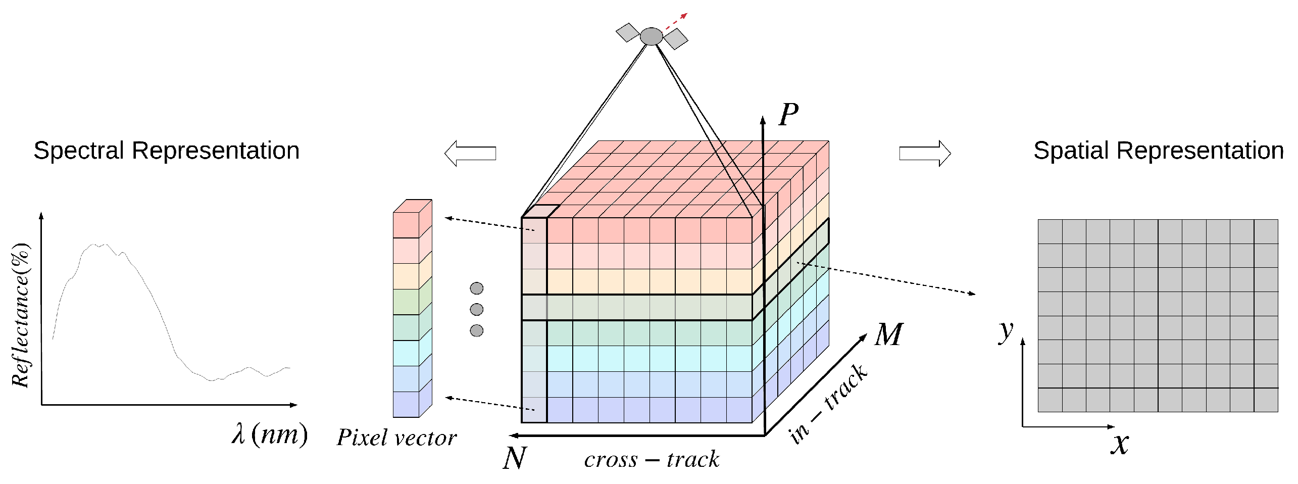
:1. Introduction
2. Background
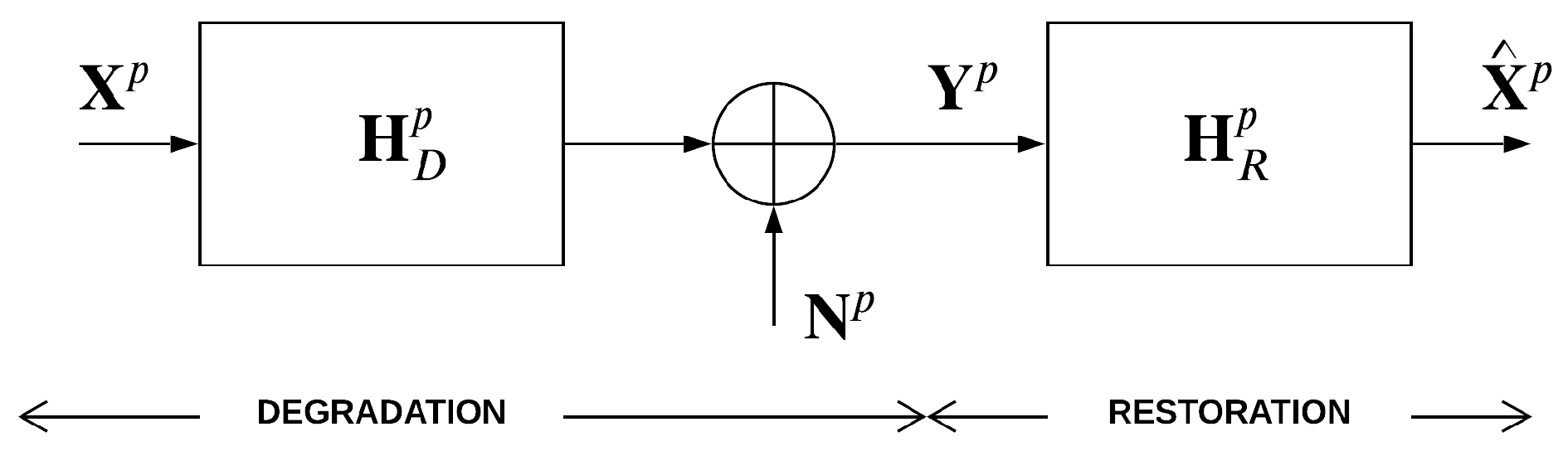
2.1. Image Degradation
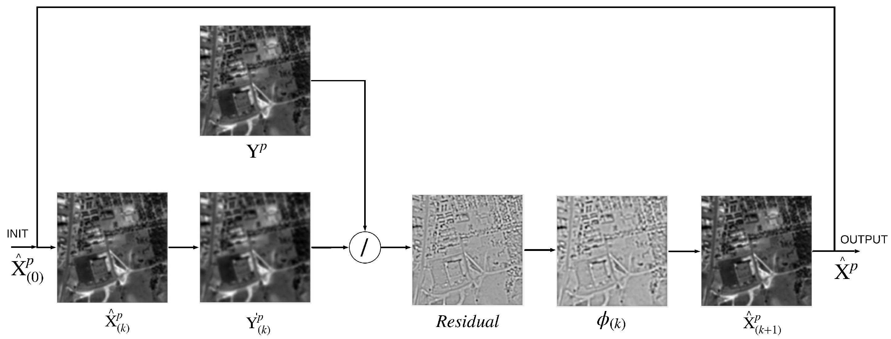
2.2. Image Restoration
- decision on an initial estimate, ;
- computation of the residual, ;
- computation of the correction factor, ; and
- update of the initial estimate, .
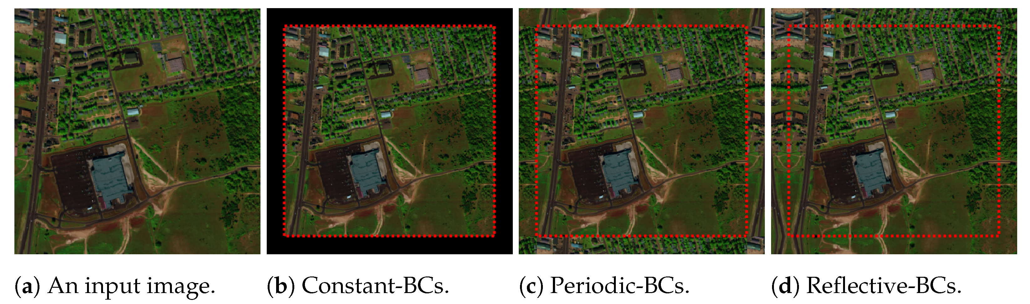
2.3. Border Handling
2.4. Image Quality Assessment
3. RL Deconvolution Algorithm Analysis
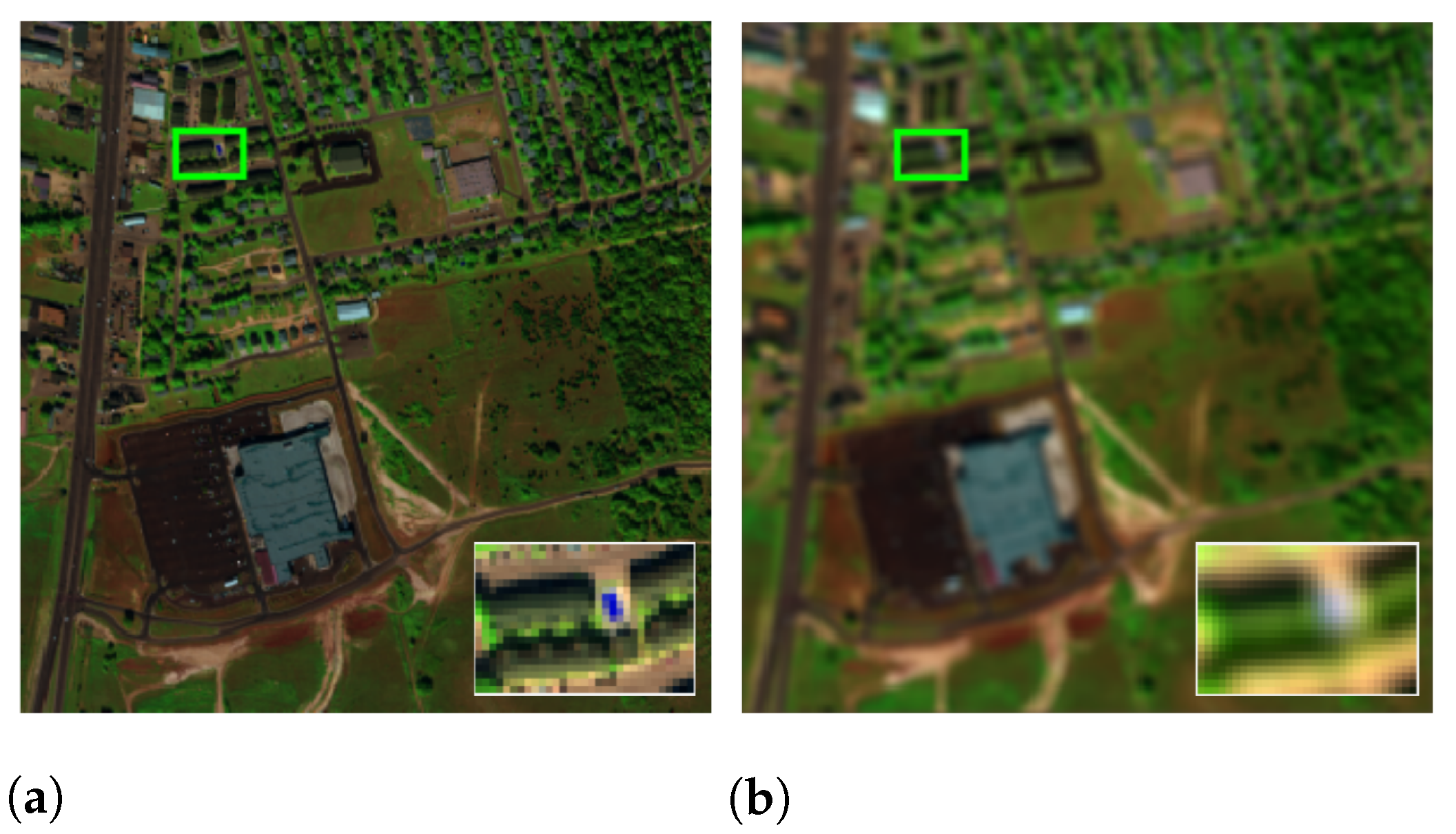
3.1. Hyperspectral Data Set
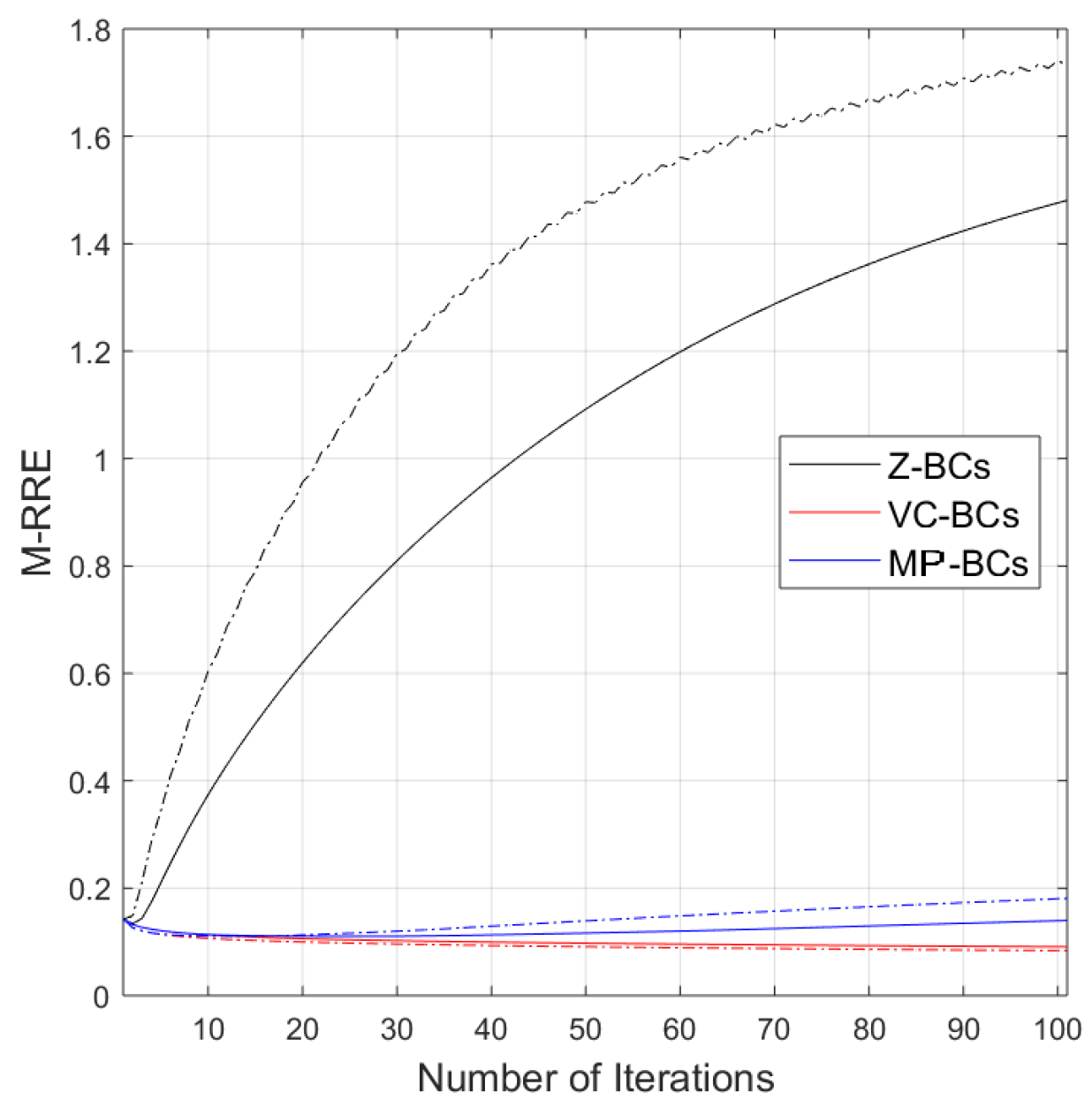
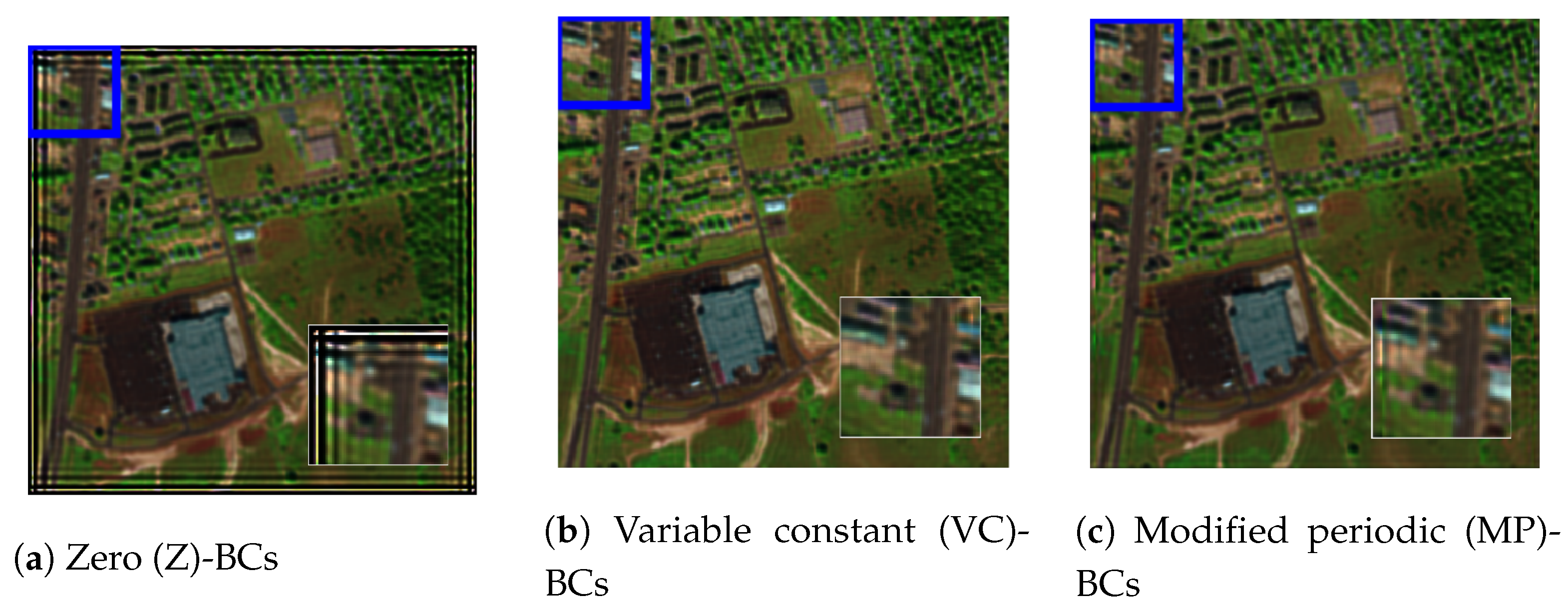
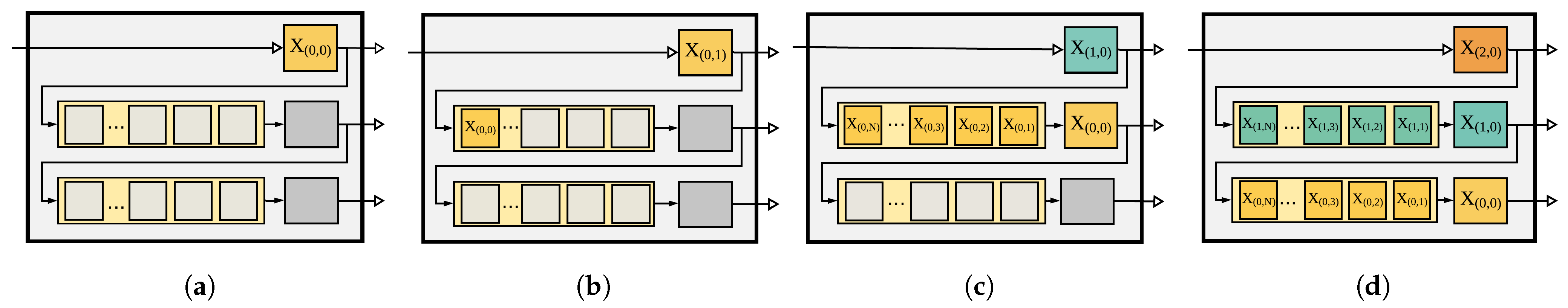
3.2. Boundary Conditions
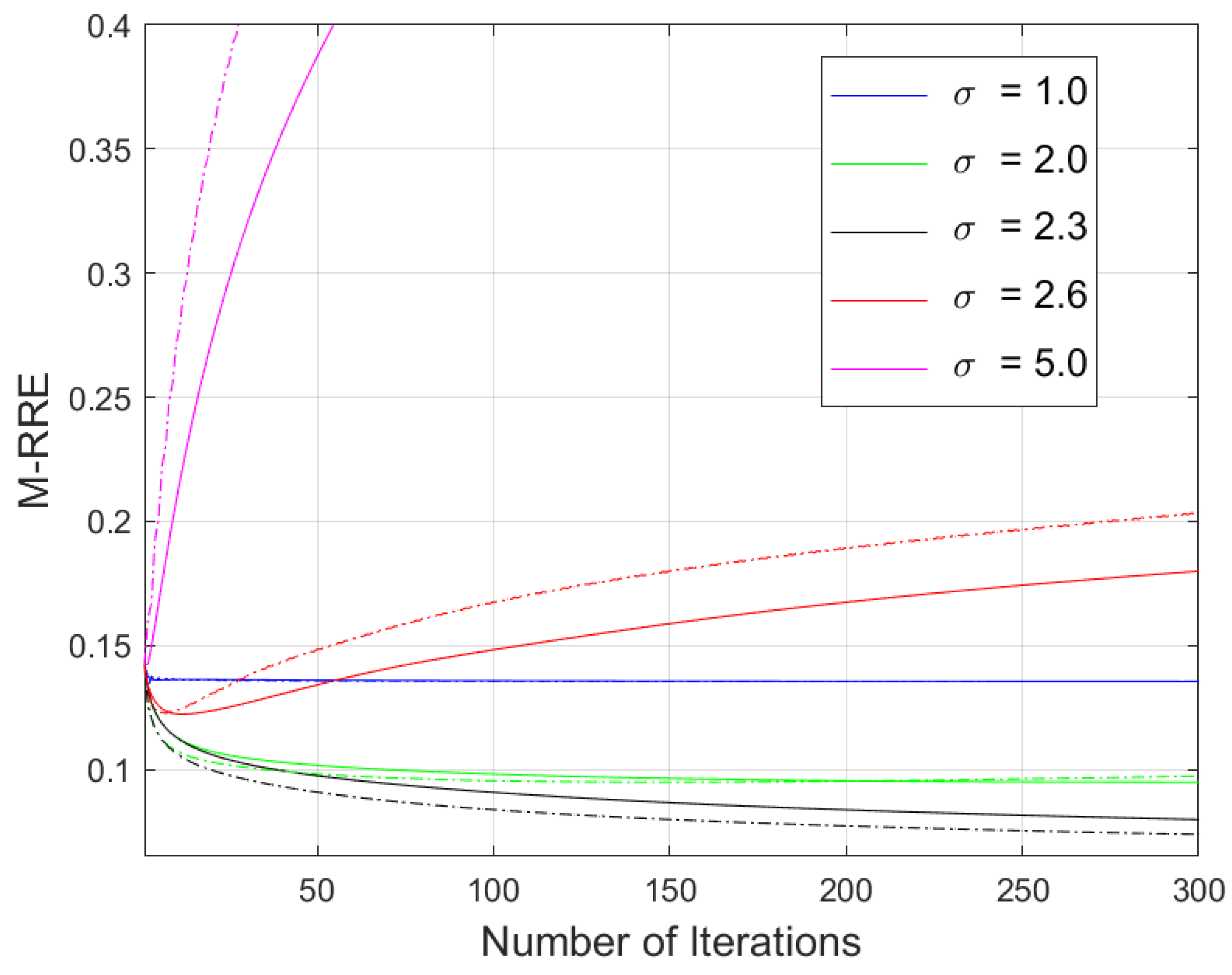
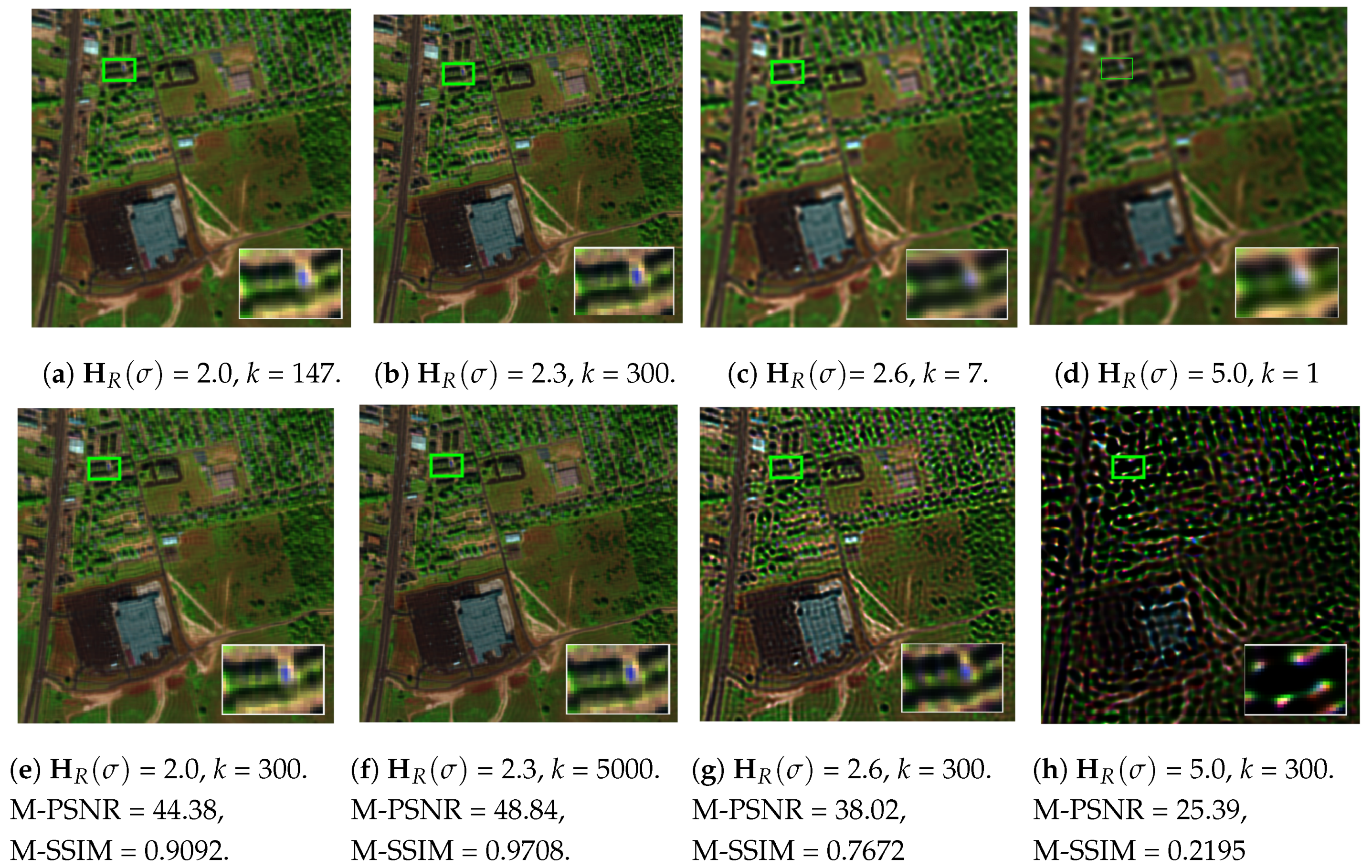
3.3. Effects of Kernel Standard Deviation on Image Reconstruction
4. Proposed Implementation
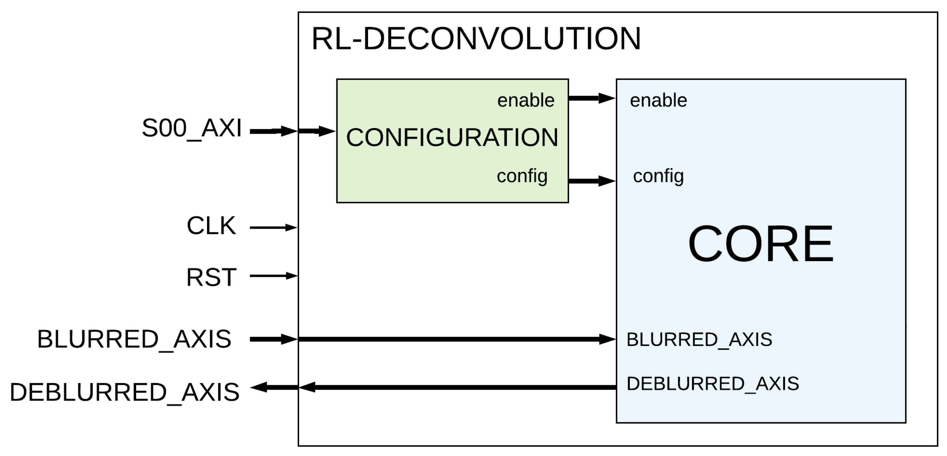
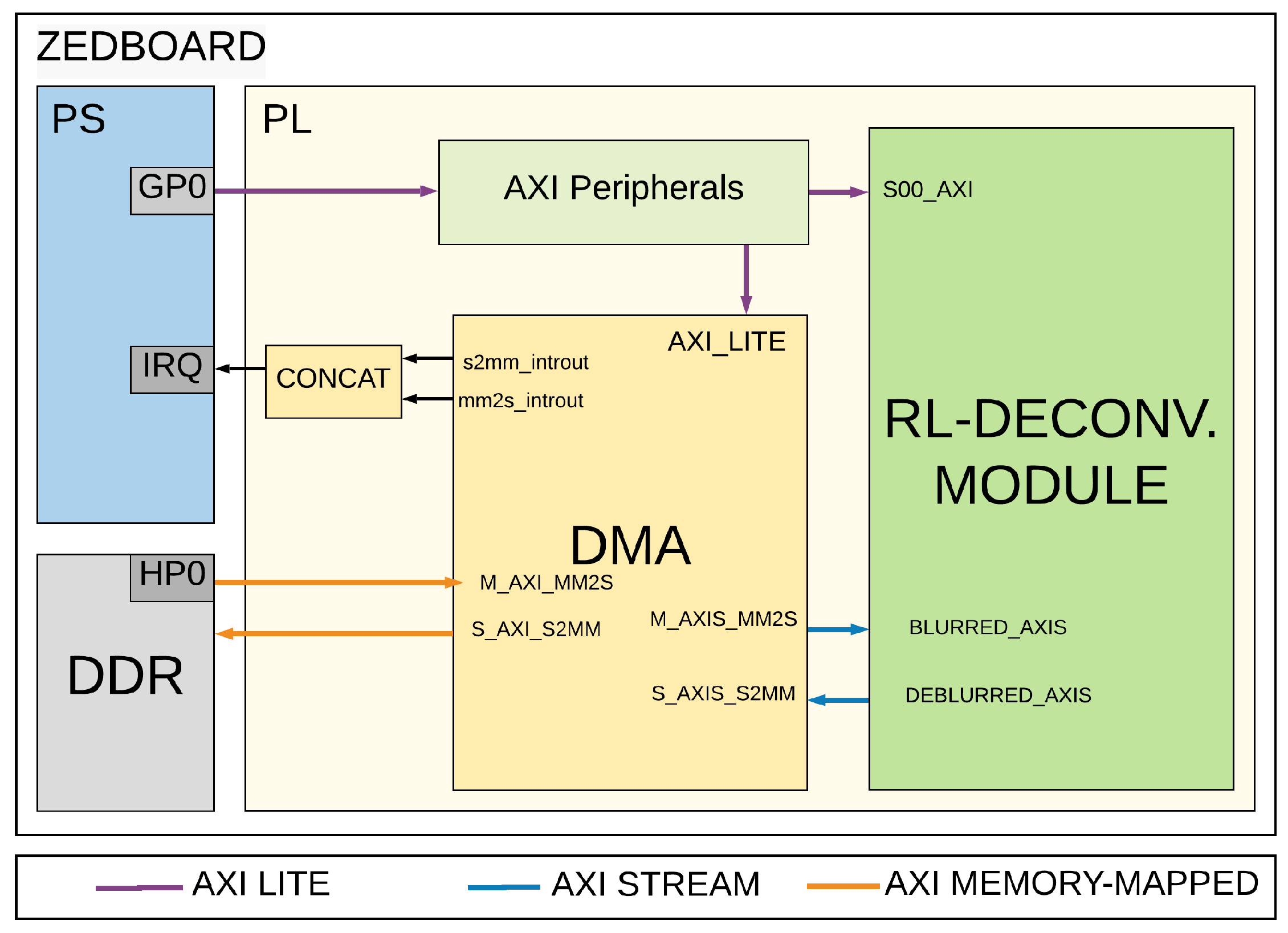
4.1. Overall Architecture
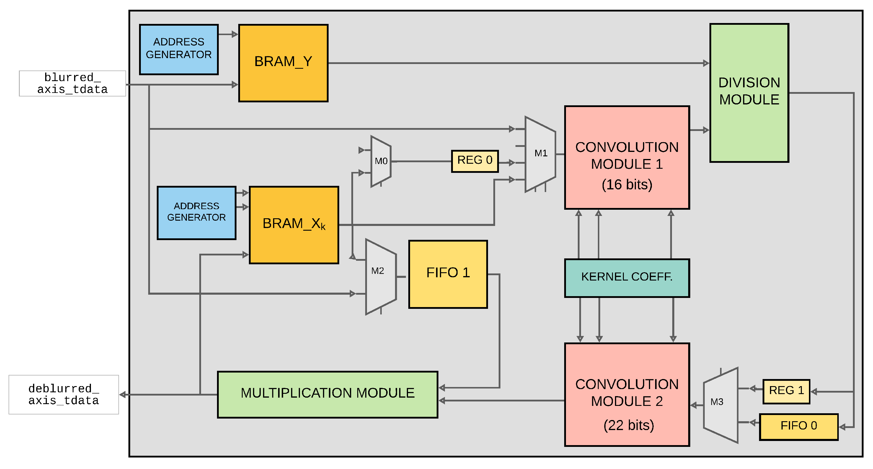
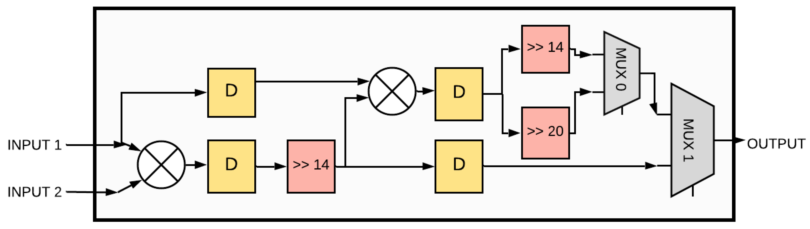
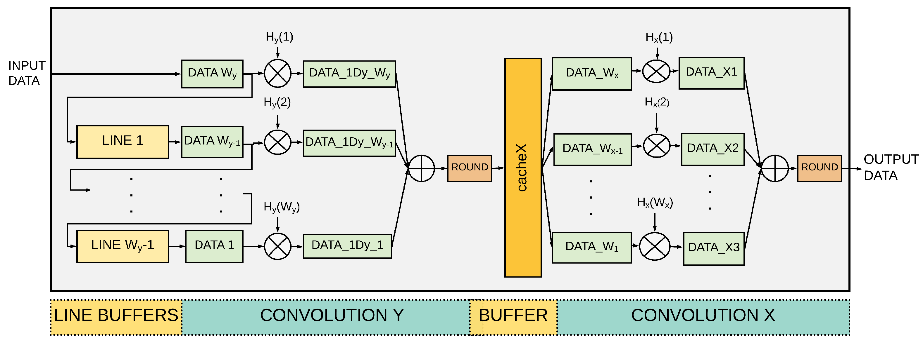
4.2. Convolution Module
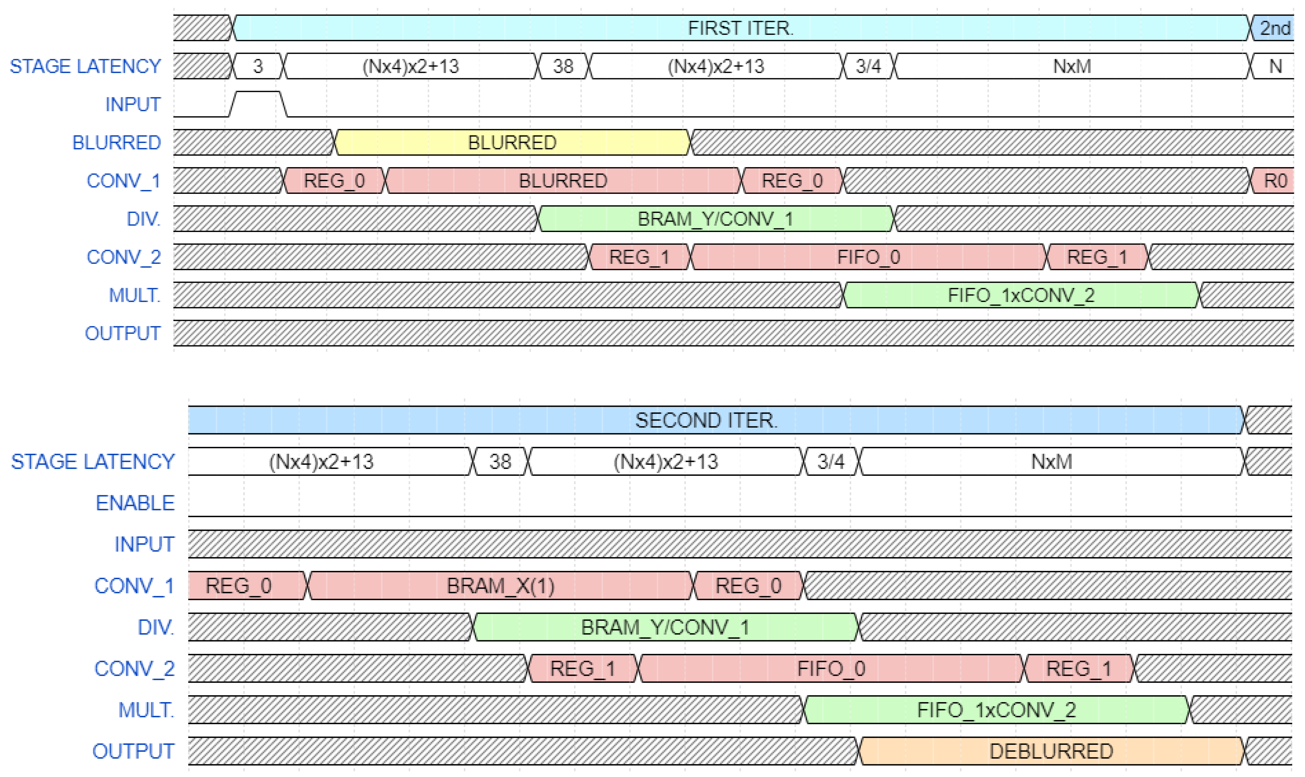
4.3. Data Processing Pipeline
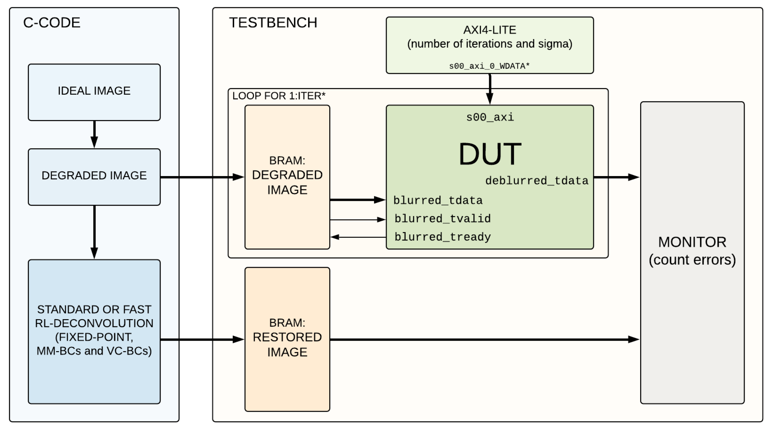
5. Results
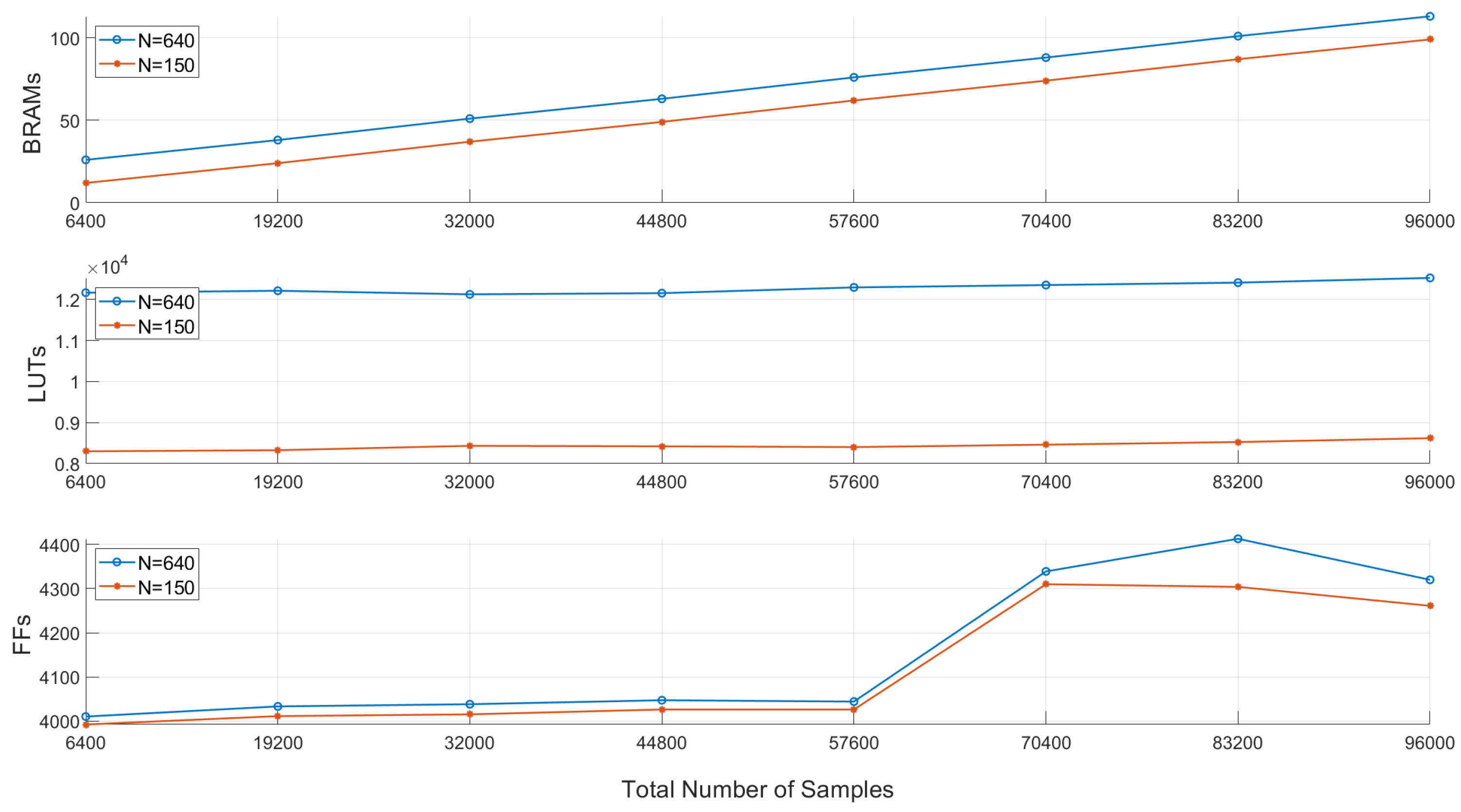
5.1. Resource Utilization
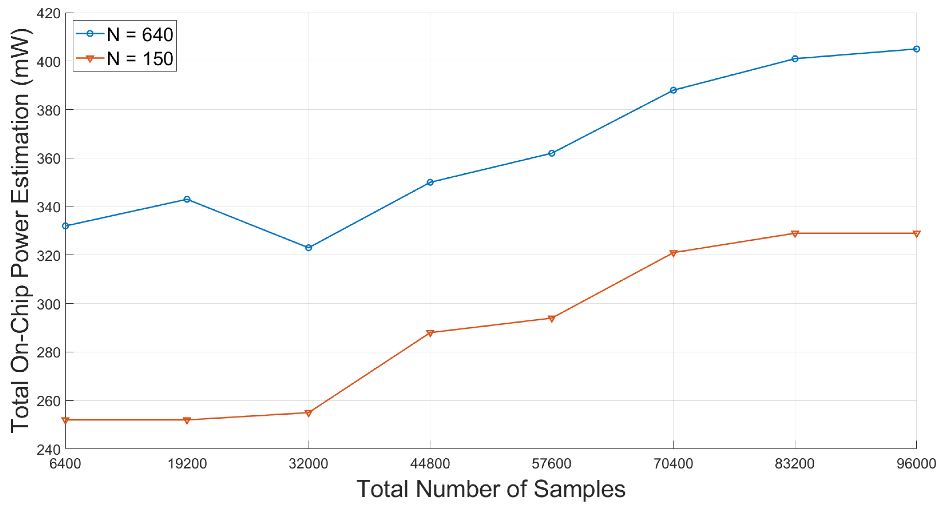
5.2. Power Estimation
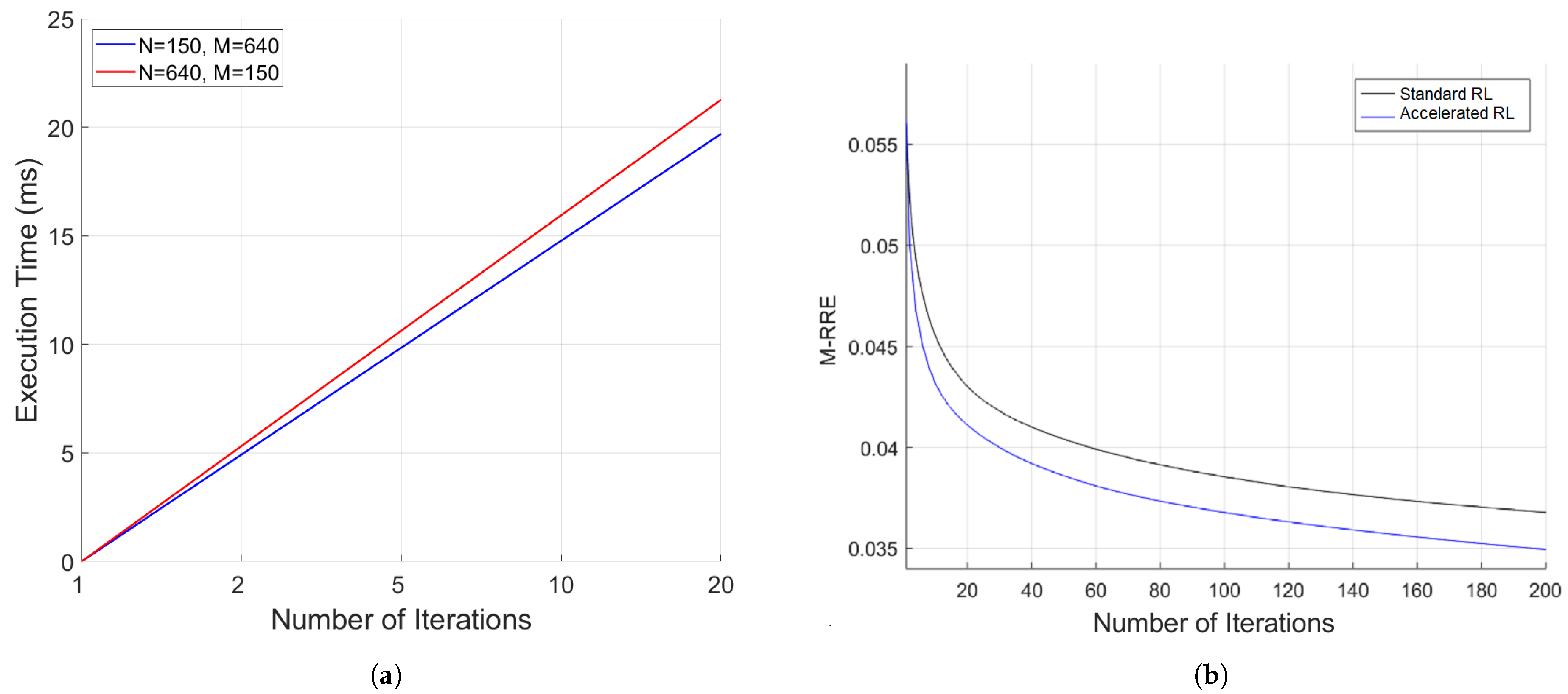
5.3. Execution Time
6. Conclusions
Author Contributions
Funding
Institutional Review Board Statement
Informed Consent Statement
Data Availability Statement
Conflicts of Interest
Sample Availability
References
- Smith, R.B. Introduction to Hyperspectral Imaging; MicroImages: Lincoln, NE, USA, 2006. [Google Scholar]
- Shippert, P. Introduction to Hyperspectral Image Analysis. Online J. Space Commun. 2003, 3, 13. [Google Scholar]
- Richardson, W.H. Bayesian-Based Iterative Method of Image Restoration. J. Opt. Soc. Am. 1972, 62, 55–59. [Google Scholar] [CrossRef]
- Lucy, L.B. An iterative technique for the rectification of observed distributions. Astron. J. 1974, 79, 745–754. [Google Scholar] [CrossRef] [Green Version]
- Gonzalez, R.C.; Woods, R.E. Digital Image Processing, 2nd ed.; Prentice Hall: Upper Saddle River, NJ, USA, 2002. [Google Scholar]
- Dines, K.; Kak, A. Constrained least squares filtering. IEEE Trans. Acoust. Speech Signal Process. 1977, 25, 346–350. [Google Scholar] [CrossRef]
- Hunt, B.; Kubler, O. Karhunen-Loeve multispectral image restoration, part I: Theory. IEEE Trans. Acoust. Speech Signal Process. 1984, 32, 592–600. [Google Scholar] [CrossRef]
- Galatsanos, N.; Chin, R. Digital restoration of multi-channel images. IEEE Int. Conf. Acoust. Speech Signal Process. 1987, 12, 1244–1247. [Google Scholar] [CrossRef]
- Galatsanos, N.P.; Katsaggelos, A.K.; Chin, R.T.; Hillery, A.D. Least squares restoration of multichannel images. IEEE Trans. Signal Process. 1991, 39, 2222–2236. [Google Scholar] [CrossRef]
- Henrot, S.; Soussen, C.; Brie, D. Fast Positive Deconvolution of Hyperspectral Images. IEEE Trans. Image Process. Publ. IEEE Signal Process. Soc. 2012, 22. [Google Scholar] [CrossRef] [PubMed] [Green Version]
- Hunt, B.R. Super-resolution of images: Algorithms, principles, performance. Int. J. Imaging Syst. Technol. 2005, 6, 297–304. [Google Scholar] [CrossRef]
- Jemec, J.; Pernuš, F.; Likar, B.; Bürmen, M. Deconvolution-based restoration of SWIR pushbroom imaging spectrometer images. Opt. Express 2016, 24, 24704–24718. [Google Scholar] [CrossRef]
- Wang, Z.; Weng, K.; Cheng, Z.; Yan, L.; Guan, J. A co-design method for parallel image processing accelerator based on DSP and FPGA. In MIPPR 2011: Parallel Processing of Images and Optimization and Medical Imaging Processing; International Society for Optics and Photonics: Guilin, China, 2011; Volume 8005, p. 800506. [Google Scholar]
- Anacona-Mosquera, O.; Arias-García, J.; Muñoz, D.M.; Llanos, C.H. Efficient hardware implementation of the Richardson-Lucy Algorithm for restoring motion-blurred image on reconfigurable digital system. In Proceedings of the 2016 29th Symposium on Integrated Circuits and Systems Design (SBCCI), Belo Horizonte, Brazil, 29 August–3 September 2016; pp. 1–6. [Google Scholar] [CrossRef]
- Sims, O. Efficient Implementation of Video Processing Algorithms on FPGA. Ph.D. Thesis, University of Glasgow, Glasgow, UK, 2007. [Google Scholar]
- Carrato, S.; Ramponi, G.; Marsi, S.; Jerian, M.; Tenze, L. FPGA implementation of the Lucy-Richardson algorithm for fast space-variant image deconvolution. In Proceedings of the 2015 9th International Symposium on Image and Signal Processing and Analysis (ISPA), Zagreb, Croatia, 7–9 September 2015; pp. 137–142. [Google Scholar] [CrossRef]
- Avagian, K.; Orlandić, M.; Johansen, T.A. An FPGA-oriented HW/SW Codesign of Lucy-Richardson Deconvolution Algorithm for Hyperspectral Images. In Proceedings of the 2019 8th Mediterranean Conference on Embedded Computing (MECO), Budva, Montenegro, 10–14 June 2019; pp. 1–6. [Google Scholar]
- Bertero, M.; Boccacci, P.; Desidera, G.; Vicidomini, G. Image deblurring with Poisson data: From cells to galaxies. Inverse Probl. 2009, 25, 123006. [Google Scholar] [CrossRef]
- Biggs, D.S.; Andrews, M. Acceleration of iterative image restoration algorithms. Appl. Opt. 1997, 36, 1766–1775. [Google Scholar] [CrossRef] [PubMed] [Green Version]
- Meinel, E.S. Origins of linear and nonlinear recursive restoration algorithms. J. Opt. Soc. Am. A 1986, 3, 787–799. [Google Scholar] [CrossRef]
- Lanteri, H.; Roche, M.; Cuevas, O.; Aime, C. A general method to devise maximum-likelihood signal restoration multiplicative algorithms with non-negativity constraints. Signal Process. 2001, 81, 945–974. [Google Scholar] [CrossRef]
- Almeida, M.; Figueiredo, M. Deconvolving Images With Unknown Boundaries Using the Alternating Direction Method of Multipliers. IEEE Trans. Image Process. 2013, 22, 3074–3086. [Google Scholar] [CrossRef] [PubMed] [Green Version]
- Fang, H.; Luo, C.; Zhou, G.; Wang, X. Hyperspectral Image Deconvolution with a Spectral-Spatial Total Variation Regularization. Can. J. Remote Sens. 2017, 43, 384–395. [Google Scholar] [CrossRef]
- Zhu, F.; Wang, Y.; Fan, B.; Meng, G.; Pan, C. Effective Spectral Unmixing via Robust Representation and Learning-based Sparsity. arXiv 2014, arXiv:1409.0685. [Google Scholar]
- X. Inc. Divider Generator (v5.1). 2016. Available online: https://www.xilinx.com/support/documentation/ip_documentation/div_gen/v5_1/pg151-div-gen.pdf (accessed on 27 May 2019).
- X. Inc. FIFO Generator (v13.1). 2017. Available online: https://www.xilinx.com/support/documentation/ip_documentation/fifo_generator/v13_1/pg057-fifo-generator.pdf (accessed on 27 May 2019).
- Orlandić, M.; Svarstad, K. An adaptive high-throughput edge detection filtering system using dynamic partial reconfiguration. J. Real-Time Image Process. 2018, 16, 2409–2424. [Google Scholar] [CrossRef]
- X. Inc. Vivado Design Suite-HLx Editions. 2015. Available online: https://www.xilinx.com/products/design-tools/vivado.html (accessed on 27 May 2019).
- Avnet. ZedBoard, Hardware User’s Guide. 2014. Available online: http://zedboard.org/sites/default/files/documentations/ZedBoard_HW_UG_v2_2.pdf (accessed on 16 December 2018).
- ARM, A. AXI DMA v7.1 LogicCore IP Product Guide. 2018. Available online: https://www.xilinx.com/support/documentation/ip_documentation/axi_dma/v7_1/pg021_axi_dma.pdf (accessed on 10 December 2018).
- Fjeldtvedt, J.; Orlandić, M. CubeDMA–Optimizing three-dimensional DMA transfers for hyperspectral imaging applications. Microprocess. Microsyst. 2019, 65, 23–36. [Google Scholar] [CrossRef]
- X. Inc. 7 Series FPGAs Memory Resources. 2017. Available online: https://www.xilinx.com/support/documentation/user_guides/ug473_7Series_Memory_Resources.pdf (accessed on 20 June 2019).


| BCs | M-PSNR(dB) | M-SSIM | ||
|---|---|---|---|---|
| Relative | Relative | |||
| M-PSNR | Improvement (dB) | M-SSIM | Improvement (%) | |
| Z-BC | 20.75 | −20.37 | 0.7805 | −0.69 |
| VC-BC | 45.00 | 3.85 | 0.8920 | 13.50 |
| MP-BC | 41.37 | 0.23 | 0.8859 | 12.72 |
| iter. | M-PSNR(dB) | M-SSIM | |||
|---|---|---|---|---|---|
| Relative | Relative | ||||
| M-PSNR | Improvement (dB) | M-SSIM | Improvement (%) | ||
| 1.0 | 300 | 41.57 | 0.42 | 0.8025 | 2.12 |
| 2.0 | 294 | 44.61 | 3.46 | 0.8985 | 14.33 |
| 2.3 | 300 | 46.11 | 5.97 | 0.9207 | 17.16 |
| 2.6 | 22 | 42.42 | 1.27 | 0.8287 | 5.45 |
| 5.0 | 1 | 41.14 | 0.0 | 0.7888 | 0.37 |
| iter. | M-PSNR(dB) | M-SSIM | |||
|---|---|---|---|---|---|
| Relative | Relative | ||||
| M-PSNR | Improvement (dB) | M-SSIM | Improvement (%) | ||
| 1.0 | 165 | 41.57 | 0.42 | 0.8027 | 2.14 |
| 2.0 | 147 | 44.61 | 3.64 | 0.8986 | 14.34 |
| 2.3 | 300 | 46.79 | 5.64 | 0.9361 | 19.11 |
| 2.6 | 7 | 42.40 | 1.26 | 0.8293 | 5.52 |
| 5.0 | 1 | 39.85 | −1.29 | 0.7807 | −0.78 |
| Feature | Proposed Architecture |
|---|---|
| Standard RL deconvolution | ✓ |
| Accelerated RL deconvolution | ✓ |
| Initial value, | |
| BCs | MP-BCs |
| Generic image size | ✓ |
| Run-time conf. kernel size | ✓ |
| Run-time conf. number of iterations | ✓ |
| Intermediate image data stored internally | ✓ |
| Iter. | Image Size | PSF | Time | Freq. | Throughput | |
|---|---|---|---|---|---|---|
| (ms) | (MHz) | (Samples/s) | ||||
| [16] | 15 | 640 × 480 | <10 | 40 | - | 115.2 |
| [14] | 10 | 800 × 525 | 9 × 9 | 80 | 61 | 52.5 |
| [13] | 60 | 64 × 64 | 13 × 13 | 78 | 100 | 3.1 |
| SW-Only | 1 | 150 × 480 | 9 × 9 | 60.1 | 100 | 1.6 |
| HW/SW codesign [17] | 1 | 150 × 480 | 9 × 9 | 25.7 | 100 | 3.7 |
| Proposed work, *SoC | 1 | 150 × 640 | 9 × 9 | 0.98 | 100 | 97.96 |
| Proposed work, *SoC | 1 | 640 × 150 | 9 × 9 | 1.06 | 100 | 90.6 |
| Proposed work, max freq. | 1 | 150 × 640 | 9 × 9 | 0.87 | 110 | 110.3 |
Publisher’s Note: MDPI stays neutral with regard to jurisdictional claims in published maps and institutional affiliations. |
© 2021 by the authors. Licensee MDPI, Basel, Switzerland. This article is an open access article distributed under the terms and conditions of the Creative Commons Attribution (CC BY) license (http://creativecommons.org/licenses/by/4.0/).
Share and Cite
Avagian, K.; Orlandić, M. An Efficient FPGA Implementation of Richardson-Lucy Deconvolution Algorithm for Hyperspectral Images. Electronics 2021, 10, 504. https://doi.org/10.3390/electronics10040504
Avagian K, Orlandić M. An Efficient FPGA Implementation of Richardson-Lucy Deconvolution Algorithm for Hyperspectral Images. Electronics. 2021; 10(4):504. https://doi.org/10.3390/electronics10040504
Chicago/Turabian StyleAvagian, Karine, and Milica Orlandić. 2021. "An Efficient FPGA Implementation of Richardson-Lucy Deconvolution Algorithm for Hyperspectral Images" Electronics 10, no. 4: 504. https://doi.org/10.3390/electronics10040504