Article

Deep Learning Methods for Classification of Certain Abnormalities in Echocardiography

1
Department of Information Technology, North-Eastern Hill University, Shillong 793022, Meghalaya, India
2
Techno India NJR Institute of Technology, Udaipur 313003, Rajasthan, India
3
Department of Electrical Engineering Fundamentals, Faculty of Electrical Engineering, Wroclaw University of Science and Technology, 50-370 Wroclaw, Poland
4
Faculty of Law, Administration and Economics, University of Wroclaw, 50-145 Wroclaw, Poland
*
Author to whom correspondence should be addressed.
Electronics 2021, 10(4), 495; https://doi.org/10.3390/electronics10040495
Submission received: 29 January 2021 / Revised: 16 February 2021 / Accepted: 17 February 2021 / Published: 20 February 2021

Abstract

:
This article experiments with deep learning methodologies in echocardiogram (echo), a promising and vigorously researched technique in the preponderance field. This paper involves two different kinds of classification in the echo. Firstly, classification into normal (absence of abnormalities) or abnormal (presence of abnormalities) has been done, using 2D echo images, 3D Doppler images, and videographic images. Secondly, based on different types of regurgitation, namely, Mitral Regurgitation (MR), Aortic Regurgitation (AR), Tricuspid Regurgitation (TR), and a combination of the three types of regurgitation are classified using videographic echo images. Two deep-learning methodologies are used for these purposes, a Recurrent Neural Network (RNN) based methodology (Long Short Term Memory (LSTM)) and an Autoencoder based methodology (Variational AutoEncoder (VAE)). The use of videographic images distinguished this work from the existing work using SVM (Support Vector Machine) and also application of deep-learning methodologies is the first of many in this particular field. It was found that deep-learning methodologies perform better than SVM methodology in normal or abnormal classification. Overall, VAE performs better in 2D and 3D Doppler images (static images) while LSTM performs better in the case of videographic images.

1. Introduction

With the advances in the field of biomedical imaging, digital images play a vital role in the early detection of abnormalities or diseases in the human body for any systems. Many intricate systems exist in the human body, namely the nervous system, cardiac system, endocrine system, etc that are important for survival. Out of these, the cardiac system is considered to be one of the most delicate systems. Cardiology is viewed as a complex subject of practice due to less exposure to the intricacies of relevant technologies. Medical imaging has become a tool for diagnosis purposes and provides information about the anatomic structures with the assistance of computers through imaging modalities like Computed Tomography (CT), Magnetic Resonance Imaging (MRI), Angiogram, Electrocardiograph (ECG) and others [1].
Amongst these, echocardiogram (echo) is considered and perhaps the most frequently used tool in the field of the cardiac system. It is used mainly due to its ability for early diagnosis and management of heart diseases. It is a simple, non-invasive, and inexpensive technique that can precisely show the pressure gradient of heart lesions. Since it uses sound waves instead of radiation, echo is considered to be safe [2]. Echo uses standard two-dimensional (2D), three-dimensional (3D), and Doppler ultrasound to create images of the heart [3]. The echo plays a crucial role in the diagnosis of cardiac diseases. The images used in this work are captured when the patient is in the left lateral decubitus (when the patient is lying on the left side) [4]. The transducer used is transthoracic (without insertion of transducer inside the esophagus) [5,6]. The different parts of the heart are Left Ventricle (LV), Right Ventricle (RV), Left Atrium (LA), and Right Atrium (RA). Some different views/planes involved in echo are Parasternal long-axis view (PLAX), RV inflow view (RVIT), Parasternal short-axis view (PSAX), Apical view, Subcostal view etc. [7]. In PLAX view the transducer is placed towards the right shoulder, whereas the PSAX view is obtained by rotating the transducer by 90° in the clockwise direction from the PLAX view [8]. In the case of RVIT, the sound beam of the transducer is pointed towards the right hip [8]. The apical view is quite similar to the PLAX view. However, the only difference is the image is taken from the apex portion of the heart [8]. The subcostal view can be obtained by placing the transducer towards the left, and the sound beam is projected slightly anteriorly [8]. Echo has become a prominent choice used in the examination of valvular heart diseases (regurgitation). Regurgitation [9] is one of the most common valvular diseases that is characterized by the prominent use of tobacco and alcohol. It can be detected from abnormal flow patterns using color imaging (color flow mapping). The main types of regurgitation are:
  • Mitral Regurgitation (MR): It is the most common valvular involvement in children and rheumatic heart diseases. In color flow, LA size is increased, and the MR jet can be seen [10].
  • Aortic regurgitation (AR): AR is known to be less frequent than MR. But most patients having AR have associated mitral valve disease. It results from distorted aortic leaflets and for which careful analysis of the aortic valve is a must [9]. Color flow and Doppler give an estimate of the severity of AR.
  • Tricuspid Regurgitation (TR): It is often common in people who smoke [11]. It can also be seen in 20% of rheumatic heart disease patients. Using Doppler and color flow, TR can be seen, and depending on the TR jet, the severity of TR can be revealed. The tricuspid valve is similar to that of the mitral valve with more variability [9].
The above mentioned three types of regurgitation are acquired heart disease (cause during one’s lifetime). Not all kinds of regurgitation are known to be acquired, as some can be congenital (presence since birth). In our case, it was observed that all cases of patient data are acquired. Figure 1 shows a Doppler echo having AR, MR, and TR abnormalities respectively. This valvular regurgitation plays a significant role and represents an important cause in mortality and morbidity [9]. The echo plays an essential role in regurgitation assessment and using Doppler echo the presence of the types of regurgitation can be distinguished more distinctively. But this has to be done by a cardiologist by precisely locating and assessing the visualization in the form of video. To detect the presence or absence of any abnormalities, extraction of an image or images from a videographic echo is a necessity. From the visualization of echo, a cardiologist can predict the functions of valves and defective parts, if any. However, It requires trained cardiologists to interpret accurate findings and give reports. Often cardiologists take the help of cauterization [12], which is a surgically invasive and expensive procedure. Usage of automated methods will help in the accurate diagnosis of any heart abnormalities and also reduce the necessity of invasive procedures. There are no automated facilities that can detect the presence of abnormalities or any disease in the heart. Thus, finding a way to treat such abnormalities using automated algorithms is needed. An attempt using machine learning algorithms have been made in the past in which SVM has provided better result using static images. But using videographic images was never explored. For this purpose, work using videography has been introduced to reduce the work of a cardiologist and provide an efficient and effective result as this will help in the early detection and diagnosis of heart diseases.
Usage of deep learning and machine learning techniques help us to a greater extent to handle such fine details. This work aims to classify images into normal and abnormal and the different type of regurgitation. It has been observed that the performance of small architecture is quite similar with the performance of more complex architecture. We wanted to examine the clinical capability of our method in classifying the different types of images. Firstly, an effort has been made to classify the echo images into two classes (i.e., abnormal and normal). Then videographic echo images have been considered for further classifications, based on regurgitation present, using two types of deep learning-based models (i.e., LSTM and VAE-CNN). Firstly, RNN based model using LSTM has been chosen due to its capability in recalling the time and predicting the next image or frame. Another method is using Variational Auto Encoder (VAE) with Convolutional Neural Network (CNN). CNN is used for extracting features and for space reduction. A comparison with well-known SVM methodology is also performed using the static images of the echo.
The main contributions of the paper are as follows:
  • Work based on videographic images has been proposed as an initiative to find out its usefulness in the diagnosis of different types of abnormalities. Videographic images are used for classification into six types of regurgitation and two-class (normal or abnormal) classification.
  • Work on 2D images for classification into normal or abnormal in PLAX view [13] has been done and compared to an existing method, i.e., SVM [14,15].
  • Using color Doppler 3D images, classification into normal or abnormal was done.
  • Using RNN and CNN based VAE deep learning methodologies including an existing technique SVM, used for 2D classification, was done.
  • Classification is performed, using the images captured in the Radiology laboratory and validated with the help of a cardiologist.
Works related to regurgitation classification are described in Section 2. In Section 3, the flowchart of different methodologies used, are explained in brief. Section 4 provides the experimental result and Section 5 consists of the conclusion and future work.

2. Related Works

Work based on the cardiac system has become one of the most popular and aspiring field for many researchers. This is because it is one of the most important system of the human body and is the leading cause for morbidity and mortality in patients with kidney disease in the United States [16]. It is one of the main organs for blood supply and can be called as a manufacturer of blood circulation and thus plays a vital role. During echo visualization, any abnormal inflow or outflow of blood can be a sign of abnormalities or diseases in the heart. For this reason, works related to heart abnormalities have been taken in this paper and are discussed further. Many of the related works are not based on the classification of heart abnormalities but are included as they deal with the classification in the heart-related field.
Work related to cardiac classification can be found in Allan et al. [14], where the classification of Mitral Regurgitation (MR) was carried out using SVM as a classification method with an accuracy of 82% for moderate or severe MR. The apical view was taken for this purpose using a 2D echo with 6993 studies obtained from the Clinical Medical Research Ethics Board of Vancouver Coastal Health [14]. Balaji et al. have done works on the classification of different views of echo wherein [17] parasternal short axis (PSAX), parasternal long axis (PLAX), apical two-chamber (A2C), and apical four-chamber (A4C) was classified using the histogram and statistical features with 87.5% accuracy and in [18], parasternal long axis (PLAX), apical two-chamber (A2C) and apical four-chamber (A4C) was classified using Connected Component Labelling with 94.56% accuracy. Nandagopalan [19], has also worked for view classification where parasternal short axis (PSAX), parasternal long axis (PLAX), apical two-chamber (A2C), and apical four-chamber (A4C) was classified using a proposed method with 96% accuracy. Pinjari [20] used Proximal Isovelocity Surface Area (PISA) method for the classification of mild Mitral Regurgitation (MR), moderate Aortic Regurgitation (AR) and severe Aortic Regurgitation (AR). It was done using color Doppler images where images used were MR and AR. The images were first converted into YCbCr space, and filtering techniques like wiener and Gaussian filters were applied. For the same, Segmentation was done using Fuzzy C Means. Another work can be seen in [21], where heart valve disease for AR is assessed. It is assessed using a gradient, Aortic Stenosis (AS) grading, peak velocity, velocity ratio, Aortic Valve Area (AVA), Indexed AVA, and mean gradient. The type of AS is known based on the ratio obtained. Also, Strunic et al. worked on the classification of murmurs using ANN as a classification technique using heart sound [22]. Many papers have considered Left Ventricle (LV) segmentation as an important aspect in finding abnormalities considering LV as the largest part of the heart where the flow of blood can be witnessed [23,24]. A review work was done on machine learning for heart disease prediction in [25], and work on the classification of heart diseases based on the counts of heart beat could be seen in [26].
Along with these methods, other state-of-art emerging techniques are deep learning like Convolutional Neural Network (CNN), Autoencoders, Recurrent Neural Network (RNN) in different fields of biomedical imaging, and computer vision. Deep learning has several families, including fully connected networks like autoencoders, convolutional neural networks like AlexNet, and LeNet, recurrent neural networks like LSTM, and deep belief networks. Using Deep Learning architecture like CNN has an advantage over other Deep learning methodologies, where features are extracted during the process. These architectures have shown excellent performance in many fields and even gained popularity in the field of segmentation of images.
Works related to normal or abnormal heart images have not been done previously. Such work is necessary to help physicians for identification of the presence or absence of any abnormalities. This work has been taken in this paper with a hope that automated methodologies can reduce human exertion and applicable as a tool in places abstain by an expert or ease the process of diagnosis.
In this paper, work based on classification has been taken as an initial step for the prediction of a specific region of interest. Two types of classification have been carried out, namely, classification into normal and abnormal images and classification into different types of regurgitation.

3. Classification of Heart Abnormalities Using Different Architectures

Classification plays an important role in the prediction of an area or region containing abnormalities for the diagnosis of any disease. It classifies input into different classes. In this work, we have used Long Short Term Memory (LSTM), Variational Autoencoder + Convolutional Neural Network (VAE-CNN) along with SVM are used for classification. The 2D static echo images and 3D static doppler images are classified into two classes namely normal or abnormal. Videographic echo images are also classified into two classes (normal or abnormal) and six-classes of regurgitation using the same methodologies.

3.1. Data Acquisition

The raw data were obtained from a Cardiac Clinic namely Hope Clinic loacated in Shillong, India using echo as a tool under the supervison of specialist in the relevant field. A sample image used in the work is shown in Figure 1. The data obtained are in 2D jpeg images, 3D bitmap images, colored and 2D videographic images in Audio Video Interleave (AVI) format. A total of 120 patient data with abnormality/abnormalities cases and a few normal cases were collected. The different types of abnormalities are MR, AR, TR, and a few having mixture of these. All the data are validated with the help of a cardiologist.

3.2. Image Preprocessing and Data Augmentation

An overall flowchart depicting the working methodologies is shown in Figure 2. Our scheme starts with taking an input image (frame in case of video), which is then cropped and converted into gray scale for 2D classification of images and videos. This conversion is important as grayscale images are more detailed and give a better representation of the image. It is then passed for filtering using the Gaussian filter as in [20]. It was done to remove noise, and unwanted data and Gaussian filter give a comparatively better result. Few images having a mixture of two or more abnormalities were augmented so as to obtain 10 number of patient data for experimental purpose in the case of video classification of 6 classes. Augmentation using cropping has been done.

3.3. Classification Using LSTM, VAE-CNN and SVM Methodologies

The images after preprocessing are then saved into two Comma-Separated Values (CSV) files for the testing and training phase. The training CSV file is used for the training and validation phase consisting of a labelled dataset. The images are then processed using different methodologies (LSTM/VAE-CNN/SVM) for validation purposes. The testing CSV file consists of unlabelled data. After which the test images will be predicted, and the output obtained is class 0 or 1 in the case of two class classification and class 0, 1, 2, 3, 4, 5 in the case of six classes for regurgitation classification.
Steps Involved in Classification of Video
The steps involved in Videographic images are as follows:
  • Extract each frame and operate on each of them. This is known as spatiotemporal deep learning.
  • Each frame is assigned a class in the training and validation phase (labelled frames).
  • Frames are cropped and resized into 224 × 224. The size was chosen randomly based on the previous network, like AlexNet.
  • The training set is then passed into the network (LSTM and VAE-CNN) for classification.
  • Output classes 0, 1, 2, 3, 4, 5 in the case of six-class classification and 0 and 1 in the case of two-class classification were obtained.
  • Testing was done on the remaining unlabelled frames of each video.
  • Steps 3 to 5 are repeated.

3.3.1. Long Short Term Memory (LSTM)

LSTM is an RNN based model. LSTM methods are used in speech and Natural Language Processing (NLP). Since 1997, when Hochreiter introduces LSTM, it has become prevalent in the field of text classification [27]. But this RNN technique has also been found suitable for videos by researchers and can help in predicting the next frame in a video and are applied in many fields of videography [28]. For this reason, this method has been used in our case.
This paper aims to use RNN using LSTM as a variant as it is a better version of RNN [28]. RNN has many variants, including LSTM, GRU, and other modified versions. Here, taking video as input is challenging compared to images as videos are a collection of frames.
LSTM is designed to overcome long term dependencies and to solve the vanishing gradient problem [29]. LSTM improves gradient flow and is most suitable when time is taken as a factor. In a way, LSTM is similar to ResNet (Residual networks) [29].
In this paper, the LSTM model is used without any change in architecture. It has input gate units and output gate units, and the resulting units which are complicated are called memory cell [27]. It also consists of forget gate, memory cell inputs, memory cell output. Gates are used for the memorizing process [30]. A diagram showing the working components of LSTM is shown in Figure 3. The elements of LSTM can be calculated as:
F t = Sigmoid [ W f ( H t 1 , X t ) ]
I t = Sigmoid [ W i ( H t 1 , X t ) ]
G t = Sigmoid [ W g ( H t 1 , X t ) ]
O t = Sigmoid [ W o ( H t 1 , X t ) ]
C t = F t · C t 1 + I t · G t
H t = O t · tanh ( C t )
where F t is the forget gate, I t is the input state, G t is the cell state, W is the weight, H is the output, X is the input, O t is the output of the sigmoid gate, and C t is the cell state. For our purpose, the input is passed to a convolutional layer for feature extraction which is then passed to LSTM architecture, and the output is classified into 0 or 1 (normal or abnormal) class for 2D classification, Doppler classification, and two-class video classification using Sigmoid classifier, and class 0 to 5 for six-class classification of regurgitation for videographic images using softmax classifier.

3.3.2. Variational Autoencoder + Convolutional Neural Network (VAE-CNN)

Combining CNN with other methods help the network excel at spatial relationships [31]. Convolutional layers are a significant building block in deep neural networks. However, the gradient computation of the convolution network remains a challenge in TensorFlow. Many researchers argue that even random convolutions are content [32]. On the other hand, Autoencoder is a powerful generative model that takes CNN idea, which is useful for reconstructing its output through encodings.
The overall diagram of how CNN is combined with VAE is shown in Figure 4. VAE has been taken as a method as it works with a diverse range of data [33]. The overall procedure starts with the input being passed to a convolutional layer with filter size 3 × 3 and stride of 2 × 2 followed by another convolutional layer with the same filter size and no stride. Then it is passed to the Maxpooling layer with size 2 × 2 that helps in reducing the image size which is then passed to a fully connected layer with 4096 nodes. It is then followed by VAE where a first dense layer of 500 is used, followed by another dense layer of 120 and then followed by vector generation of μ and σ , which will produce a sample vector of 30 [33]. μ is mean, and σ is the standard deviation. It is then passed to a classification layer that produces output class using sigmoid and softmax classifiers for two-class and six-class, respectively. It can also be passed to a decoder but was not done, as in our case, our purpose is classification.

3.3.3. Support Vector Machine (SVM) Methodology

SVM is one of the most widely used supervised learning methods for classification in the different fields in medical imaging [14,34,35,36]. SVM is memory efficient and effective in case of high dimensional spaces. It is not only used for classification but for regression as well. For this paper, the SVM methodology was taken from [14]. Although the paper did not mention the type of SVM being used, but for our purpose, SVM with a linear kernel is used as it is popularly used in many fields. The linear kernel can be represented as [37]:
( K ( W , I ) X , X ) = W T I
where W T I is the sum of the inner product. The output class obtained is 0 or 1, 0 for normal (absence of abnormalities) class, and 1 for abnormal (presence of abnormalities) class.
The difference in parameters used in LSTM and VAE-CNN is provided in Table 1. After a brief discussion on the different methods used in this paper, the next section is provided with experimental results and conclusions.

4. Experiment and Result Analysis

The implementation was carried out using jupyter notebook, which is a readily available and open-source web application for python programming language and google colab. The result is divided into two parts, firstly, classification into normal or abnormal, and secondly classification into different types of regurgitations. We have used k fold cross validation as our first approach consisting of varieties of folds (2, 5 and 10). The second approach used here is generalization capability in medical diagnostic where there is no observation in the training phase and no data in the training is in the testing phase [38]. If that is not maintained there might be an astonishing relationship between the obtained status and real identity which results in unrealistic results. Here no data in the training phase is in the testing phase as data here are based on patient data where a patient in the training and validation phase (train-test split) is not used in the testing phase (separate CSV file). Except in two patient cases for six-class classifications, the same data was augmented and kept in the same CSV file. The training data is labelled and the testing data is unlabelled. The optimizer used is Adam and batch size of 50.

4.1. Performance Metrics

Performance metrics are used to evaluate and for checking the quality of performance by the algorithms. Accuracy is considered to be one of the most widely applied performance metrics in classification. The different performance metrics used in the paper are as follows:

4.1.1. Classification Accuracy

It is a measure that calculates the ratio of the correct classification to the total number of samples. For class having the same number of samples, accuracy itself is sufficient as a metric.

4.1.2. Logarithmic Loss

It works by castigating false classification. The lower the loss, the better will be the accuracy. It works well for multi-class classification. Here, Binary crossentropy is used as a loss function.

4.1.3. Confusion Matrix

It is a matrix that describes the complete performance of a model. The following can be calculated based on the confusion matrix.

1. Precision

It is the fraction of True Positives (TP) and False Positives (FP). For two class classification, precision can be calculated using
Precision = TP / TP + FP
For six-class classification precision can be calculated using
P i = TP i TP i + j = 0 i E j i + j = i + 1 5 E j i
where i ranges from 0 to 5.

2. Recall

It represents the fraction of True Positives (TP) and False Negatives (FN). For two-class classification recall ca be calculated as
Recall = TP / TP + FN
For six-class it can be generalized as
R i = TP i TP i + j = 0 i 1 E i j + j = i + 1 5 E i j

3. F1 Score

It is a harmonic mean of precision and recall. For two-class classification it is given by:
F 1 Score = 2 × Precision × Recall Precision + Recall
For six-class classification it can be calculated from recall ( R i ) and precision ( P i ) as:
F i = 2 × P i × R i P i + R i

4.2. Classification into Normal or Abnormal

4.2.1. Dataset

Here, classification into normal or abnormal is carried out using two types of echo images. Obtained data are 2D images in Joint Photographic Experts Group (JPEG) format and 3D color Doppler in BitMap (BMP) format. Data were collected from Hope clinic, Shillong. For the validation phase, 10% of the total data were obtained from the training set used in the training phase. For the testing phase, data are separated in an unused folder (which is later saved in CSV file) where these are tested in the later part after validation. The number of images used for 2D image classification and 3D Doppler image classification is 1070 and 540, respectively. Out of which, 10% is for validation and the rest for training. Excluding these, there are 38 number of 2D images and 10 number of Doppler images for testing purposes. Testing data are separated from training and validation in the experiment for prediction purposes. The total number of 2D images is 1108, and 3D Doppler is 550. For k fold classification the data from all the phases are combined. The k fold cross validation was run multiple times to obtain the same number of data in both the methodologies for plotting the confusion matrix. This is done so that comparison can be made with the same number of data even though the pattern obtained in both cases are different.

4.2.2. Output

Figure 5, Figure 6, Figure 7, Figure 8, Figure 9, Figure 10, Figure 11, Figure 12, Figure 13 and Figure 14 show the confusion matrix for 2D images and 3D color Doppler and Table 2, the result showing accuracy, precision, recall, and F1 Score. From the graph in Figure 15 plotted for all performance metrics and output obtained without k fold, we can conclude that VAE-CNN gives better output in almost all cases. In the case of SVM, in testing for 2D images it is almost equivalent to that of VAE-CNN. In other cases, deep learning methodologies are better compared to SVM in the classification of heart images. It can also be seen that accuracy is better in VAE-CNN, precision in SVM, recall in VAE-CNN, and F1 Score in VAE-CNN for 2D images in the validation phase. In the case of color Doppler, accuracy is better in VAE-CNN, precision in VAE-CNN, recall in SVM, and F1 Score in VAE-CNN in the validation phase. During prediction (testing phase), accuracy in SVM, precision in LSTM, recall in VAE-CNN, and F1 Score in VAE-CNN and SVM is better in the case of 2D images. Overall, VAE-CNN gives a better output compared to the other two methods. Using k fold cross validation, in case of 2D images VAE-CNN performs better in the case of 2 fold and 5 fold and almost equivalent to the others in case of 10 folds. We can also see that for 3D doppler images VAE-CNN performs better compared to LSTM and SVM in all the three folds. Overall, VAE-CNN gives a better output when using k fold which is in the case of generalization classification as well.

4.2.3. Statistical Significance Test

Statistical tests are used for comparison of the classifier. Several statistical tests are available out of which paired T-test has been used for comparison of LSTM and VAE-CNN to that of existing SVM methodology. As k fold cross validation is already considered as a statistical procedure, T-test has not been calculated for the same. It is used for determining the mean of two sets, which is equivalent to zero [39]. It shows the significance of a model by specifying the p-value obtained from the test. Mathematically it can be calculated using:
t = d s 2 / n
where d is the mean difference, s 2 is the sample variance and n is the number of samples.
Based on the statistical test in Table 3, the result obtained by both deep learning methodologies dominates that of SVM. It is done by considering the value of 0.05. From the total 8 cases, 6 cases show statistically significant improvement compared to SVM. In all cases LSTM and VAE-CNN obtained statistical significance improvement over SVM, though in some cases there is not much significance. Only in 1 case of VAE-CNN and 1 case of LSTM, there was no improvement at all. Using the obtained data, the deep learning methodologies are more effective based on the value of the paired T-test. Based on the test of the three methodologies, a difference is observed between the group and therefore is statistically significant.

Summary

Some observations based on this classification are as follows:
  • It can be observed that the traditional method could properly classify the different classes as compared to deep learning methodologies.
  • Using different views and types of image format gives an almost equivalent output, which means that these methods work for any view of echo.

4.3. Classification into Types of Regurgitation

Classification for 6 types of regurgitation has been done using videographic images namely, class 0—mitral regurgitation (MR), class 1—aortic regurgitation (AR), class 2—tricuspid regurgitation(TR), class 3—mitral regurgitation, and tricuspid regurgitation (MR+TR), class 4—aortic regurgitation and mitral regurgitation (AR+MR) and class 5—aortic regurgitation, mitral regurgitation and tricuspid regurgitation (AR+MR+TR). These classes were selected based on data availability of the types of regurgitation. Also, classification into two types, i.e., class 0—normal or class 1—abnormal was done using videographic images.

4.3.1. Dataset

The data obtained were in video format, and for each class, 10 patients’ data were used. The frame ranges from 33 to 150 for each patient. The total number of images used for two-class classification during training is 2430, where 243 are for validation purposes. For the testing phase, the total number of images is 539. The total number of images used for six-class classification during training is 5160, where 516 are for validation purposes. For the testing phase, the total number of images is 736. In the case of k fold cross validation, the data were combined from all the phases. Here too the methodologies were run multiple times to obtain the same number of data in both the methodologies for plotting the confusion matrix.

4.3.2. Output

Two methods, namely, LSTM and VAE-CNN, are used for comparison purposes. It was not compared with other methods as no such work has been done in the same field using video. These two methods were used to check the applicability of deep learning methodologies in these fields. From the output obtained in Table 4, Table 5 and Table 6 and graphs in Figure 16 and Figure 17, it could be seen that classification into normal or abnormal gives very accurate results for both the methodologies in the training and validation phase. When it comes to prediction using VAE-CNN, a better result is obtained. Both cases under performed as accuracy during prediction could not be more than 80% in the case of two-class classification. Nonetheless, it can be observed that deep learning methodologies could classify correctly with the highest of 100% accuracy during validation and 95% accuracy during testing/prediction in six-class classification using LSTM. It can also be observed from the output in Figure 18, Table 6, Table 7 and Table 8, and graphs plotted in Figure 19 and Figure 17 that classification into 6 types of regurgitation give better accuracy and overall performance than that of normal or abnormal classification. This is due to the higher similarities pattern between classes. Few examples showing classification into six-class regurgitation can be seen in Figure 20.
Using k fold cross validation it can be observed that LSTM performed better compared to VAE-CNN in both cases (normal or abnormal and types of regurgitation classification). In the case of two-class classification LSTM gives a 100% accuracy score in all three folds while VAE-CNN gives 99% and 98% unlike in the generalization approach. In the case of six-class classification VAE-CNN gives a different result than the generalization approach, where the accuracy is improved and with the best accuracy of 86%. VAE-CNN did not under perform, but could not overtake LSTM in either of the cases.

Summary

It could be observed that accuracy, precision, recall, and F1 score is better in the validation phase for two-class classification than that of six-class classification. Another output could be observed in the testing phase (generalization aprroach) where LSTM is found to be better than VAE-CNN using color Doppler for six-class classification. In the testing phase (generalization approach), the output of VAE-CNN is better than of LSTM for the two-class classification. Low accuracy can occur due to fewer data used. Overall, deep learning can be applied and used instead of the SVM method.
With the number of images increases, VAE performance too increases. For all other cases, the pattern of output is similar or the same except in six-class classification where LSTM performs better in case of testing using generalization approach (train test split and prediction). This is due to inadequate patient data available where few repetitive data had to be used for two different classes. This causes misclassification where a patient having both AR and MR is treated to have only MR or AR. This shows that VAE cannot classify properly for classes having two abnormalities in the same frame. LSTM performs better using video images compared to VAE-CNN. LSTM performs better since it is an RNN based method, it has time as a factor that can predict what is the next class based on the present and previous inputs. LSTM sometimes fails to classify images of the different class taking the previously obtained classes as the next class. Varying encoding on every single pass makes VAE-CNN difficult to classify frames of the same class which is its disadvantage. However, VAE-CNN has both the property of CNN and VAE which provides a continuous latent space and made interpolation simpler and sampling easier. In conclusion, we can say VAE-CNN gives better output using static images and LSTM using videographic images from k fold cross validation and generalization approach.

5. Conclusions and Future Work

Heart abnormalities classification has been little explored in the field of cardiology. It is an important aspect for detecting any future diseases. Any step that makes diagnosis more accessible and a tool in the future for human intervention can never be considered vague. Several works have been done in the past, but using deep learning methodologies or machine learning models has not been explored much in this field. This paper presented two such methodologies in quest of a better algorithm that can better classify the types of regurgitation and class consisting of abnormalities and without any abnormalities. From the obtained output, it can be concluded that using deep learning methodologies regurgitation can be better classified as compared to a well-known SVM method. Using LSTM and VAE prove to be an efficient and effective way in abnormalities detection where the accuracy in most cases is high. Using such algorithms provide a solution to a cardiologist and ease the process of diagnosis. This will reduce human effort and can be used in early detection and for better diagnosis. In this paper, we have used clinical data, not process data, which could be the reason for lesser than expected accuracy in some cases. Work can be done to achieve a greater number of properly processed data in the future using the videographic echo with keyframe extraction and segmentation. This paper is an initiative for the application of deep learning in such kind of works, which can be further expanded. More experiments are needed for a better diagnosis that can ease and even replace human exertion to some extent.

Author Contributions

Conceptualization, I.W. and A.K.M.; methodology, I.W.; software, I.W.; validation, A.K.M. and G.S.; formal analysis, I.W.; investigation, I.W.; writing—original draft preparation, I.W.; writing—review and editing, A.K.M., M.J. and P.C.; supervision, A.K.M., G.S., P.C., M.J., Z.L. and E.J.; Funding acquisition, Z.L. and E.J.; project administration, A.K.M. and G.S. All authors have read and agreed to the published version of the manuscript.
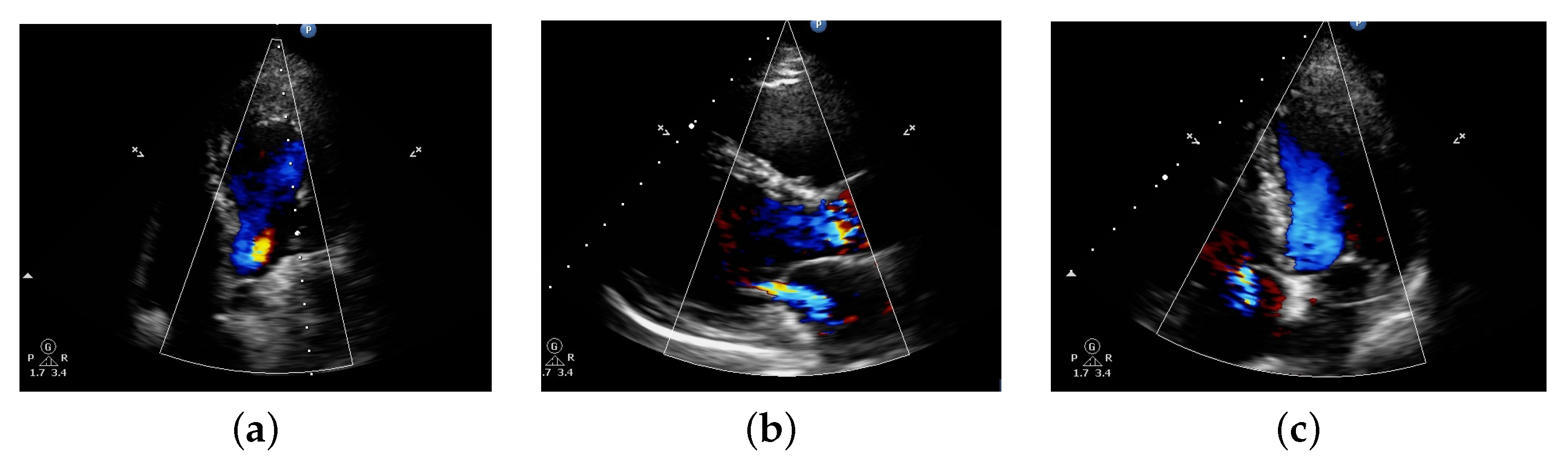
Funding

Publication of this article was financially supported by the Chair of Electrical Engineering, Wroclaw University of Science and Technology.

Data Availability Statement

Limited data available on request due to the large size of the data.

Acknowledgments

A special appreciation and thanks go to D. S. Sethi, Director of Hope clinic, Shillong, India for providing the data and for evaluation and identification of the different types of abnormalities.

Conflicts of Interest

The authors declare no conflict of interest.

References

  1. Mayoclinic: Heart Disease. Available online: https://www.mayoclinic.org/diseases-conditions/heart-disease/diagnosis-treatment/drc-20353124 (accessed on 7 April 2019).
  2. Phoenixheartcenter: Echocardiograms: Transthoracic (TTE) & Transesophageal (TEE). Available online: http://www.phoenixheartcenter.com/echocardiograms-tte-tee/ (accessed on 7 April 2019).
  3. Wikipedia: Echocardiography. Available online: https://en.wikipedia.org/wiki/Echocardiography (accessed on 5 April 2019).
  4. Echocardiography for Emergency Physicians. Available online: https://www.acep.org/sonoguide/cardiac.html (accessed on 5 April 2019).
  5. Transthoracic and Transesophogeal Echocardiography (TEE) and Stress-Echo. Available online: https://www.tcavi.com/services/transthoracic-and-transesophogeal-echocardiography-and-stress-echo/ (accessed on 5 March 2020).
  6. Rowin, E.J.; Maron, B.J.; Haas, T.S.; Garberich, R.F.; Wang, W.; Link, M.S.; Maron, M.S. Hypertrophic cardiomyopathy with left ventricular apical aneurysm: Implications for risk stratification and management. Am. Coll. Cardiol. 2017, 69, 761–773. [Google Scholar] [CrossRef] [PubMed]
  7. Normal Echocardiographic View & Anatomy. Available online: http:==www:ksecho:org=workshop=2017fallw=file=program=26%20Normal:pdf (accessed on 5 April 2019).
  8. Sonography Resources. Available online: https://sites.austincc.edu/sonography-resources/ (accessed on 13 February 2021).
  9. Lancellotti, P.; Tribouilloy, C.; Hagendorff, A.; Popescu, B.A.; Edvardsen, T.; Pierard, L.A.; Badano, L.; Zamorano, J.L. Recommendations for the echocardiographic assessment of native valvular regurgitation: An executive summary from the European association of cardiovascular imaging. Eur. Heart J. Cardiovasc. Imaging 2013, 14, 611–644. [Google Scholar] [CrossRef] [PubMed] [Green Version]
  10. Perloff, J.K.; Marelli, A. The Clinical Recognition of Congenital Heart Disease, 3rd ed.; Jaypee Brothers: New Delhi, India, 2015; pp. 166–678. [Google Scholar]
  11. Gera, R.M. Step by Step Pediatric Echocardiography, 3rd ed.; Jaypee Brothers: New Delhi, India, 2015; pp. 10–80. [Google Scholar]
  12. Healthy Living. Cardiac Catheterization. Available online: https://www.heart.org/en/health-topics/heart-attack/diagnosing-a-heart-attack/cardiac-catheterization (accessed on 9 March 2020).
  13. Family Practice Notebook: Parasternal Long-Axis Echocardiogram View. Available online: https://fpnotebook.com/cv/Rad/PrstrnlLngAxsEchcrdgrmVw.htm (accessed on 5 March 2020).
  14. Allan, G.; Nouranian, S.; Tsang, T.; Seitel, A.; Mirian, M.; Jue, J.; Hawley, D.; Fleming, S.; Gin, K.; Swift, J.; et al. Simultaneous analysis of 2d echo views for left atrial segmentation and disease detection. IEEE Trans. Med. Imaging 2017, 36, 40–50. [Google Scholar] [CrossRef] [PubMed]
  15. Afshin, M.; Ayed, I.B.; Punithakumar, K.; Law, M.; Islam, A.; Goela, A.; Peters, T.; Li, S. Regional assessment of cardiac left ventricular myocardial function via MRI statistical features. IEEE Trans. Med. Imaging 2013, 33, 481–494. [Google Scholar] [CrossRef] [PubMed]
  16. Diabetes/Kidney/Heart Disease. Cardiology Clinics. Available online: https://www.cardiology.theclinics.com/article/S0733-8651(19)30037-2/pdf (accessed on 5 April 2019).
  17. Balaji, G.N.; Subashini, T.S.; Chidambaram, N. Automatic classification of cardiac views in echocardiogram using histogram and statistical features. Procedia Comput. Sci. 2015, 46, 1569–1576. [Google Scholar] [CrossRef] [Green Version]
  18. Balaji, G.N.; Subashini, T.S.; Suresh, A. An efficient view classification of echocardiogram using morphological operations. J. Theor. Appl. Inf. Technol. 2014, 67, 732–735. [Google Scholar]
  19. Nandagopalan, S. Efficient and Automated Echocardiographic Image Analysis through Data Mining Techniques. Ph.D. Thesis, Amrita Vishwa Vidyapeetham University, Amritanagar, India, 2012. [Google Scholar]
  20. Pinjari, A.K. Image Processing Techniques in Regurgitation Analysis. Available online: http://shodhganga.inflibnet.ac.in:8080/jspui/handle/10603/10102 (accessed on 25 July 2013).
  21. Baumgartner, H.; Hung, J.; Bermejo, J.; Chambers, J.B.; Edvardsen, T.; Goldstein, S.; Lancellotti, P.; LeFevre, M.; Miller, F., Jr.; Otto, C.M. Recommendations on the echocardiographic assessment of aortic valve stenosis: A focused update from the european association of cardiovascular imaging and the american society of echocardiography. Eur. Heart J. Cardiovasc. Imaging 2016, 2318, 254–275. [Google Scholar]
  22. Strunic, S.L.; Rios-Gutiérrez, F.; Alba-Flores, R.; Nordehn, G.; Bums, S. Detection and classification of cardiac murmurs using segmentation techniques and artificial neural networks. In Proceedings of the IEEE Symposium on Computational Intelligence and Data Mining, Honolulu, HI, USA, 1–5 April 2007; pp. 397–404. [Google Scholar]
  23. Samaneh, M.; Wirza, R.; Sulaiman, P.S.; Dimon, M.Z.; Khalid, F.; Tayebi, R.M. Segmentation methods of echocardiography images for left ventricle boundary detection. J. Comput. Sci. 2015, 11, 957–970. [Google Scholar]
  24. Naing, O.Y.; Khaing, A.S. Left ventricle segmentation from heart echo images using image processing techniques. Int. J. Sci. Eng. Technol. Res. 2014, 3, 1606–1612. [Google Scholar]
  25. Aljanabi, M.; Qutqut, H.M.; Hijjawi, W. Machine learning classification techniques for heart disease prediction: A review. Int. J. Eng. Technol. 2018, 7, 5373–5379. [Google Scholar]
  26. Alarsan, F.I.; Younes, M. Analysis and classification of heart diseases using heartbeat features and machine learning algorithms. J. Big Data 2019, 6, 1–15. [Google Scholar] [CrossRef] [Green Version]
  27. Hochreiter, S.; Schmidhuber, J. Long short-term memory. Neural Comput. 1997, 9, 1735–1738. [Google Scholar] [CrossRef] [PubMed]
  28. Long Short-Term Memory. Available online: http://axon.cs.byu.edu/martinez/classes/778/Papers/lstm.pdf (accessed on 10 April 2019).
  29. Recurrent Neural Networks. Available online: http://cs231n.stanford.edu/slides/2017/cs231n_2017_lecture10.pdf (accessed on 10 April 2019).
  30. Long Short-Term Memory. Available online: https://towardsdatascience.com/understanding-lstm-and-its-quick-implementation-in-keras-for-sentiment-analysis-af410fd85b47 (accessed on 10 April 2019).
  31. Sequence Classification with LSTM Recurrent Neural Networks in Python with Keras. Available online: https://machinelearningmastery.com/sequence-classification-lstm-recurrent-neural-networks-python-keras/ (accessed on 10 April 2019).
  32. Martin, A.; Chu, A.; Goodfellow, I.; McMahan, H.B.; Mironov, I.; Talwar, K.; Zhang, L. Deep learning with differential privacy. In Proceedings of the 2016 ACM SIGSAC Conference on Computer and Communications Security, Vienna, Austria, 24–28 October 2016; pp. 308–318. [Google Scholar]
  33. Intuitively Understanding Variational Autoencoders. Available online: https://towardsdatascience.com/intuitively-understanding-variational-autoencoders-1bfe67eb5daf (accessed on 9 April 2019).
  34. Taie, S.; Ghonaim, W. CSO-based algorithm with support vector machine for brain tumor’s disease diagnosis. In Proceedings of the IEEE International Conference on Pervasive Computing and Communications Workshops (PerCom Workshops), Kona, HI, USA, 13–17 March 2017; pp. 183–188. [Google Scholar]
  35. Balasubramanian, C.; Sudha, B. Comparative study of de-noising, segmentation, feature extraction, classification techniques for medical images. Int. J. Innov. Res. Sci. Eng. Technol. 2014, 3, 1194–1199. [Google Scholar]
  36. Nelly, G.; Montseny, E.; Sobrevilla, P. State of the art survey on MRI brain tumor segmentation. Magn. Resonance Imaging 2013, 1426–1438. [Google Scholar]
  37. Intelligent Systems: Reasoning and Recognition. Available online: https://ensimag.grenoble-inp.fr/fr/formation/intelligent-systems-reasoning-and-recognition-4mmsirr6 (accessed on 11 February 2019).
  38. Badža, M.M.; Barjaktarović, M.C. Classification of Brain Tumors from MRI Images Using a Convolutional Neural Network. Appl. Sci. 2020, 10, 1999. [Google Scholar] [CrossRef] [Green Version]
  39. T-test using Python and Numpy. Available online: https://towardsdatascience.com/inferential-statistics-series-T-test-using-numpy-2718f8f9bf2f (accessed on 10 February 2019).
Figure 1. Diagram showing Doppler echo from dataset collected of patient having (a) Aortic Regurgitation (AR), (b) Mitral Regurgitation (MR), and (c) Tricuspid Regurgitation (TR) abnormalities respectively.
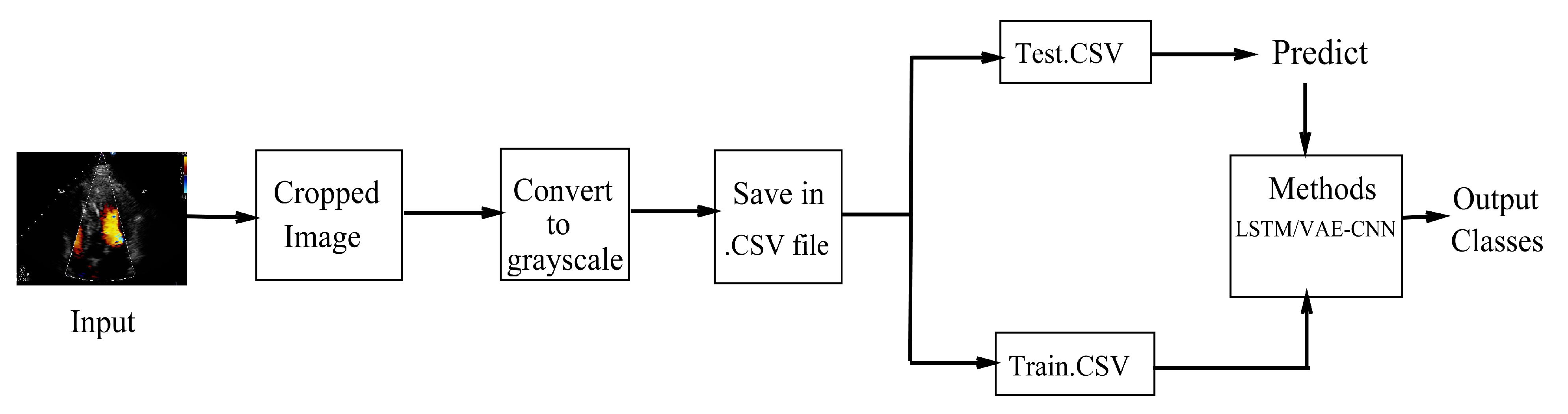
Electronics 10 00495 g001
Figure 2. An overall flow chart showing the working methodologies used in our scheme.
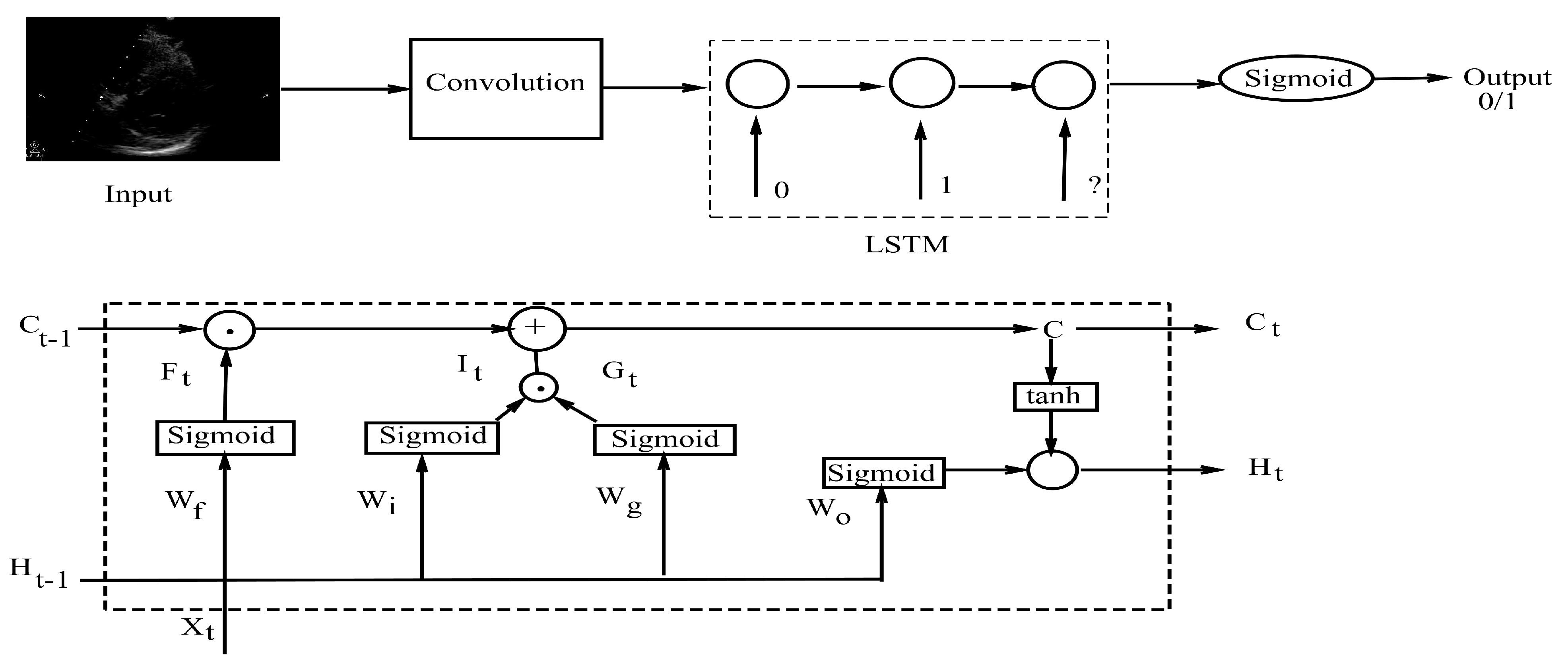
Electronics 10 00495 g002
Figure 3. Long Short Term Memory (LSTM) diagram with an overall flowchart of how the model works where an input image is passed to a convolution layer, then it is forwarded to the architecture whereby images are classified based on the previous and present classification.
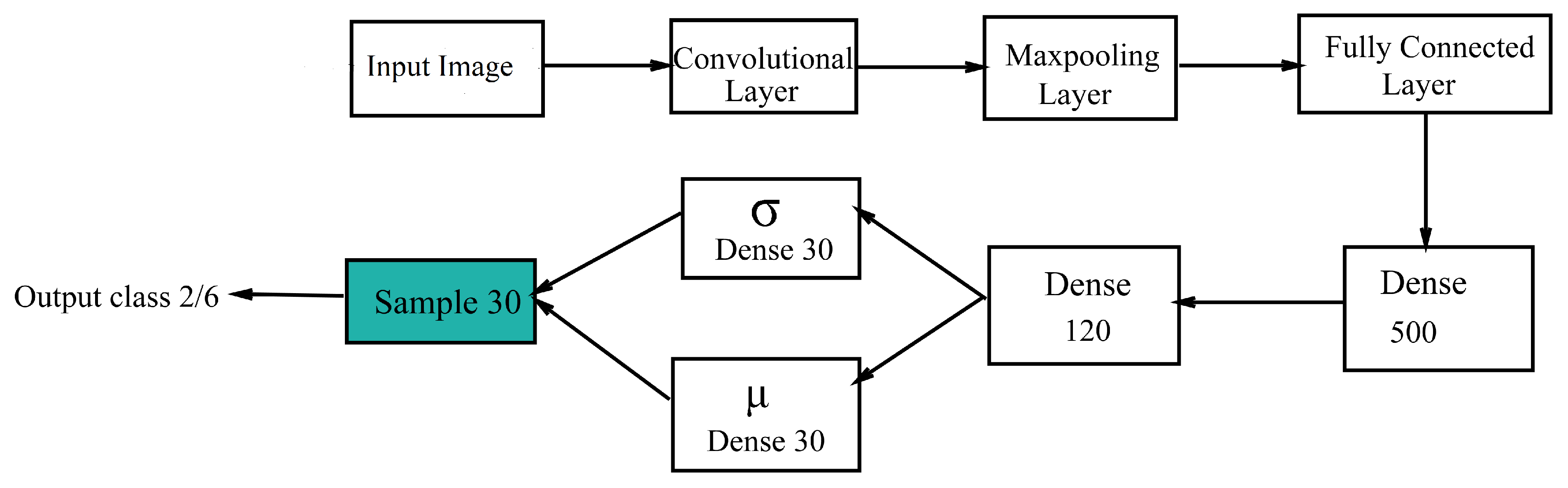
Electronics 10 00495 g003
Figure 4. Variational Autoencoder + Convolutional Neural Network (VAE-CNN) flowchart.
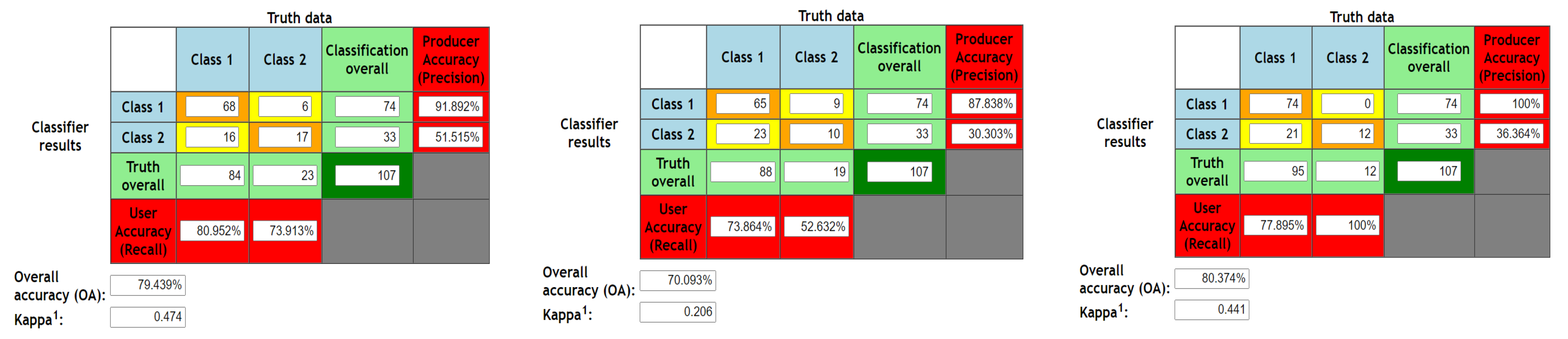
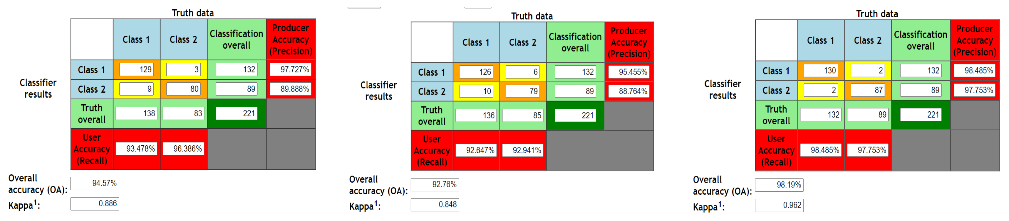
Electronics 10 00495 g004
Figure 5. Confusion matrix for validation phase of 2D images for SVM, LSTM and VAE3CNN respectively.
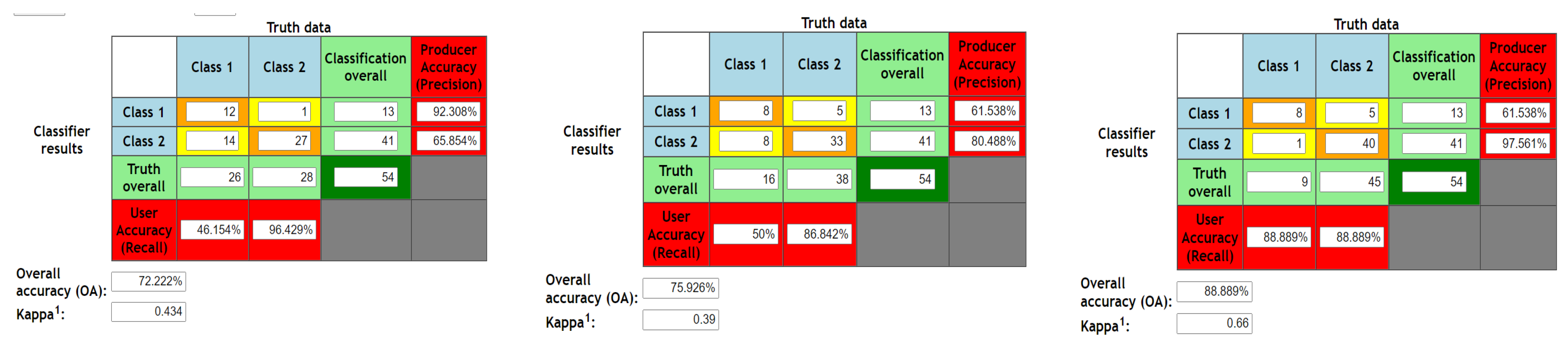
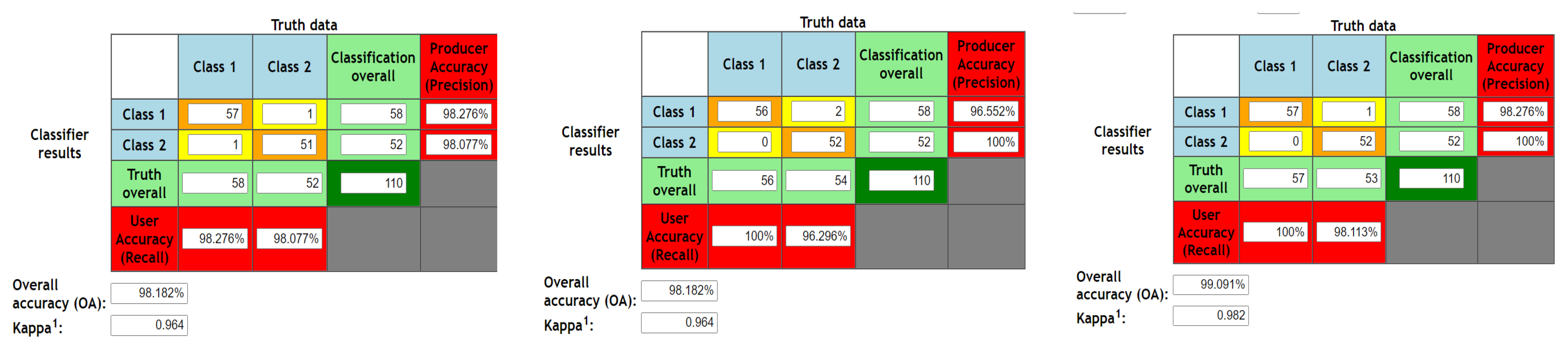
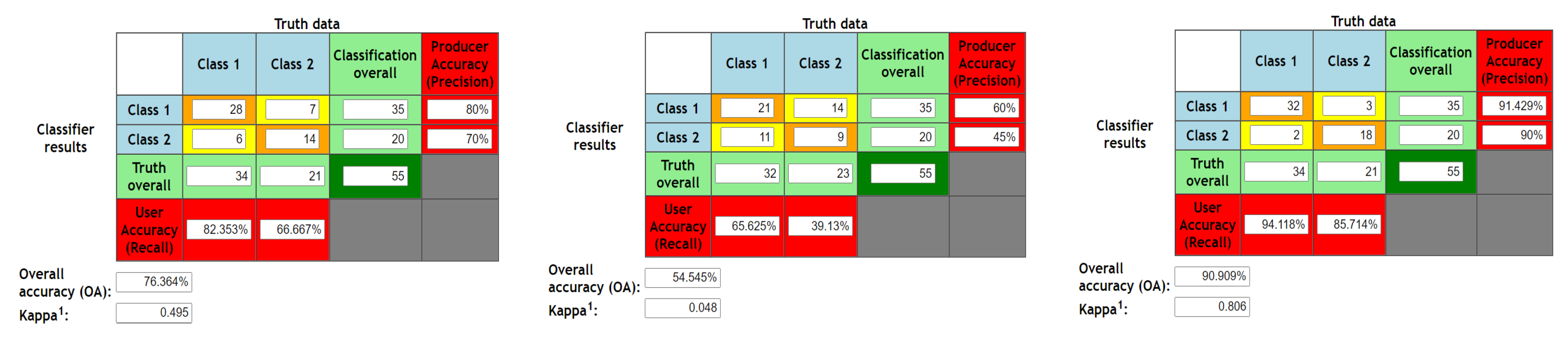
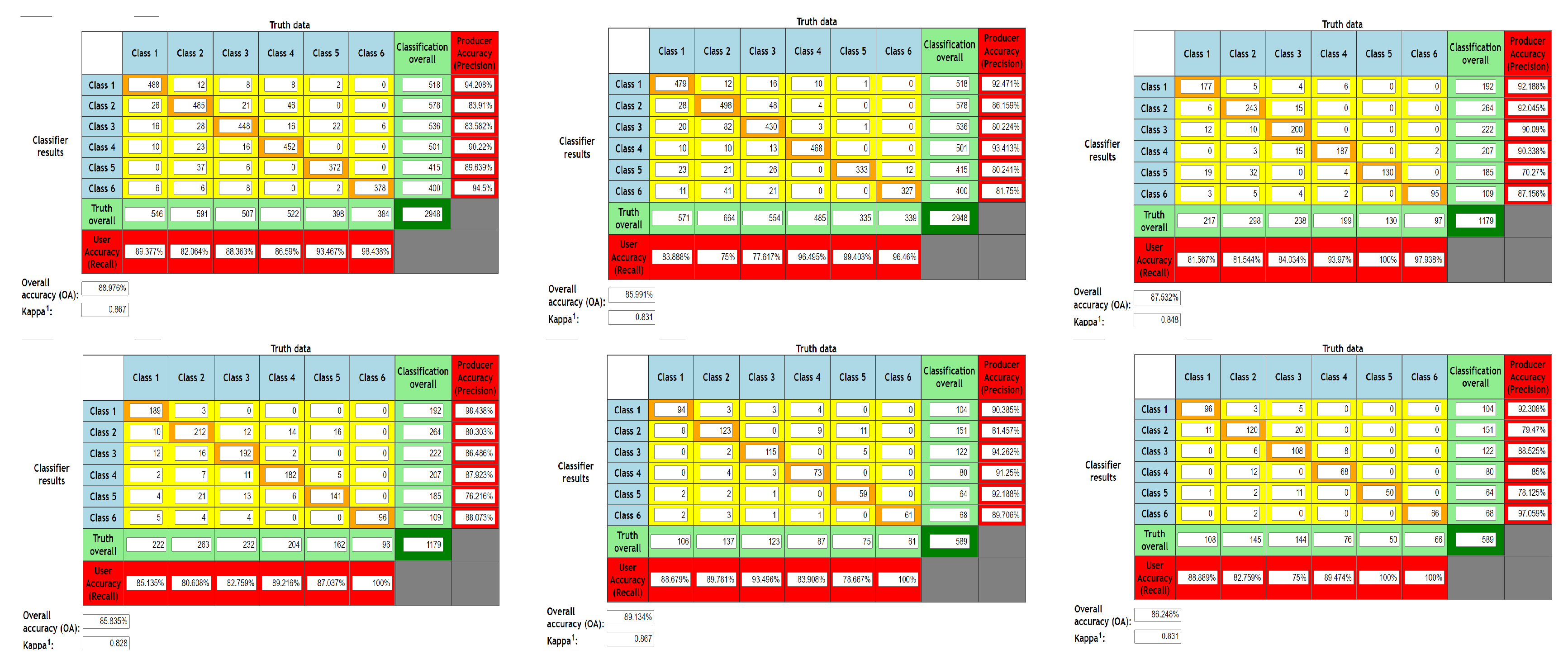
Electronics 10 00495 g005
Figure 6. Confusion matrix for testing phase of 2D images for SVM, LSTM and VAE-CNN respectively.
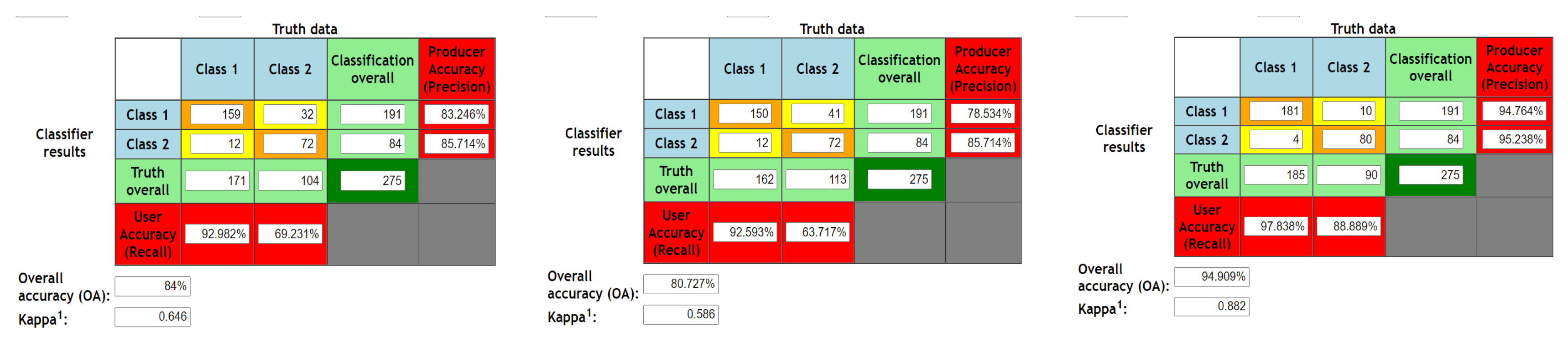
Electronics 10 00495 g006
Figure 7. Confusion matrix for Validation phase of 3D Doppler images for SVM, LSTM and VAE-CNN respectively.
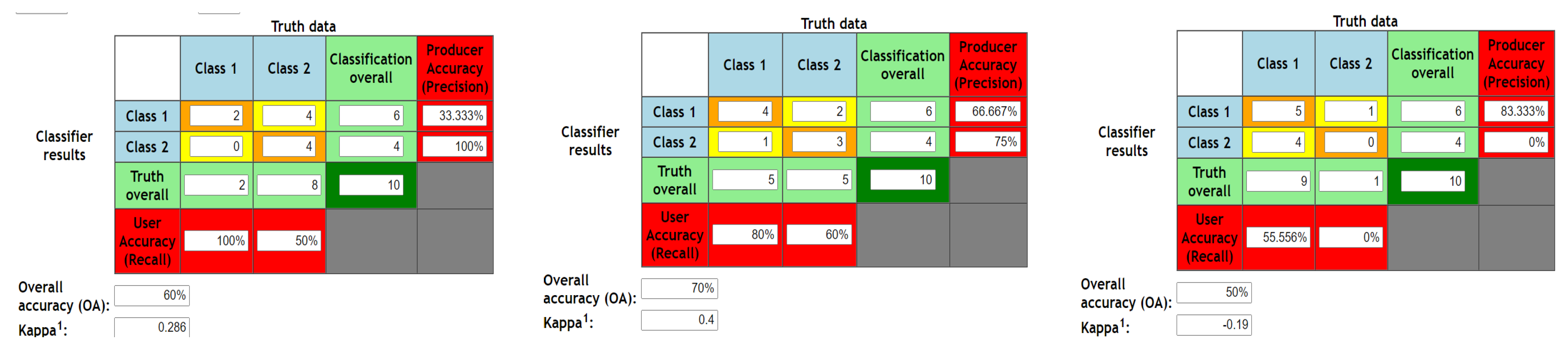
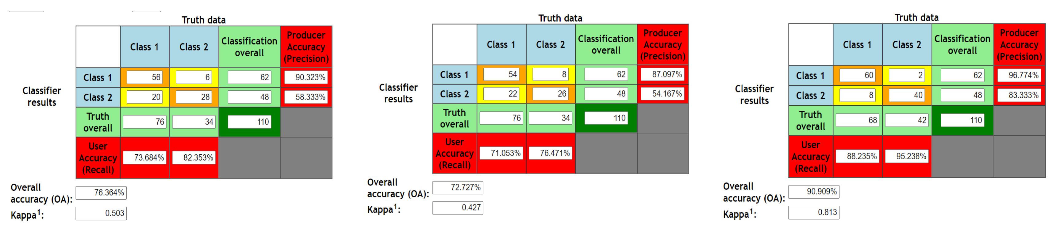
Electronics 10 00495 g007
Figure 8. Confusion matrix for testing phase of 3D Doppler images for SVM, LSTM and VAE-CNN respectively.
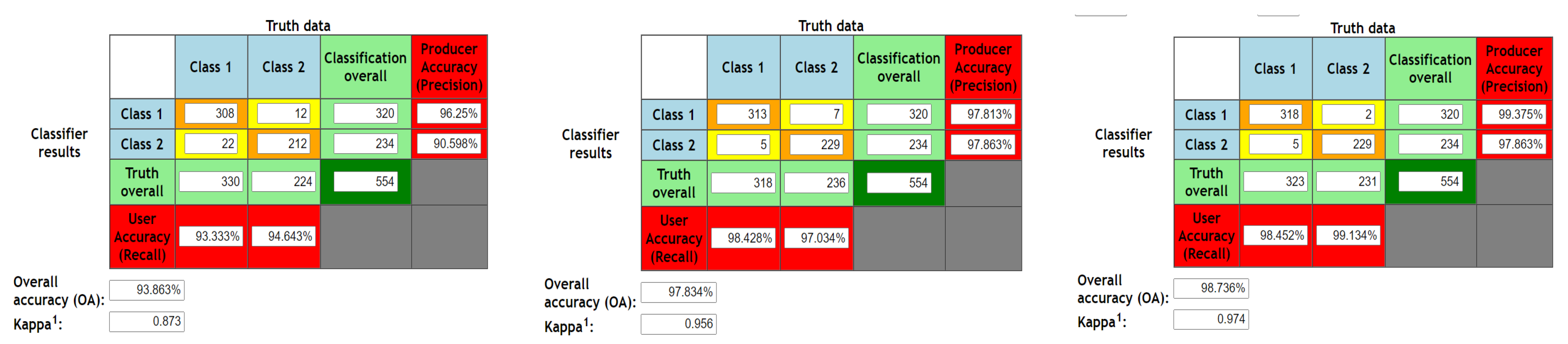
Electronics 10 00495 g008
Figure 9. Confusion matrix for 2 fold cross validation of 2D images for SVM, LSTM and VAE-CNN respectively.
Electronics 10 00495 g009
Figure 10. Confusion matrix for 5 fold cross validation of 2D images for SVM, LSTM and VAE-CNN respectively.
Electronics 10 00495 g010
Figure 11. Confusion matrix for 10 fold cross validation of 2D images for SVM, LSTM and VAE-CNN respectively.
Electronics 10 00495 g011
Figure 12. Confusion matrix for 2 fold cross validation of 3D Doppler images for SVM, LSTM and VAE-CNN respectively.
Electronics 10 00495 g012
Figure 13. Confusion matrix for 5 fold cross validation of 3D Doppler images for SVM, LSTM and VAE-CNN respectively.
Electronics 10 00495 g013
Figure 14. Confusion matrix for 10 fold cross validation of 3D Doppler images for SVM, LSTM and VAE-CNN respectively.
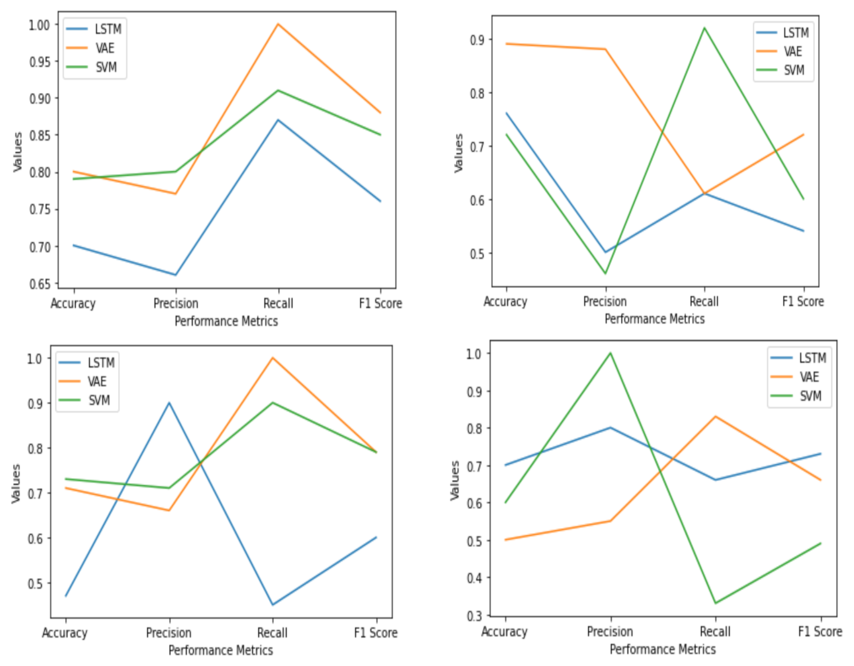
Electronics 10 00495 g014
Figure 15. Graph plotted for validation phase of 2D image and color doppler and testing phase of 2D image and color doppler respectively, without k fold cross validation.
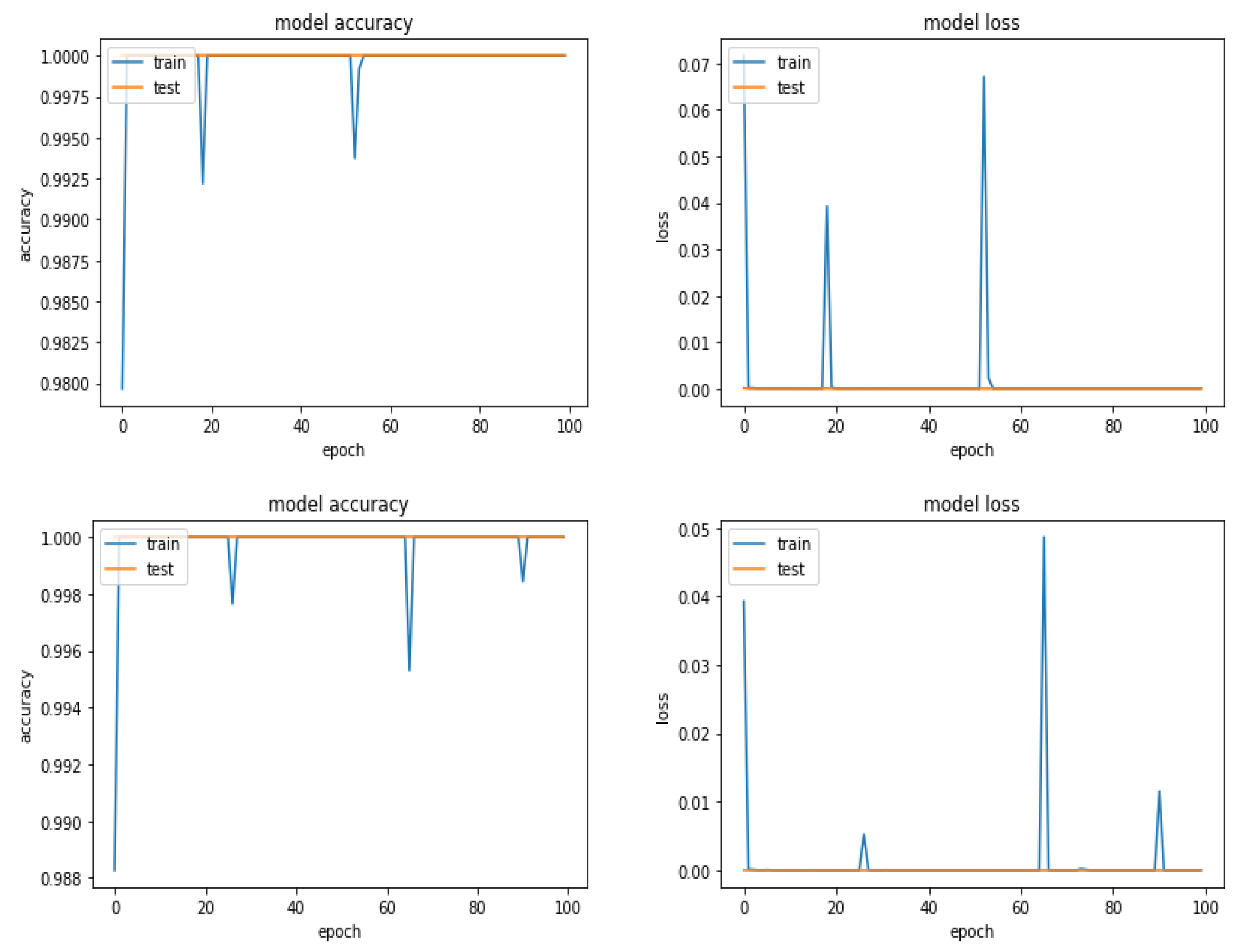
Electronics 10 00495 g015
Figure 16. Accuracy and Loss for LSTM and VAE-CNN for two-class classification for training and validation phase respectively.
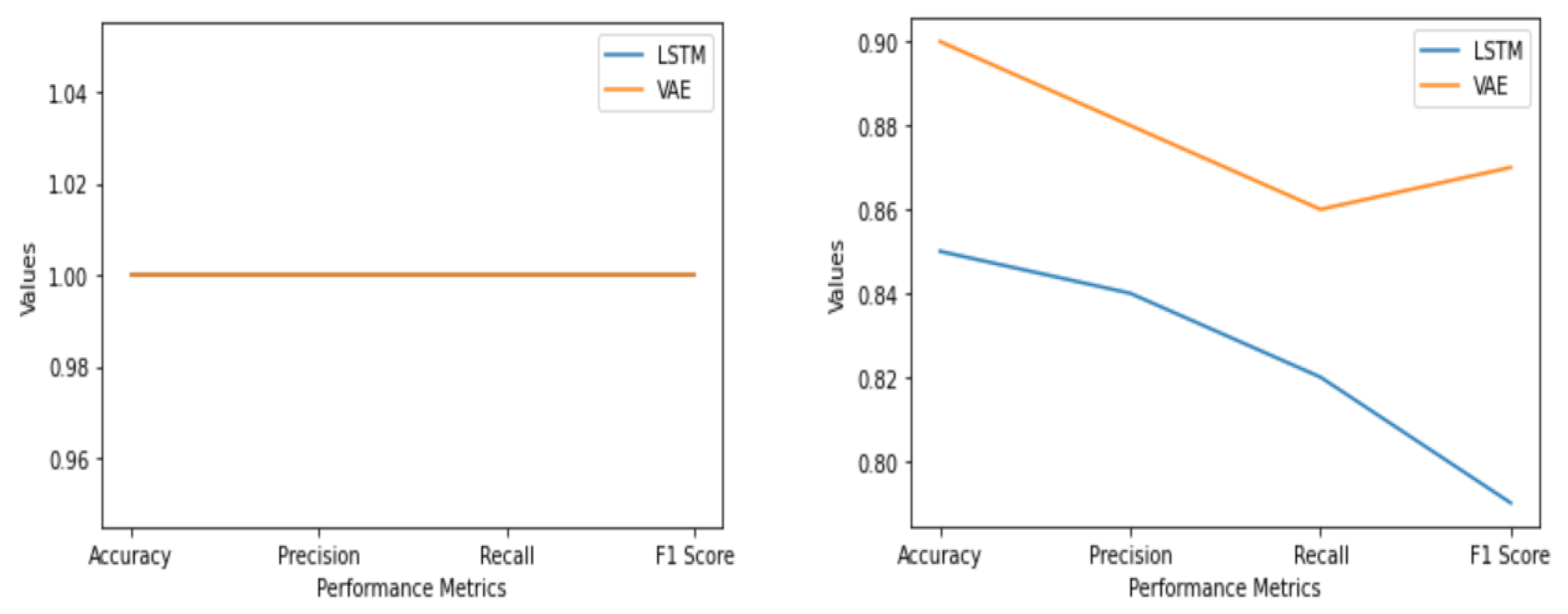
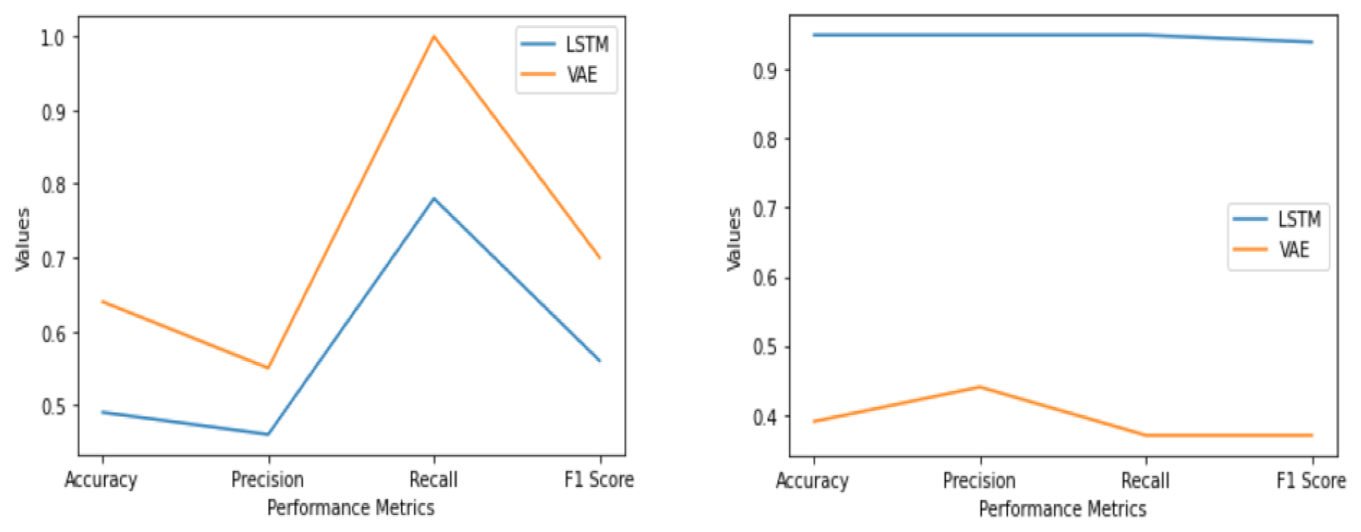
Electronics 10 00495 g016
Figure 17. Validation phase for two-class and six-class and testing phase for two-class and six-class respectively.
Electronics 10 00495 g017aElectronics 10 00495 g017b
Figure 18. Confusion matrix for 2-fold, 5-fold and 10-fold cross validation for LSTM and VAE-CNN, respectively.
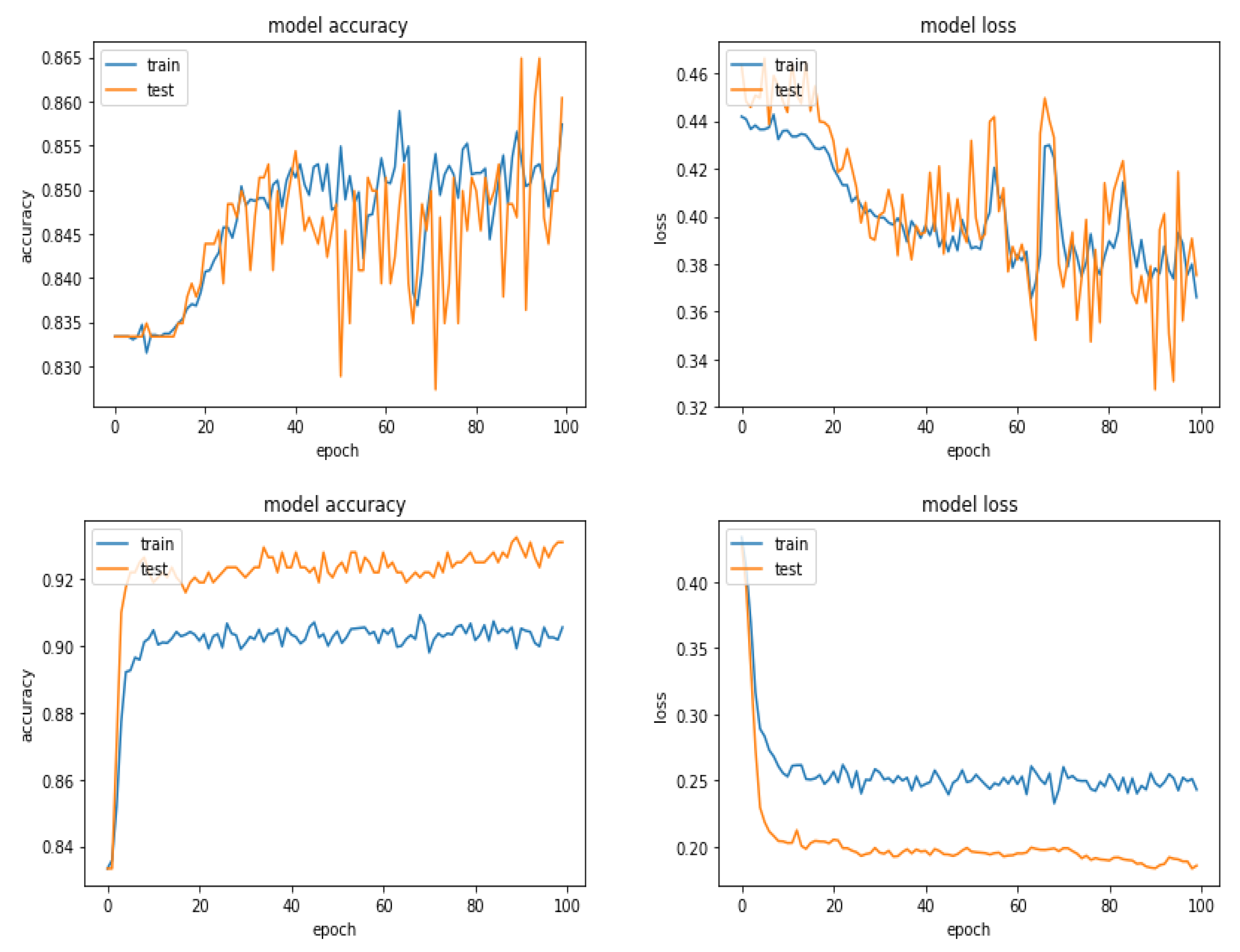
Electronics 10 00495 g018
Figure 19. Accuracy and Loss for LSTM and VAE-CNN for six-class classification for training and validation phase, respectively.
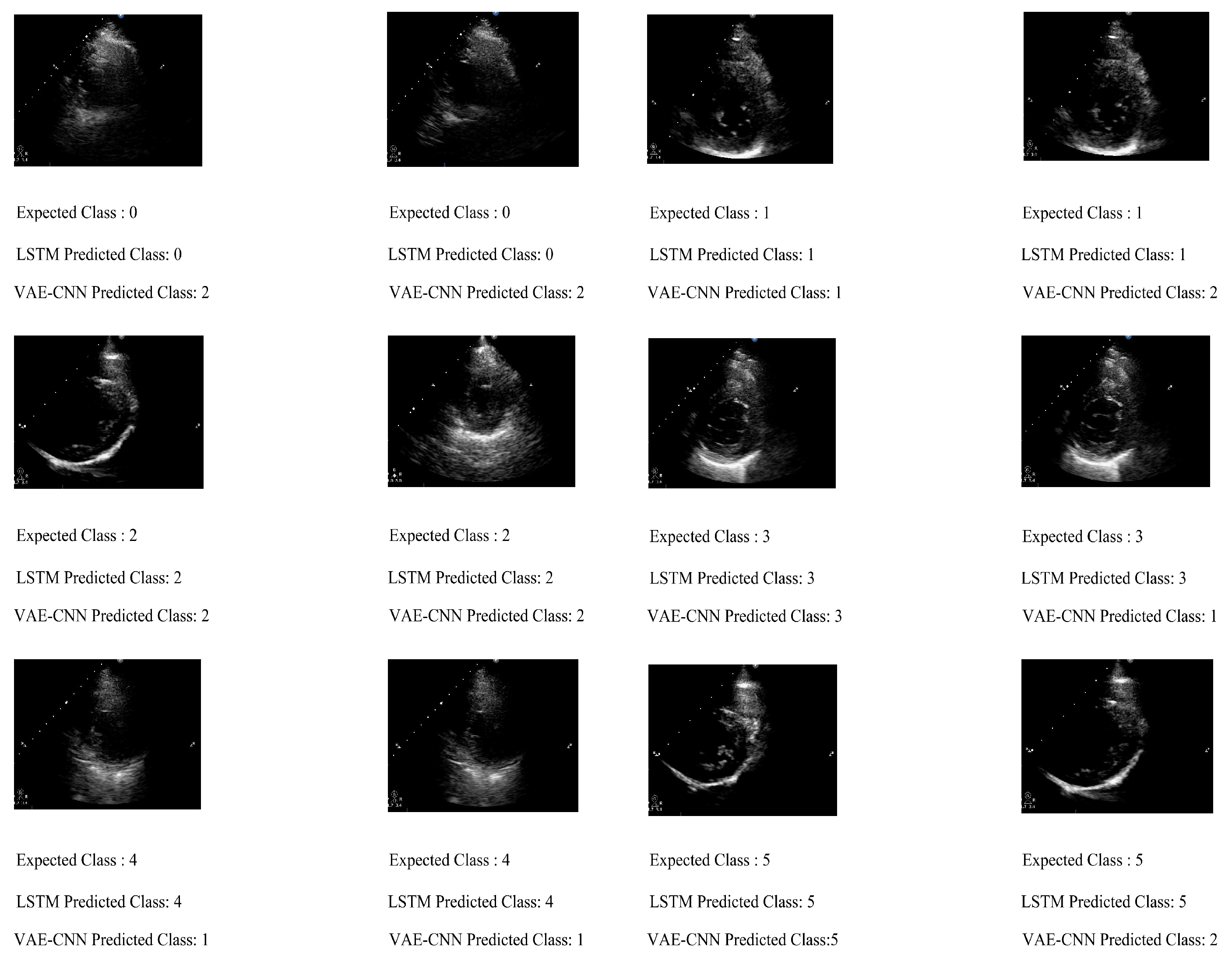
Electronics 10 00495 g019
Figure 20. Output of expected and predicted class for six-class classification using generaliza-tion approach.
Electronics 10 00495 g020
Table 1. Architecture for LSTM and VAE-CNN.
MethodLayer NumberLayer NameLayer Properties
LSTM1Input layerSize 224 × 224
2Covolutional layer 3 × 3 filter size, stride = 2, output size= 115 × 115
3Flatten36,963
4LSTM model126 units
5Dropout50 % dropout
6Fully connected layer50
7Rectified Linear unitsRectified Linear Units
8Sigmoid/SoftmaxSigmoid/Softmax
9Classification output2 (normal or abnormal) and 6 (types of regurgitations)
VAE-CNN1Input image 224 × 224
2Convolutional layer 3 × 3 filter size, stride = 2
3Rectified Linear UnitsRectified Linear Units
4Dropout50 % dropout rate
5Max poolingstride = 2, output size = 115 × 115
6Dropout50 % dropout rate
7Fully Connected9075
8Fully Connected500
9Fully Connected100
10Fully ConnectedSample vector, 30 (Standard deviation), 30 (Mean)
11Fully Connected30
12Sigmoid/SoftmaxSigmoid/Softmax
13Classification layer2 (normal or abnormal) and 6 (types of regurgitations)
Table 2. Output for 2D images and 3D Doppler images.
Echo Format3D Doppler Images2D Images
MethodologiesLSTMVAE-CNNSVMLSTMVAE-CNNSVM
Training Accuracy0.940.960.770.6410.80
Validation (labelled data)Accuracy0.760.890.720.700.800.79
Precision0.500.880.460.660.770.80
Recall0.610.610.920.8710.91
F1 Score0.540.720.600.760.880.85
Testing (unlabelled)Accuracy0.700.500.600.470.710.73
Precision0.800.5510.900.660.71
Recall0.660.830.330.4510.90
F1 Score0.730.660.490.600.790.79
Testing 2 foldAccuracy0.800.940.840.970.980.94
Precision0.920.970.920.970.990.96
Recall0.780.940.830.980.980.93
F1 Score0.840.950.870.970.980.94
Testing 5 foldAccuracy0.720.910.760.920.990.96
Precision0.710.880.730.950.980.97
Recall0.870.960.900.920.980.94
F1 Score0.780.910.800.930.980.98
Testing 10 foldAccuracy0.540.920.760.980.980.98
Precision0.650.940.800.960.980.98
Recall0.600.910.82110.98
F1 Score0.620.920.800.970.980.98
Table 3. Statistical test for comparing methodologies without k fold cross validation.
Type of ImageMethodsPaired T-Test (Validation)Paired T-Test (Testing)
2D imageSVM vs. LSTM0.4930.00014
SVM vs. VAE-CNN0.0420.153
3D Color DopplerSVM vs. LSTM0.0480.0005
SVM vs. VAE-CNN0.00030.0005
Table 4. Confusion matrix for two-class (normal or abnormal) classification.
MethodologiesLSTMVAE-CNN
0101
Validation phase013201320
101110111
Testing phase0191522430
122076191105
Testing 2 fold081208057
106725667
Testing 5 fold032303212
102701269
Testing 10 fold018201811
101142112
Table 5. Confusion matrix for validation and testing into six-class (type of regurgitation) classification.
MethodologiesLSTMVAE-CNN
012345012345
Validation Phase073305007700400
158338000901800
2048090001182000
342374000067700
4304106206243640
5136600560868059
Testing Phase0894030020967000
13178215045802230102
2001340001510951400
300012600048056220
400212870060012290
500000910233615017
Table 6. Output for Video 2 (normal or abnormal) and six-class (types of regurgitation).
Echo FormatVideo 2 ClassVideo 6 Class
MethodologiesLSTMVAE-CNNLSTMVAE-CNN
Training Accuracy110.860.93
ValidationAccuracy110.850.90
Precision110.840.88
Recall110.820.86
F1 Score110.790.87
TestingAccuracy0.490.640.950.39
Precision0.460.550.950.44
Recall0.7810.950.37
F1 Score0.560.700.940.37
Testing 2 foldAccuracy10.990.880.85
Precision10.990.890.85
Recall10.990.890.88
F1 Score10.990.890.86
Testing 5 foldAccuracy10.990.870.85
Precision10.990.860.86
Recall10.990.890.87
F1 Score10.990.870.86
Testing 10 foldAccuracy10.980.890.86
Precision10.980.890.86
Recall10.980.890.89
F1 Score10.980.890.87
Table 7. LSTM precision, recall and F1 Score for validation and testing phase for six-class classification.
NoPrecisionValidationTestingRecallValidationTestingF1 ScoreValidationTesting
1P00.740.96R00.900.92F00.700.93
2P10.820.97R10.830.94F10.820.95
3P20.830.97R20.861F20.840.98
4P30.690.88R30.891F30.770.93
5P410.95R40.780.86F40.870.90
6P511R50.661F50.791
Table 8. VAE-CNN precision, recall and F1 Score for validation and testing phase for six-class classification.
NoPrecisionValidationTestingRecallValidationTestingF1 ScoreValidationTesting
1P00.920.25R00.950.20F00.940.22
2P10.810.34R10.900.42F10.850.36
3P20.820.43R20.880.70F20.840.53
4P30.770.44R30.920.44F30.890.44
5P410.47R40.810.28F40.890.37
6P510.89R50.720.18F50.840.30
Publisher’s Note: MDPI stays neutral with regard to jurisdictional claims in published maps and institutional affiliations.

