A Comparative Analysis of Object Detection Metrics with a Companion Open-Source Toolkit

Abstract

Recent outstanding results of supervised object detection in competitions and challenges are often associated with specific metrics and datasets. The evaluation of such methods applied in different contexts have increased the demand for annotated datasets. Annotation tools represent the location and size of objects in distinct formats, leading to a lack of consensus on the representation. Such a scenario often complicates the comparison of object detection methods. This work alleviates this problem along the following lines: (i) It provides an overview of the most relevant evaluation methods used in object detection competitions, highlighting their peculiarities, differences, and advantages; (ii) it examines the most used annotation formats, showing how different implementations may influence the assessment results; and (iii) it provides a novel open-source toolkit supporting different annotation formats and 15 performance metrics, making it easy for researchers to evaluate the performance of their detection algorithms in most known datasets. In addition, this work proposes a new metric, also included in the toolkit, for evaluating object detection in videos that is based on the spatio-temporal overlap between the ground-truth and detected bounding boxes.

1. Introduction

The human visual system can effectively distinguish objects in different environments and contexts, even under a variety of constraints such as low illumination [1], color differences [2], and occlusions [3,4]. In addition, objects are key to the understanding of a scene’s context, which lends paramount importance to the estimation of their precise location and classification. This has led computer vision researchers to explore automatic object detection for decades [5], reaching impressive results particularly in the last few years [6,7,8,9].

Object detection algorithms attempt to locate general occurrences of one or more predefined classes of objects. In a system designed to detect pedestrians, for instance, an algorithm tries to locate all pedestrians that appear within an image or a video [3,10,11]. In the identification task, however, an algorithm tries to recognize a specific instance of a given class of objects. In the pedestrian example, an identification algorithm wants to determine the identity of each pedestrian previously detected.

Initially, real-time object detection applications were limited to only one object type [12] at a time, mostly due to hardware limitations. Later on, advancements in object detection techniques led to their increasing adoption in areas that included the manufacturing industry with optical inspections [13], video surveillance [14], forensics [15,16], medical image analysis [17,18,19], autonomous vehicles [20], and traffic monitoring [21]. In the last decade, the use of deep neural networks (DNNs) has completely changed the landscape of the computer vision field [22]. DNNs have allowed for drastic improvements in image classification, image segmentation, anomaly detection, optical character recognition (OCR), action recognition, image generation, and object detection [5].

The field of object detection has yielded significant improvements in both efficiency and accuracy. To validate such improvements, new techniques must be assessed against current state-of-the-art approaches, preferably over widely available datasets. However, benchmark datasets and evaluation metrics differ from work to work, often making their comparative assessment confusing and misleading. We identified two main reasons for such confusion in comparative assessments:

• There are often differences in bounding box representation formats among different detectors. Boxes could be represented, for instance by their upper-left corner coordinates (x, y) and their absolute dimensions (width, height) in pixels, or by their relative coordinates ($x_{\mathrm{rel}}$, $y_{\mathrm{rel}}$) and dimensions $({\mathrm{width}}_{\mathrm{rel}},{\mathrm{height}}_{\mathrm{rel}})$, with the values normalized by the image size, among others;
• Each performance assessment tool implements a set of different metrics, requiring specific formats for the ground-truth and detected bounding boxes.

Even though many tools have been developed to convert the annotated boxes from one format to another, the quality assessment of the final detections still lacks a tool compatible with different bounding box formats and multiple metrics. Our previous work [23] contributed to the research community in this direction, by presenting a tool which reads ground-truth and detected bounding boxes in a closed format and evaluates the detections using the average precision (AP) and mean average precision (mAP) metrics, as required in the PASCAL Challenge [24]. In this work that contribution is significantly expanded by incorporating 13 other metrics, as well as by supporting additional annotation formats into the developed open-source toolbox. The new evaluation tool is available at https://github.com/rafaelpadilla/review_object_detection_metrics. We believe that our work significantly simplifies the task of evaluating object detection algorithms.

This work intends to explain in detail the computation of the most popular metrics used as benchmarks by the research community, particularly in online challenges and competitions, providing their mathematical foundations and a practical example to illustrate their applicability. In order to do so, after a brief contextualization of the object-detection field in Section 2, the most common annotation formats and assessment metrics are examined in Section 3 and Section 4, respectively. A numerical example is provided in Section 5 illustrating the previous concepts from a practical perspective. Popular metrics are further addressed in Section 6. In Section 7 object detection in videos is discussed from an integrated spatio-temporal point of view, and a new metric for videos is provided. Section 8 presents an open-source and freely distributed toolkit that implements all discussed concepts in a unified and validated way, as verified in Section 9. Finally, Section 10 concludes the paper by summarizing its main technical contributions.

2. An Overview of Selected Works on Object Detection

Back in the mid-50s and 60s the first attempts to recognize simple patterns in images were published [25,26]. These works identified primitive shapes and convex polygons based on contours. In the mid-80s, more complex shapes started gaining meaning, such as in [27], which described an automated process to construct a three-dimensional geometric description of an airplane.

To describe more complex objects, instead of characterizing them by their shapes, automated feature extraction methods were developed. Different methods attempted to find important feature points that when combined could describe objects broadly. Robust feature points are represented by distinctive pixels, whose neighborhood describe the same object irrespective of changes in pose, rotation, and illumination. The Harris detector [28] finds such points in the object corners based on local intensity changes. A local search algorithm using gradients was devised in [29] to solve the image registration problem, which later was expanded to a tracking algorithm [30] for identifying important points in videos.

More robust methods were able to identify characteristic pixel points and represent them as feature vectors. The so-called scale invariant feature transform (SIFT) [31], for instance, applied the difference of Gaussians in several scales coupled with histograms of gradients, yielding characteristic points with features that are robust to scale changes and rotation. Another popular feature detector and descriptor, the speed up robust features (SURF) [32], was claimed to be faster and more robust than SIFT, and uses a blob detector based on the Hessian matrix for interest point detection and wavelet responses for feature representations.

Feature-point representation methods alone are not able to perform object detection, but can help in extracting a group of keypoints that are used to represent them. In [33], the SIFT keypoints and features are used to detect humans in images, and in [34] SIFT was combined with color histograms to classify regions of interest across frames to track objects in videos. Another powerful feature extractor widely applied for object detection is the histogram of oriented gradients (HOG) [35], which is computed for several image small cells. The histograms of each cell are combined to form the object descriptor, which, associated to a classifier, can perform the object detection task [35,36].

The Viola–Jones object detection framework was described in the path-breaking work of [12]. It could detect a single class object at a rate of 15 frames per second. The proposed algorithm employed a cascade of weak classifiers to process image patches of different sizes, being able to associate bounding boxes to the target object. The Viola–Jones method was first applied to face detection and required extensive training to automatically select a group of Haar-features to represent the target object, thus detecting one class of objects at a time. This framework has been extended to detect other object classes such as pedestrians [10,11] and cars [37].

More recently, with the growth and popularization of deep learning in computer vision problems [6,7,38,39,40], object detection algorithms have started to develop from a new perspective [41,42]. The traditional feature extraction [31,32,35] phase is performed by convolutional neural networks (CNNs), which are dominating computer vision research in many fields. Due to their spatial invariance, convolutions perform feature extraction spatially and can be combined into layers to produce the desired feature maps. The network end is usually composed of fully connected (FC) layers that can perform classification and regression tasks. The output is then compared to a desired result and the network parameters are adjusted to minimize a given loss function. The advantage of using DNNs in object detection tasks is the fact that their architectures can extract features and predict bounding boxes in the same pipeline, allowing efficient end-to-end training. The more layers a network has, the more complex features it is able to extract, but the more parameters it needs to learn, demanding more computer processing power and data.

When it is not feasible to acquire more real data, data augmentation techniques are used to generate artificial but realistic data. Color and geometric operations and changes inside the target object area are the main actions performed by data augmentation methods for object detection tasks [43]. The work in [44] applied generative adversarial networks (GANs) to increase by 10 times the amount of medical chest images to detect patients with COVID-19. In [45], the number of images was increased by applying filters in astronomy images so as to improve the performance of galaxy detectors.

The CNN-based object detectors may be cataloged as single-shot or region-based detectors, also known as one- or two-stage detectors, respectively. The single-shot detectors work by splitting the images into a grid of cells. For each cell, they make bounding-box guesses of different scales and aspect ratios. This type of detector prioritizes speed rather than accuracy, aiming to predict both bounding box and class simultaneously. Overfeat [46] was one of the first single-shot detectors, followed by the single shot multiBox detector (SSD) [47], and all versions of you only look once (YOLO) [9,48,49,50,51]. The region-based detectors perform the detection in two steps. First, they generate a sparse set of region proposals in the image where the objects are supposed to be. The second stage classifies each object proposal and refines its estimated position. The region-based convolutional neural network (R-CNN) [52] was a pioneer employing CNNs in this last stage, achieving significant gains in accuracy. Later works such as Fast R-CNN [53], Faster R-CNN [8], and region-based fully convolutional networks (R-FCN) [54] suggest changes in R-CNN to improve its speed. The aforementioned detectors have some heuristic and hand-crafted steps such as region feature extraction or non-maximum suppression to remove duplicate detections. In this context, graph neural networks (GNNs) are employed to compute region of interest features in a more efficient way and process the objects simultaneously by modeling them according to their appearance feature and geometry [55,56].

Hybrid solutions combining different approaches have been proposed lately and have proved to be more robust in various object-detection applications. The work in [57] proposes a hybrid solution involving a genetic algorithm and CNNs to classify small objects (structures) presented in microscopy images. Feature descriptors coupled with a cuckoo search algorithm were applied by the authors of [58] to detect vessels in a marine environment using synthetic aperture radar (SAR) images. This approach was compared to genetic algorithms and neural network models individually, improving precision to nearly 96.2%. Vision-based autonomous vehicles can also benefit from hybrid models as shown in [59], where a system integrating different approaches was developed to detect and identify pedestrians and to predict their movements. In the context of detecting objects using depth information, the work in [60] proposes a hybrid attention neural network that incorporates depth and high-level RGB features to produce an attention map to remove background information.

Other works aim to detect the most important region of interest and segment relevant objects using salient object detectors. The work in [61] proposes a pipeline to separate an input image into a pair of images using content-preserving transforms. Then, each resulting image is passed by an interweaved convolutional neural network, which extracts complementary information of the image pairs and fuses them into the final salient map.

As medical images are acquired with special equipment, they form a very specific type of image [17]. To detect lesions, organs, and other structures of interest can be crucial for a precise diagnostic. However, most object detection systems are designed for general applications and usually do not perform well in medical images without adaptations [62]. Detecting anomalies such as glaucoma, breast, and lung lesions, for instance, have been explored from the medical object-detection perspective in [63,64]. In the medical field, training and testing data usually have significant differences due to data scarcity and privacy. In order to address this issue, a domain adaptation framework, referred to as clustering CNNs (CLU-CNNs) [65], has been proposed to improve the generalization capability without specific domain training.

With new object detection methods being constantly released, it is highly desirable that a consensual evaluation procedure is established. To do so, the most common bounding box formats used by public datasets and competitions are revised in the next section.

3. Bounding Box Formats

Given the large, ever growing number of object detectors based on supervised methods in different areas, specific datasets have been built to train these systems. Popular competitions such as the common objects in context (COCO) [66], PASCAL visual object classes (VOC) [67], and Open Images Dataset [68] offer annotated datasets so that participants can train and evaluate their models before submission. Apart from using available datasets, collecting data for a object detection task can be quite challenging, as labeling images and videos is often a manual and quite demanding exercise. The medical field provides a good example of this fact: Developing a database of X-ray, electroencephalography (EEG), magnetoencephalography (MEG), or electrocardiography (ECG) images involves not only high costs for capturing such signals, but also requires expert knowledge to interpret and annotate them.

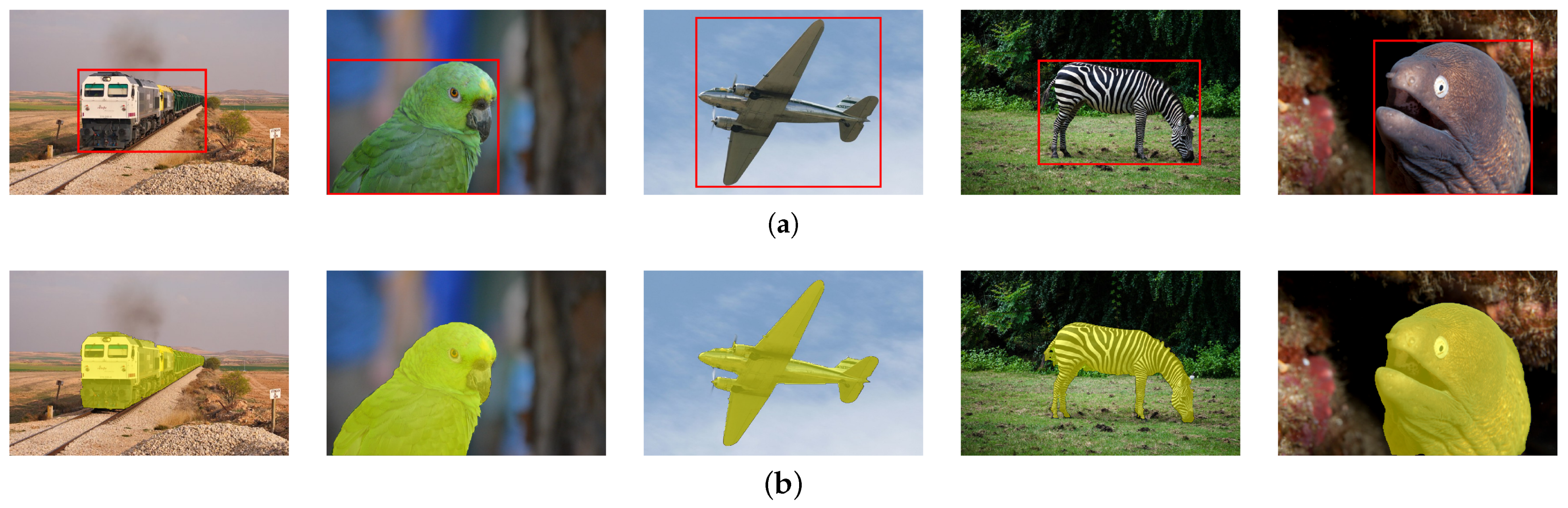
To ease the object annotation process in images and videos, many tools have been developed to annotate different datasets. Such tools basically offer the same features, such as bounding-box annotations and polygon-like silhouettes, as shown in Figure 1.

A vast amount of annotation tools are freely available.

Table 1. Popular free annotation tools and their supported output formats.

Annotation Tool	Annotation Types	Output Formats
LabelMe [69]	Bounding boxes and polygons	LabelMe, but provides conversion to COCO and PASCAL VOC
LabelIMG [70]	Bounding boxes	PASCAL VOC and YOLO
Microsoft VoTT [71]	Bounding boxes and polygons	PASCAL VOC, TFRecords, specific CSV, Azure Custom Vision Service, Microsoft Cognitive Toolkit (CNTK), VoTT
Computer Vision Annotation Tool (CVAT) [72]	Bounding boxes and polygons	COCO, CVAT, LabelMe, PASCAL VOC, TFRecord, YOLO, and others
VGG Image Annotation Tool (VIA) [73]	Bounding boxes and polygons	COCO and specific CSV and JSON

lists the most popular ones with their respective bounding box output formats.

Some datasets introduced new formats to represent their annotations, which are usually named after the datasets themselves. The PASCAL VOC dataset [67] established the PASCAL VOC XML format and the COCO dataset [66] represents their annotations in the COCO format, embodied in a JSON file. Annotation tools also brought further formats. For example, CVAT [72], a popular annotation tool, outputs bounding boxes in multiple formats, including its own specific XML-based one, named a CVAT format. The most popular bounding box formats shown in Table 1 are described in more detail. Note that whenever we refer to absolute coordinates, we mean coordinates that are expressed on the image coordinate frame, as opposed to coordinates that are normalized by the image width or image height.

• PASCAL VOC: It consists of one XML file for each image containing none, one or multiple bounding boxes. The upper-left and bottom-right pixel coordinates are absolute. Each bounding box also contains a tag representing the class of the object. Extra information about the labeled object can be provided, such as whether, the object extends beyond the bounding box or it is partially occluded. The annotations in the ImageNet [74] and PASCAL VOC [67] datasets are provided using the PASCAL VOC format;
• COCO: It is represented by a single JSON file containing all bounding boxes of a given dataset. The classes of the objects are listed separately in the categories tag and identified by an id. The image file corresponding to an annotation is also indicated in a separate element (images) that contains its file name and is referenced by an id. The bounding boxes and their object classes are listed in a different element (annotations), with their top-left $(x,y)$ coordinates being absolute, and with explicit values of width and height;
• LabelMe: The bounding-box annotations in this format are inserted in a single JSON file for each image, containing a list of boxes represented by their absolute upper-left and bottom-right coordinates. Besides the class of the object, this format also contains the image data encoded in base64 type, thus making the LabelMe format to consume more storage space than others;
• YOLO: One TXT file per image is used in this representation. Each line of the file contains the class id and the bounding box coordinates. An extra file is needed to map the class id to the class name. The bounding box coordinates are not absolute, being represented by the format ($\frac{x_{\mathrm{center}}}{\mathrm{image}\mathrm{width}},\frac{y_{\mathrm{center}}}{\mathrm{image}\mathrm{height}},\frac{\mathrm{box}\mathrm{width}}{\mathrm{image}\mathrm{width}},\frac{\mathrm{height}}{\mathrm{image}\mathrm{height}}$). The advantage of representing the boxes in this format is that, if the image dimensions are scaled, the bounding box coordinates do not change, and thus the annotation file does not have to be altered. This type of format is the one preferred by those who annotate images in one resolution and need to scale their dimensions to fulfill the input shape requirement of a specific CNN. The YOLO object detector needs bounding boxes in this format to execute training;
• VoTT: This representation of the bounding boxes coordinates and object class is made in a JSON file (one file per image) and the coordinates are expressed as the width, height and upper-left $(x,y)$ pixel position in absolute coordinates. The Visual Object Tagging Tool (VoTT) produces annotations in this format;
• CVAT: It consists of a unique XML file with all bounding boxes in the dataset represented by the upper-left and bottom-right pixel absolute coordinates. This format has been created with the CVAT annotation tool;
• TFRecord: This is a serialized representation of the whole dataset containing all images and annotations in a single file. This format is recognized by the Tensorflow library [75];
• Tensorflow Object Detection: This is a CSV file containing all labeled bounding boxes of the dataset. The bounding box format is represented by the upper-left and bottom-right pixel absolute coordinates. This is also a widely used format employed by the Tensorflow library;
• Open Images Dataset: This format is associated with the Open Images Dataset [68] to annotate its ground-truth bounding boxes. All annotations are written in a unique CSV file listing the name of the images and labels, as well as upper-left and bottom-right absolute coordinates of the bounding boxes. Extra information about the labeled object is conveyed by other tags such as, for example, IsOcclude, IsGroupOf, and IsTruncated.

As each dataset is annotated using a specific format, works tend to employ the evaluation tools provided along with the datasets to assess their performance. Therefore, their results are dependent on the specific metric implementation associated with the used dataset. For example, the PASCAL VOC dataset employs the PASCAL VOC annotation format, which provides a MATLAB code implementing the metrics AP and mAP (intersection over union (IOU)=.50). This tends to inhibit the use of other metrics to report results obtained for this particular dataset.

Table 2. Popular object detection methods along with the datasets and metrics used to report their results.

Method	Benchmark Dataset	Metrics
CornerNet [76]	COCO	AP@[.5:.05:.95]; AP@.50; AP@.75; APS; APM; APL
EfficientDet [77]	COCO	AP@[.5:.05:.95]; AP@.50; AP@.75
Fast R-CNN [53]	PASCAL VOC 2007, 2010, 2012	AP; mAP (IOU=.50)
Faster R-CNN [8]	PASCAL VOC 2007, 2012	AP; mAP (IOU=.50)
Faster R-CNN [8]	COCO	AP@[.5:.05:.95]; AP@.50
R-CNN [52]	PASCAL VOC 2007, 2010, 2012	AP; mAP (IOU=.50)
RFB Net [78]	PASCAL VOC 2007	mAP (IOU=.50)
RFB Net [78]	COCO	AP@[.5:.05:.95]; AP@.50; AP@.75; APS; APM; APL
RefineDet [79]	PASCAL VOC 2007, 2012	mAP (IOU=.50)
RefineDet [79]	COCO	AP@[.5:.05:.95]; AP@.50; AP@.75; APS; APM; APL
RetinaNet [80]	COCO	AP@[.5:.05:.95]; AP@.50; AP@.75; APS; APM; APL
R-FCN [54]	PASCAL VOC 2007, 2012	mAP (IOU=.50)
R-FCN [54]	COCO	AP@[.5:.05:.95];AP@.50; APS; APM; APL
SSD [47]	PASCAL VOC 2007, 2012	mAP (IOU=.50)
SSD [47]	COCO	AP@[.5:.05:.95]; AP@.50; AP@.75; APS; APM; APL; AR1; AR10; AR100; ARS; ARM; ARL
SSD [47]	ImageNet	mAP (IOU=.50)
Yolo v1 [48]	PASCAL VOC 2007, 2012; Picasso; People-Art	AP; mAP (IOU=.50)
Yolo v2 [49]	PASCAL VOC 2007, 2012	AP; mAP (IOU=.50)
Yolo v2 [49]	COCO	AP@[.5:.05:.95]; AP@.50; AP@.75; APS; APM; APL; AR1; AR10; AR100; ARS; ARM; ARL
Yolo v3 [50]	COCO	AP@[.5:.05:.95]; AP@.50; AP@.75; APS; APM; APL; AR1; AR10; AR100; ARS; ARM; ARL
Yolo v4 [51]	COCO	AP@[.5:.05:.95]; AP@.50; AP@.75; APS; APM; APL
Yolo v5 [9]	COCO	AP@[.5:.05:.95]; AP@.50

lists popular object detection methods along with the datasets and the 14 different metrics used to report their results, namely: AP@[.5:.05:.95], AP@.50, AP@.75, AP_S, AP_M, AP_L, AR₁, AR₁₀, AR₁₀₀, AR_S, AR_M, AR_L, mAP (IOU=.50), and AP.

As the evaluation metrics are directly associated with a given annotation format, almost all works report their results only for the metrics implemented for the benchmarking dataset. For example, mAP (IOU=.50) is reported when the PASCAL VOC dataset is used, while AP@[.5:.05:.95] is applied to report results on the COCO dataset. If a work uses the COCO dataset to train a model and wants to evaluate their results with the PASCAL VOC tool, it will be necessary to convert the ground-truth COCO JSON format to the PASCAL VOC XML format. This scenario discourages the use of such cross-dataset assessments, which have become quite rare in the object detection literature.

An example of confusions that may arise in such a scenario is given by the fact that some works affirm that the metrics AP@.50 and mAP (IOU=.50) are the same [54], which may not always be true. The origins of such misunderstandings are the differences in how each tool computes the corresponding metrics. The next section deals with this problem by detailing the implementations of the several object detection metrics and pointing out their differences.

4. Performance Metrics

Challenges and online competitions have pushed forward the frontier of the object detection field, improving results for specific datasets in every new edition. To validate the submitted results, each competition applies a specific metric to rank the submitted detections. These assessment criteria have also been used by the research community to report and compare object detection methods using different datasets as illustrated in Table 2. Among the popular metrics to report the results, this section will cover those used by the most popular competitions, namely Open Images RVC [81], COCO Detection Challenge [82], VOC Challenge [24], Datalab Cup [83], Google AI Open Images challenge [84], Lyft 3D Object Detection for Autonomous Vehicles [85], and City Intelligence Hackathon [86]. Object detectors aim to predict the location of objects of a given class in an image or video with a high confidence. They do so by placing bounding boxes to identify the positions of the objects. Therefore, a detection is represented by a set of three attributes: The object class, the corresponding bounding box, and the confidence score, usually given by a value between 0 and 1 showing how confident the detector is about that prediction. The assessment is done based on:

• A set of ground-truth bounding boxes representing the rectangular areas of an image containing objects of the class to be detected, and
• a set of detections predicted by a model, each one consisting of a bounding box, a class, and a confidence value.

Detection evaluation metrics are used to quantify the performance of detection algorithms in different areas and fields [87,88]. In the case of object detection, the employed evaluation metrics measure how close the detected bounding boxes are to the ground-truth bounding boxes. This measurement is done independently for each object class, by assessing the amount of overlap of the predicted and ground-truth areas.

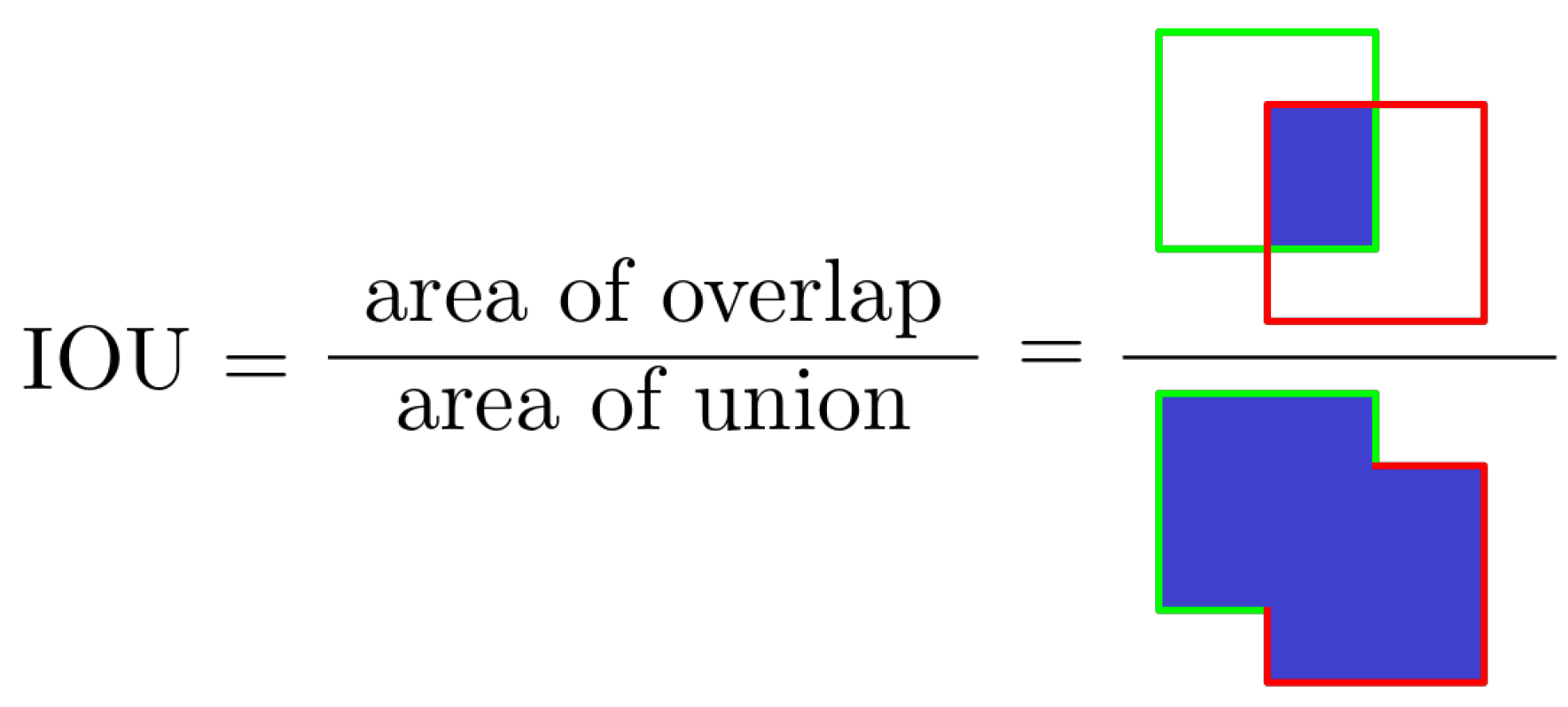
Consider a target object to be detected represented by a ground-truth bounding box $B_{gt}$ and the detected area represented by a predicted bounding box $B_p$. Without taking into account a confidence level, a perfect match is considered when the area and location of the predicted and ground-truth boxes are the same. These two conditions are assessed by the intersection over union (IOU), a measurement based on the Jaccard Index, a coefficient of similarity for two sets of data [89]. In the object detection scope, the IOU is equal to the area of the overlap (intersection) between the predicted bounding box $B_{\mathit{p}}$ and the ground-truth bounding box $B_{\mathit{gt}}$ divided by the area of their union, that is:

$$J(B_p,B_{\mathit{gt}})=\mathrm{IOU}=\frac{\mathrm{area}(B_p\cap B_{\mathit{gt}})}{\mathrm{area}(B_p\cup B_{\mathit{gt}})},$$

(1)

as illustrated in Figure 2.

A perfect match occurs when $\mathrm{IOU}=1$ and, if both bounding boxes do not intercept each other, $\mathrm{IOU}=0$. The closer to 1 the IOU gets, the better the detection is considered. As object detectors also perform the classification of each bounding box, only ground-truth and detected boxes of the same class are comparable through the IOU.

By setting an IOU threshold, a metric can be more or less restrictive on considering detections as correct or incorrect. An IOU threshold closer to 1 is more restrictive as it requires almost-perfect detections, while an IOU threshold closer to, but different than 0 is more flexible, considering as detections even small overlaps between $B_p$ and $B_{gt}$. IOU values are usually expressed in percentages, and the most used threshold values are $50\%$ and $75\%$. In Section 4.1, Section 4.2, and Section 4.4 the IOU is used to define the metrics that are most relevant to object detection.

4.1. Precision and Recall

Let us consider a detector that assumes that every possible rectangular region of the image contains a target object (this would be done by placing bounding boxes of all possible sizes centered in every image pixel). If there is one object to be detected, the detector would correctly find it by one of the many predicted bounding boxes. That is not an efficient way to detect objects, as many wrong predictions are made as well. Conversely, a detector which never generates any bounding box, will never have a miss-detection. These extreme examples highlight two important concepts, referred as precision and recall, are further explained below.

Precision is the ability of a model to identify only relevant objects. It is the percentage of correct positive predictions. Recall is the ability of a model to find all relevant cases (all ground-truth bounding boxes). It is the percentage of correct positive predictions among all given ground truths. To calculate the precision and recall values, each detected bounding box must first be classified as:

• True positive (TP): A correct detection of a ground-truth bounding box;
• False positive (FP): An incorrect detection of a non-existing object or a misplaced detection of an existing object;
• False negative (FN): An undetected ground-truth bounding box.

Assuming there is a dataset with G ground-truths and a model that outputs N detections, of which S are correct ($S\le G$), the concepts of precision and recall can be formally expressed as:

$$\begin{array}{ccc}\hfill \mathit{Pr}& =& \frac{{\displaystyle \sum _{n=1}^S{\mathrm{TP}}_n}}{{\displaystyle \sum _{n=1}^S{\mathrm{TP}}_n+\sum _{n=1}^{N-S}{\mathrm{FP}}_n}}=\frac{{\displaystyle \sum _{n=1}^S{\mathrm{TP}}_n}}{\mathrm{all}\mathrm{detections}},\hfill \end{array}$$

(2)

$$\begin{array}{ccc}\hfill \mathit{Rc}& =& \frac{{\displaystyle \sum _{n=1}^S{\mathrm{TP}}_n}}{{\displaystyle \sum _{n=1}^S{\mathrm{TP}}_n+\sum _{n=1}^{G-S}{\mathrm{FN}}_n}}=\frac{{\displaystyle \sum _{n=1}^S{\mathrm{TP}}_n}}{\mathrm{all}\mathrm{ground}\mathrm{truths}}.\hfill \end{array}$$

(3)

4.2. Average Precision

As discussed above, the output of an object detector is characterized by a bounding box, a class, and a confidence interval. The confidence level can be taken into account in the precision and recall calculations by considering as positive detections only those whose confidence is larger than a confidence threshold $\tau$. The detections whose confidence level is smaller than $\tau$ are considered as negatives. By doing so, one may rewrite Equations (2) and (3) to consider this dependence on the confidence threshold $\tau$ as:

$$\begin{array}{ccc}\hfill \mathit{Pr}\left(\tau \right)& =& \frac{{\displaystyle \sum _{n=1}^S{\mathrm{TP}}_n\left(\tau \right)}}{{\displaystyle \sum _{n=1}^S{\mathrm{TP}}_n\left(\tau \right)+\sum _{n=1}^{N-S}{\mathrm{FP}}_n\left(\tau \right)}}=\frac{{\displaystyle \sum _{n=1}^S{\mathrm{TP}}_n\left(\tau \right)}}{\mathrm{all}\mathrm{detections}\left(\tau \right)},\hfill \end{array}$$

(4)

$$\begin{array}{ccc}\hfill \mathit{Rc}\left(\tau \right)& =& \frac{{\displaystyle \sum _{n=1}^S{\mathrm{TP}}_n\left(\tau \right)}}{{\displaystyle \sum _{n=1}^S{\mathrm{TP}}_n\left(\tau \right)+\sum _{n=1}^{G-S}{\mathrm{FN}}_n\left(\tau \right)}}=\frac{{\displaystyle \sum _{n=1}^S{\mathrm{TP}}_n\left(\tau \right)}}{\mathrm{all}\mathrm{ground}\mathrm{truths}}.\hfill \end{array}$$

(5)

Both TP$\left(\tau \right)$ and FP$\left(\tau \right)$ are decreasing functions of $\tau$, as a larger $\tau$ reduces the number of positive detections. Conversely, FN$\left(\tau \right)$ is an increasing function of $\tau$, since less positive detections imply a larger number of negative detections. In addition, $\sum \mathrm{TP}\left(\tau \right)+\sum \mathrm{FN}\left(\tau \right)$ does not depend on $\tau$ and is a constant equal to the number of all the ground truths. Therefore, from Equation (5), the recall $\mathit{Rc}\left(\tau \right)$ is a decreasing function of $\tau$. On the other hand, nothing can be said a priori about the precision $\mathit{Pr}\left(\tau \right)$, since both the numerator and denominator of Equation (4) are decreasing functions of $\tau$, and indeed the graph of $\mathit{Pr}\left(\tau \right)\times \mathit{Rc}\left(\tau \right)$ tends to exhibit a zig-zag behavior in practical cases, as later illustrated in Section 5.

In practice, a good object detector should find all ground-truth objects ($\mathrm{FN}=0$≡ high recall), while identifying only relevant objects ($\mathrm{FP}=0$≡ high precision). Therefore, a particular object detector can be considered good if, when the confidence threshold decreases, its precision remains high as its recall increases. Hence, a large area under the curve (AUC) tends to indicate both high precision and high recall. Unfortunately, in practical cases, the precision × recall plot is often not monotonic, being zigzag-like instead, which poses challenges to an accurate measurement of its AUC.

The average precision (AP) is a metric based on the area under a $\mathit{Pr}\times \mathit{Rc}$ curve that has been pre-processed to eliminate the zig-zag behavior. It summarizes this precision-recall trade-off dictated by confidence levels of the predicted bounding boxes.

To compute the AP, one starts by ordering the K different confidence values $\tau \left(k\right)$ output by the object detector as:

$$\tau \left(k\right),k=1,2,\dots ,K\mathrm{such}\mathrm{that}\tau \left(i\right)>\tau \left(j\right)\mathrm{for}i>j.$$

(6)

Since the $\mathit{Rc}$ values also have a one-to-one, monotonic correspondence with $\tau$, which has a one-to-one, monotonic, correspondence with the index k, then the $\mathit{Pr}\times \mathit{Rc}$ curve is not continuous but sampled at the discrete points $\mathit{Rc}\left(\tau \right(k\left)\right)$, leading to the set of pairs ($\mathit{Pr}\left(\tau \right(k),\mathit{Rc}(\tau \left(k\right))$ indexed by k.

Now one defines an ordered set of reference recall values $R_r\left(n\right)$,

$$R_r\left(n\right),n=1,2,\dots ,N\mathrm{such}\mathrm{that}{R}_r\left(m\right)<R_r\left(n\right)\mathrm{for}m>n.$$

(7)

The AP is computed using the two ordered sets in Equations (6) and (7). But before computing AP, the precision × recall pairs have to be interpolated such that the resulting precision × recall curve is monotonic. The resulting interpolated curve is defined by a continuous function ${\mathit{Pr}}_{\mathrm{interp}}\left(\mathit{R}\right)$, where $\mathit{R}$ is a real value contained in the interval $[0,1]$, defined as:

$${\mathit{Pr}}_{\mathrm{interp}}\left(\mathit{R}\right)=\underset{k\left|\mathit{Rc}\right(\tau \left(k\right))\ge R}{max}\left\{\mathit{Pr}\left(\tau \left(k\right)\right)\right\},$$

(8)

where $\tau \left(k\right)$ is defined in Equation (6) and $\mathit{Rc}\left(\tau \right(k\left)\right)$ is the recall value for the confidence $\tau \left(k\right)$, computed according to Equation (5). The precision value interpolated at recall R corresponds to the maximum precision ${\mathit{Pr}}_{\mathrm{interp}}\left(k\right)$ whose corresponding recall value is greater than or equal to R. Note that an interpolation using a polynomial fitting would not be convenient in this case, since a polynomial interpolation cannot guarantee that the resulting interpolated curve is monotonic.

Now one is ready to compute AP by sampling ${\mathit{Pr}}_{\mathrm{interp}}\left(\mathit{R}\right)$ at the N reference recall values $R_r$ defined in Equation (7). The AP is the area under the $\mathit{Pr}\times \mathit{Rc}$ curve calculated by a Riemann integral of ${\mathit{Pr}}_{\mathrm{interp}}\left(\mathit{R}\right)$ using the K recall values from the set $R_r\left(k\right)$ in Equation (7) as sampling points, that is,

$$\mathrm{AP}=\sum _{k=0}^K(R_r\left(k\right)-R_r(k+1)){\mathit{Pr}}_{\mathrm{interp}}\left(R_r\left(k\right)\right),$$

(9)

where ${\mathit{Pr}}_{\mathrm{interp}}\left(\mathit{R}\right)$ is defined in Equation (8) and $Rr\left(k\right)$ is given by Equation (12), with $R_r\left(0\right)=1$ and $R_r(K+1)=0$.

There are basically two approaches to compute this Riemann integral: The N-point interpolation and the all-point interpolation, as detailed below.

4.2.1. N-Point Interpolation

In the N-point interpolation, the set of reference recall values $R_r\left(n\right)$ for the computation of the Riemann integral in Equation (9) are equally spaced in the interval $[0,1]$, that is,

$$R_r\left(n\right)=\frac{N-n}{N-1},n=1,2,\dots ,N.$$

(10)

and thus the expression for AP becomes:

$$\mathrm{AP}=\frac{1}{N}\sum _{n=1}^N{\mathit{Pr}}_{\mathrm{interp}}\left(R_r\left(n\right)\right).$$

(11)

Actually the N-point interpolation as defined by Equation (11) computes an AP value which is equal to the value computed by the Riemann integral in Equation (9) multiplied by $\frac{N-1}{N}$.

Popular applications of this interpolation method use $N=101$ as in the competition [82] and $N=11$ as initially adopted by the competition [24], which was later changed to the all-point interpolation method.

4.2.2. All-Point Interpolation

For the computation of AP using the so-called all-point interpolation, here referred to as ${\mathrm{AP}}_{\mathrm{all}}$, as the set values $R_r\left(n\right)$ used to compute the Riemann integral in Equation (9) corresponds exactly to the set of recall values computed considering all K confidence levels $\tau \left(k\right)$ in Equation (6), with the confidences $\tau \left(0\right)=0$ and $\tau (K+1)=1$ added so that the points $R_r\left(0\right)=1$ and $R_r(K+1)=0$ are considered in Equation (9). More precisely,

$$\begin{array}{ccc}\hfill R_r\left(0\right)& =& 1,\hfill \\ \hfill R_r\left(k\right)& =& \mathit{Rc}\left(\tau \right(k\left)\right),k=1,2,\dots ,K,\hfill \\ \hfill R_r(K+1)& =& 0.\hfill \end{array}$$

(12)

where $\mathit{Rc}\left(\tau \right(k\left)\right)$ is given by Equation (5) with $\mathit{Rc}\left(\tau \right(0\left)\right)=1$ and $\mathit{Rc}\left(\tau \right(K+1\left)\right)=0$.

Using this definition of $R_r\left(k\right)$ in Equation (12), ${\mathrm{AP}}_{\mathrm{all}}$ is computed using Equation (9). In the all-point interpolation, instead of using the precision observed at only a few points, the AP is obtained by interpolating the precision at each recall level. The Pascal Challenge [24] adopts the all-point interpolation method to compute the average precision.

4.3. Mean Average Precision

Regardless of the interpolation method, AP is obtained individually for each class. In large datasets with many classes, it is useful to have a unique metric that is able to represent the exactness of the detections among all classes. For such cases, the mean average precision (mAP) is computed, which is simply the average AP over all classes [8,47], that is,

$$\mathrm{mAP}=\frac{1}{C}\sum _{i=1}^C{\mathrm{AP}}_i,$$

(13)

where ${\mathrm{AP}}_i$ is the AP value for the i-th class and C is the total number of classes being evaluated.

4.4. Average Recall

The average recall (AR) [90] is another evaluation metric used to measure the assertiveness of object detectors for a given class. Unlike the average precision, the confidences of the estimated detections are not taken into account in AR computation. This turns all detections into positive ones, which is equivalent to setting the confidence threshold as $\tau =0$ in Equations (4) and (5).

The AR metric makes an evaluation at a large range of IOU thresholds, by taking into account all recall values obtained for IOU thresholds in the interval $[0.5,1]$. An IOU of 0.5 can be interpreted as a rough localization of an object and is the least acceptable IOU by most of the metrics, and an IOU equal to 1 is equivalent to the perfect location of the detected object. Therefore, by averaging recall values in the interval $[0.5,1]$, the model is evaluated on the condition of the object location being considerably accurate.

Let o be the IOU overlap between a ground truth and a detected bounding box as computed by Equation (1), and ${\mathit{Rc}}_{\mathit{IOU}}\left(o\right)$ a function that retrieves the recall for a given IOU o. The AR is defined as twice the area under the ${\mathit{Rc}}_{\mathit{IOU}}\left(o\right)\times o$ curve for the IOU interval $[0.5,1]$, that is,

$$\mathrm{AR}=2{\int }_{0.5}^1{\mathit{Rc}}_{\mathit{IOU}}\left(o\right)do.$$

(14)

The authors in [90] also give a straightforward equation for the computation of the above integral from the discrete sample set, as twice the average of the excess IOU for all the ground-truths, that is,

$$\mathrm{AR}=\frac{2}{G}\sum _{i=1}^{G}max({\mathrm{IOU}}_i-0.5,0),$$

(15)

where ${\mathrm{IOU}}_i$ denotes the best IOU obtained for a given ground truth i and G is the total number of ground-truths.

Interestingly, COCO also reports the AR, although its definition does not match exactly that in Equation (15). Instead, what is reported as the COCO AR is the average of the maximum obtained recall across several IOU thresholds. To do so one first defines a set of O IOU thresholds:

$$t\left(o\right),o=1,2,\dots ,O.$$

(16)

Then, letting ${\mathit{Pr}}_{t\left(o\right)}\left(\tau \left(k\right)\right),{\mathit{Rc}}_{t\left(o\right)}\left(\tau \left(k\right)\right)$ be the precision × recall points for a confidence $\tau \left(k\right)$, given the IOU threshold $t\left(o\right)$, the COCO AR is computed as:

$$\mathrm{AR}=\frac{1}{O}\sum _{o=1}^O\underset{k|{\mathit{Pr}}_{t\left(o\right)}\left(\tau \left(k\right)\right)>0}{max}\left\{{\mathit{Rc}}_{t\left(o\right)}\left(\tau \left(k\right)\right)\right\},$$

(17)

that is, the average of the largest recall values such that the precision is greater than zero for each IOU threshold, and $\tau \left(k\right)$ as defined in Equation (6). Effectively, this yields a coarse approximation of the original integral in Equation (14), provided that the IOU threshold set $t\left(o\right)$ covers an adequate range of overlaps.

4.5. Mean Average Recall

As the AR is calculated individually for each class, similarly to what is done to compute mAP, a unique AR value can be obtained considering the mean AR among all classes, that is:

$$\mathrm{mAR}=\frac{1}{C}\sum _{i=1}^C{\mathrm{AR}}_i.$$

(18)

In the sequel, a practical example illustrates the differences reflected in the final result depending on the chosen method.

5. A Numerical Example

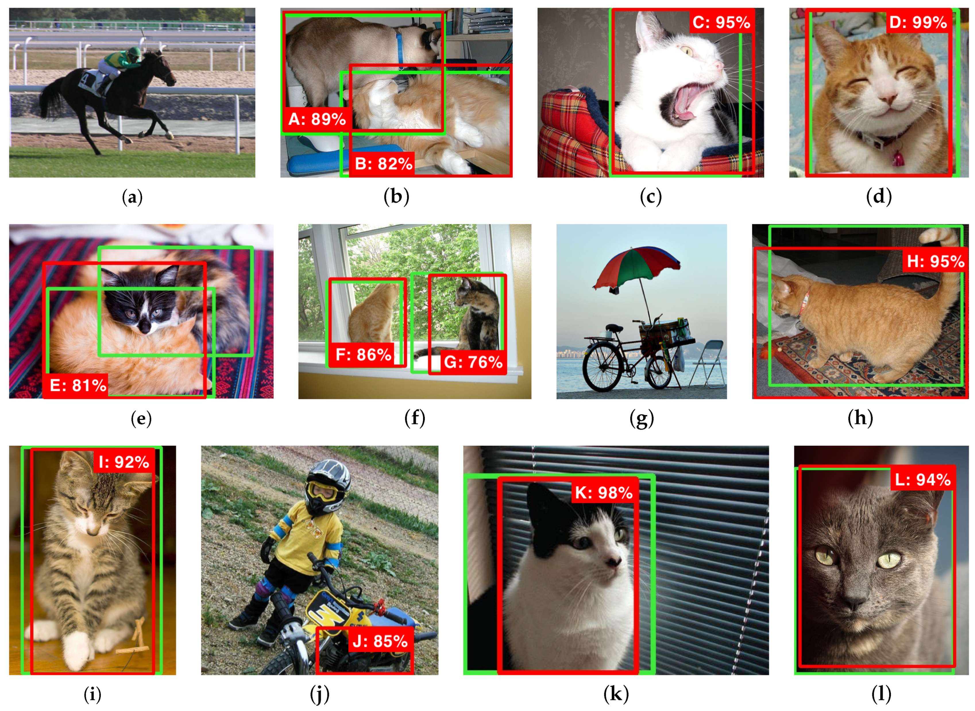
Considering the set of 12 images in Figure 3, each image, except (a), (g), and (j), has at least one target object of the class cat, whose ground-truth locations are delimited by the green rectangles. There is a total of 12 target objects limited by the green boxes. Images (b), (e), and (f) have each two ground-truth samples of the target class. An object detector predicted 12 objects represented by the red rectangles (labeled with letters ‘A’ to ‘L’) with their associated confidence levels being represented as percentages also shown close to the corresponding boxes. From the above, images (a), (g), and (j) are expected to have no detection, and images (b), (e), and (f) are expected to have two detections each.

All things considered, to evaluate the precision and recall of the 12 detections it is necessary to establish an IOU threshold t, which will classify each detection as TP or FP. In this example, let us first consider as TP the detections with $\mathrm{IOU}>50\%$, that is $t=0.5$.

As stated before, AP is a metric that integrates precision and recall in different confidence values. Thus, it is necessary to count the amount of TP and FP classifications given the different confidence levels.

Table 3. Precision and recall values for detections in Figure 3, that contain a total of 12 ground truths, considering an IOU threshold $t=0.5$.

Bounding Box	Confidence$\left(\mathit{\tau }\right)$	IOU	IOU > 0.5?	∑TP$\left(\mathit{\tau }\right)$	∑FP$\left(\mathit{\tau }\right)$	Pr$\left(\mathit{\tau }\right)$	Rc$\left(\mathit{\tau }\right)$
D	99%	0.91	Yes	1	0	1.0000	0.0833
K	98%	0.70	Yes	2	0	1.0000	0.1667
C	95%	0.86	Yes	3	0	1.0000	0.2500
H	95%	0.72	Yes	4	0	1.0000	0.3333
L	94%	0.91	Yes	5	0	1.0000	0.4167
I	92%	0.86	Yes	6	0	1.0000	0.5000
A	89%	0.92	Yes	7	0	1.0000	0.5833
F	86%	0.87	Yes	8	0	1.0000	0.6667
J	85%	-	No	8	1	0.8889	0.6667
B	82%	0.84	Yes	9	1	0.9000	0.7500
E	81%	0.74	Yes	10	1	0.9091	0.8333
G	76%	0.76	Yes	11	1	0.9167	0.9167

presents each detection from our example sorted by their confidence levels. In this table, columns ∑TP$\left(\tau \right)$ and ∑FP$\left(\tau \right)$ are the accumulated TPs and FPs, respectively, whose corresponding confidence levels are larger than or equal to the confidence $\tau$ specified in the second column of the table. Precision ($\mathit{Pr}\left(\tau \right)$) and recall ($\mathit{Rc}\left(\tau \right)$) values are calculated based on Equations (4) and (5), respectively. In this example a detection is considered as a TP only if its IOU is larger than 50%, and in this case the column ‘IOU > 0.5?’ is marked as ‘Yes’, otherwise it is marked as ‘No’ and is considered an FP. In this example, all detections overlap some ground-truth with $\mathrm{IOU}>0.5$, except detection ‘J’, which is not overlapping any ground-truth, so there is no IOU to be computed in this case.

Some detectors can output one detection overlapping multiple ground truths, as seen in the image from Figure 3b with detections ‘A’ and ‘B’. As detection ‘A’ has a higher confidence than ‘B’ ($89\%>82\%$), ‘A’ has the preference over ‘B’ to match the ground-truth, so ‘A’ is associated with the ground truth which gives the highest IOU. Figure 4c,d show the two possible associations that ‘A’ can have, ending up with the first one, which presents a higher IOU. Detection ‘B’ is left with the remaining ground truth in Figure 4f. Another similar situation where one detection could be associated with more than one ground truth is faced by detection ‘E’ in Figure 3e. The application of the same rule results in matching detection ‘E’ with the ground truth whose IOU is the highest, represented by the fairer cat, at the bottom of the image.

By choosing a more restrictive IOU threshold, different precision $\mathit{Pr}\left(\tau \right)$ and recall $\mathit{Rc}\left(\tau \right)$ values can be obtained.

Table 4. Precision and recall values for detections in Figure 3, that contain a total of 12 ground truths, considering an IOU threshold $t=0.75$.

Bounding Box	Confidence ($\mathit{\tau }$)	IOU	IOU > 0.75?	∑TP$\left(\mathit{\tau }\right)$	∑FP$\left(\mathit{\tau }\right)$	Pr$\left(\mathit{\tau }\right)$	Rc$\left(\mathit{\tau }\right)$
D	99%	0.91	Yes	1	0	1.0000	0.0833
K	98%	0.70	No	1	1	0.5000	0.0833
C	95%	0.86	Yes	2	1	0.6667	0.1667
H	95%	0.72	No	2	2	0.5000	0.1667
L	94%	0.91	Yes	3	2	0.6000	0.2500
I	92%	0.86	Yes	4	2	0.6667	0.3333
A	89%	0.92	Yes	5	2	0.7143	0.4167
F	86%	0.87	Yes	6	2	0.7500	0.5000
J	85%	-	No	6	3	0.6667	0.5000
B	82%	0.84	Yes	7	3	0.7000	0.5833
E	81%	0.74	No	7	4	0.6364	0.5833
G	76%	0.76	Yes	8	4	0.6667	0.6667

computes the precision and recall values with a more strict IOU threshold of $t=0.75$. By that, it is noticeable the occurrence of more FP detections and less TP detections, thus reducing both the precision $\mathit{Pr}\left(\tau \right)$ and recall $\mathit{Rc}\left(\tau \right)$ values.

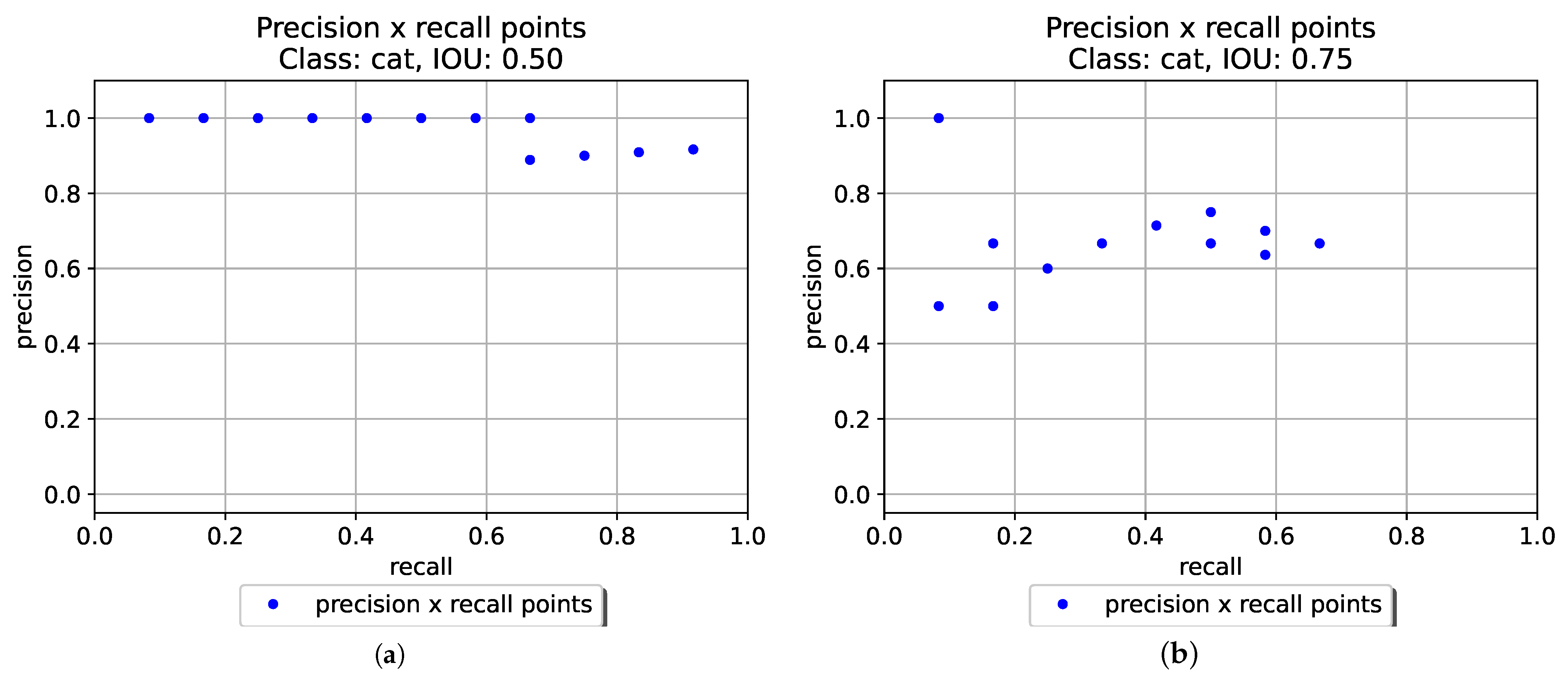
Graphical representations of the $\mathit{Pr}\left(\tau \right)$ × $\mathit{Rc}\left(\tau \right)$ values presented in Table 3 and Table 4 can be seen in Figure 5. By comparing both curves, one may note that for this example:

• With a less restrictive IOU threshold ($t=0.5$), higher recall values can be obtained with the highest precision. In other words, the detector can retrieve about $66.5\%$ of the total ground truths without any miss detection.
• Using $t=0.75$, the detector is more sensitive to different confidence values $\tau$. This is explained by the more accentuated monotonic behavior for this IOU threshold.
• Regardless the IOU threshold applied, this detector can never retrieve $100\%$ of the ground truths ($\mathit{Pr}\left(\tau \right)=1$) for any confidence value $\tau$. This is due to the fact that the algorithm failed to output any bounding box for one of the ground truths in Figure 3e.

Note that Figure 5 suggests that an IOU threshold of $t=0.5$ is less affected by different confidence levels. The graph for the lowest IOU threshold ($t=0.5$) shows that when confidence levels $\tau$ are high, the precision $\mathit{Pr}\left(\tau \right)$ does not vary, being equal to the maximum (1.0) for most of confidence values $\tau$. However, in order to detect more objects (increasing the recall $\mathit{Rc}\left(\tau \right)$), it is necessary to set a lower confidence threshold $\tau$, which reduces the precision at most by $12\%$. On the other hand, considering the highest IOU threshold ($t=0.75$), the detector can retrieve half of the target objects (recall = $0.5$) with a precision of $0.75$.

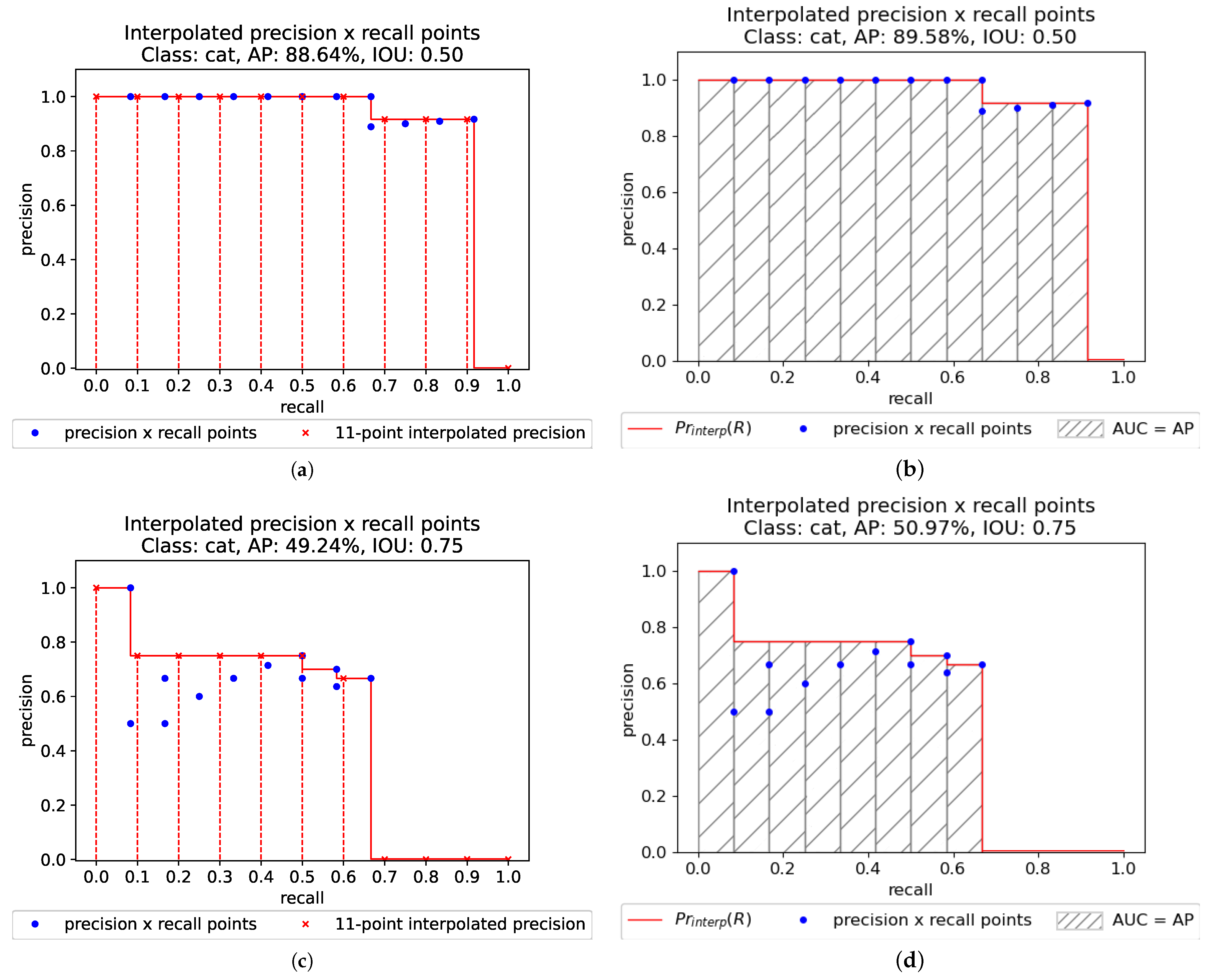
As previously explained, different methods can be applied to estimate the average precision, that is, the area under the precision × recall curve. To obtain AP using the N-point interpolation in Equation (11) with $N=11$ points, the area under the $\mathit{Pr}\times \mathit{Rc}$ curve is computed as the average of the interpolated precision ${\mathit{Pr}}_{\mathrm{interp}}\left(R\right)$ (Equation (9)) samples considering the sampling recall points R at $R_r\left(n\right)$ in the set $\{0,0.1,0.2,0.3,0.4,0.5,0.6,0.7,0.8,0.9,1.0\}$ (Equation (10)). On the other hand, to obtain AP using the all-point interpolation approach, the area under the $\mathit{Pr}\times \mathit{Rc}$ curve is computed by the Riemann integral in Equation (9), sampling the recall points R at $R_r\left(n\right)$ coincident with the $\mathit{Rc}\left(\tau \right)$ values given by the last column of Table 3 or of Table 4 (Equation (12)). The results can be seen in Figure 6. When an IOU threshold $t=0.5$ was applied, the 11-point interpolation method obtained $\mathrm{AP}=88.64\%$ while the all-point interpolation method resulted in a slightly higher AP, reaching $\mathrm{AP}=89.58\%$. Similarly, for an IOU threshold $t=0.75$, the 11-point interpolation method obtained $\mathrm{AP}=49.24\%$ and the all-point interpolation obtained $\mathrm{AP}=50.97\%$.

When a lower IOU threshold t was considered ($t=0.5$ as opposed to $t=0.75$), the AP was considerably increased in both interpolation approaches. This is caused by the increase in the TP detections, due to a lower IOU threshold.

If focus is shifted towards how well localized the detections are, irrespective of their confidence values, it is sensible to consult the AR metrics (Equations (14)–(18)). Computing twice the average excess IOU for the samples in this practical example as in Equation (15), yields $\mathrm{AR}=60\%$, while computing the average max recall across the standard COCO IOU thresholds, that is $t\in \{0.50,0.55,\dots ,0.95\}$, as in Equation (17), yields $\mathrm{AR}=66\%$. As the latter computation effectively does a coarser quantization of the IOU space, the two AR figures differ slightly. The next section enlists and briefly describes which variations of the metrics based on AP and AR are more frequently employed in the literature. In most cases they are the result of combinations of different IOU thresholds and interpolation methods.

6. Most Employed Metrics Based on AP and AR

As previously presented, there are different ways to evaluate the area under the precision × recall and recall × IOU curves. Nonetheless, besides such combinations of different IOU thresholds and interpolation points, that are other variations that result in different metric values. Some methods limit the evaluation by object scales and detections per image. This section overviews the distinctions behind all the metrics shown in Table 2.

6.1. AP with IOU Threshold $t=0.5$

This AP metric is widely used to evaluate detections in the PASCAL VOC dataset [67]. Its official implementation is in MATLAB and it is available in the PASCAL VOC toolkit. It measures the AP of each class individually by computing the area under the precision × recall curve interpolating all points as presented in Equation (9). In order to classify detections as TP or FP the IOU threshold is set to $t=0.5$.

6.2. mAP with IOU Threshold $t=0.5$

This metric is also used by the PASCAL VOC dataset and is also available in their MATLAB toolkit. It is calculated as the AP with IOU $t=0.5$, but the result obtained by each class is averaged as given in Equation (13).

6.3. AP@.5 and AP@.75

These two metrics evaluate the precision × recall curve differently than the PASCAL VOC metrics. In this method, the interpolation is performed in $N=101$ recall points, as given in Equation (11). Then, the computed results for each class are summed up and divided by the number of classes, as in Equation (13).

The only difference between AP@.5 and AP@.75 regards the applied IOU thresholds. AP@.5 uses $t=0.5$ whereas AP@.75 applies $t=0.75$. These metrics are commonly used to report detections performed in the COCO dataset and are officially available in their official evaluation tool.

6.4. AP@[.5:.05:.95]

This metric expands the AP@.5 and AP@.75 metrics by computing the AP@ with 10 different IOU thresholds ($t=[0.5,0.55,...,0.95]$) and taking the average among all computed results.

6.5. AP_S, AP_M, and AP_L

These three metrics, also referred to as AP Across Scales, apply the AP@[.5,.05:.95] from Section 6.1 taking into consideration the area of the ground-truth object:

• AP_S only evaluates small ground-truth objects (area < ${32}^2$ pixels);
• AP_M only evaluates medium-sized ground-truth objects (${32}^2$ < area < ${96}^2$ pixels);
• AP_L only evaluates large ground-truth objects (area > ${96}^2$).

When evaluating objects of a given size, objects of the other sizes (both ground-truth and predicted) are not considered in the evaluation. This metric is also part of the COCO evaluation dataset.

6.6. AR₁, AR₁₀, and AR₁₀₀

These AR variations apply Equation (14) limiting the number of detections per image, that is, they calculate the AR given a fixed amount of detections per image, averaged over all classes and IOUs. The IOUs used to measure the recall values are the same as in AP@[.5,.05:.95].

AR₁ considers up to one detection per image, while AR₁₀ and AR₁₀₀ consider at most 10 and 100 objects per image, respectively.

6.7. AR_S, AR_M and AR_L

Similarly to the AR variations with limited number of detections per image, these metrics evaluate detections considering the same areas as the AP across scales. As the metrics based on AR are implemented in the COCO official evaluation tool, they are regularly reported with the COCO dataset.

6.8. F1-Score

The F1-score is defined as the harmonic mean of the precision ($\mathit{Pr}$) and recall ($\mathit{Rc}$) of a given detector, that is:

$${\mathrm{F}}_1=2\frac{\mathit{Pr}.\mathit{Rc}}{\mathit{Pr}+\mathit{Rc}}=\frac{\mathrm{TP}}{\mathrm{TP}+\frac{\mathrm{FN}+\mathrm{FP}}{2}}.$$

(19)

The F1-score is limited to the interval [0, 1], being 0 if precision or recall (or both) are 0, and 1 when both precision and recall are 1.

As the F1-score does not take into account different confidence values, it is only used to compare object detectors in a fixed confidence threshold level $\tau$.

6.9. Other Metrics

Other less popular metrics have also been proposed to evaluate object detections. They are mainly designed to be applied with particular datasets. The Open Images Object Detection Metric, for example, is similar to mAP (IOU=.50), being specifically designed to consider special ground-truth annotations of the Open Images dataset [68]. This dataset groups into a single annotation five or more objects of the same class that somehow are occluding each other, such as a group of flowers or a group of people. This metric simply ignores a detection if it overlaps a ground-truth box tagged as group of, whose area of intersection between the detection and ground-truth boxes divided by the area of the detection is greater than 0.5. This way, it does not penalize detections matching a group of very close ground-truth objects.

The localization recall-precision (LRP) error, a new metric suggested in [91], intends to consider the accuracy of the detected bounding box localization and equitably evaluate situations where the AP is unable to distinguish very different precision × recall curves.

6.10. Comparisons among Metrics

In practice, the COCO’s AP@[.5:.05:.95] and PASCAL mAP metrics are the most popular ones used as benchmarks. However, as COCO’s AP@[.5:.05:.95] is affected by different IOUs, it is not possible to evaluate the effectiveness of the detector with a more or less restrictive IOU with this metric. For a more strict evaluation with respect to the likeness of the ground truth and detection bounding boxes, the AP@.75 metric should be applied. In datasets where the objects appear to have relatively different sizes, AP metrics concerning their areas should be employed. By that, the assertiveness of objects with similar relative sizes can be compared. As shown in this work, the interpolation methods applied by the AP metrics try to remove the non-monotonic behavior of the $\mathit{Pr}\left(\tau \right)\times \mathit{Rc}\left(\tau \right)$ curve before calculating its AUC. In an N-point interpolation, a greater N leads to a better AUC approximation. Therefore, the 101-point interpolation approach used by COCO’s AP metrics provides a better AUC approximation than the 11-point interpolation approach. On the other hand, PASCAL VOC uses the all-point interpolation, which is an even better approximation of the AUC. In cases where the detector is expected to detect at least a certain amount of objects in a given image (e.g., detecting one bird in a flock of birds should be sufficient), AR metrics regarding detections or sizes are more appropriate.

7. Evaluating Object Detection in Videos

Many works in the literature use the mAP as a metric to evaluate the performance of object detection models in video sequences [92,93,94,95,96,97,98]. In this case, the frames are evaluated independently, ignoring the spatio-temporal characteristics of the objects presented in the scene. The authors of [92] categorized the ground-truth objects according to their motion speed. This is done by measuring the average IOU score of the current frame and the nearby $\pm 10$ frames. In this context, in addition to mAP, they also reported the mAP over the slow, medium, and fast groups, denoted as mAP(slow), mAP(medium), and mAP(fast), respectively.

In some applications, the latency in the identification of the objects of interest plays a crucial role in how well the overall system will perform. Detection delay, defined as the number of frames between the first occurrence of an object in the scene and its first detection, then becomes an important measurement for time-critical systems. The authors in [99] claim that AP is not sufficient to quantify the temporal behavior of detectors, and propose a complementary metric, the average delay (AD), averaging the mean detection delay over multiple false positive ratio thresholds, and over different object sizes, yielding a metric that fits well for systems that rely on timely detections. While the cost of detection latency is significant for a somewhat niche set of tasks, the inclusion of time information for video detection metrics can be useful to assess system behaviors that would otherwise be elusive when only the standard, frame level AP metric is used.

7.1. Spatio-Temporal Tube Average Precision

As discussed above, the aforementioned metrics are all used on an image or frame level. However, when dealing with videos, one may be interested in evaluating the model performance at the whole video level. In this work, we propose an extension of the AP metric to evaluate video object detection models that we refer to as spatio-temporal tube AP (STT-AP). As in AP, a threshold over the IOU is also used to determine whether the detections are correct or not. However, instead of using two types of overlaps (spatial and temporal), we extend the standard IOU definition to consider the spatio-temporal tubes generated by the detection and of the ground truth. This metric, that integrates spatial and temporal localizations, is concise, yet expressive.

Instead of considering each detection of the same object independently along the frames, the spatial bounding boxes of the same object are concatenated along the temporal dimension, forming a spatio-temporal tube, which is the video analogous to an image bounding box. A spatio-temporal tube $T_o$ of an object o is the spatio-temporal region defined as the concatenation of the bounding boxes of this object from each frame of a video, that is:

$$T_o=\left[\begin{array}{c}{B}_{o,q}{B}_{o,q+1}\cdots B_{o,q+Q-1}\end{array}\right],$$

(20)

where $B_{o,k}$ is the bounding box of the object o in frame k of the video that is constituted of Q frames indexed by $k=q,q+1,\dots ,q+Q-1$.

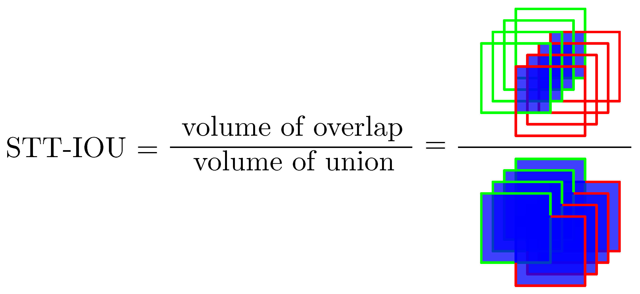
Using spatio-temporal tubes, the concept of IOU used in object detection in images (see Section 4) can be naturally extended to videos. Considering a ground-truth spatio-temporal tube $T_{\mathit{gt}}$ and a predicted spatio-temporal tube $T_p$, the spatio-temporal tube IOU (STT-IOU) measures the ratio of the overlapping to the union of the “discrete volume” between $T_{\mathit{gt}}$ and $T_p$, such that:

$$\mathrm{STT}\text{-}\mathrm{IOU}=\frac{\mathrm{volume}(T_p\cap T_{\mathit{gt}})}{\mathrm{volume}(T_p\cup T_{\mathit{gt}})}=\frac{{\displaystyle \sum _k\mathrm{area}\mathrm{of}\mathrm{overlap}\mathrm{in}\mathrm{frame}k}}{{\displaystyle \sum _k\mathrm{area}\mathrm{of}\mathrm{union}\mathrm{in}\mathrm{frame}k}},$$

(21)

as illustrated in Figure 7.

In this way, an object is considered a TP if the STT-IOU is equal or greater than a chosen threshold. As in the conventional AP, this metric may be as rigorous as desired. The closer to 1 it is, the more well-located the predicted tube must be to be considered a TP.

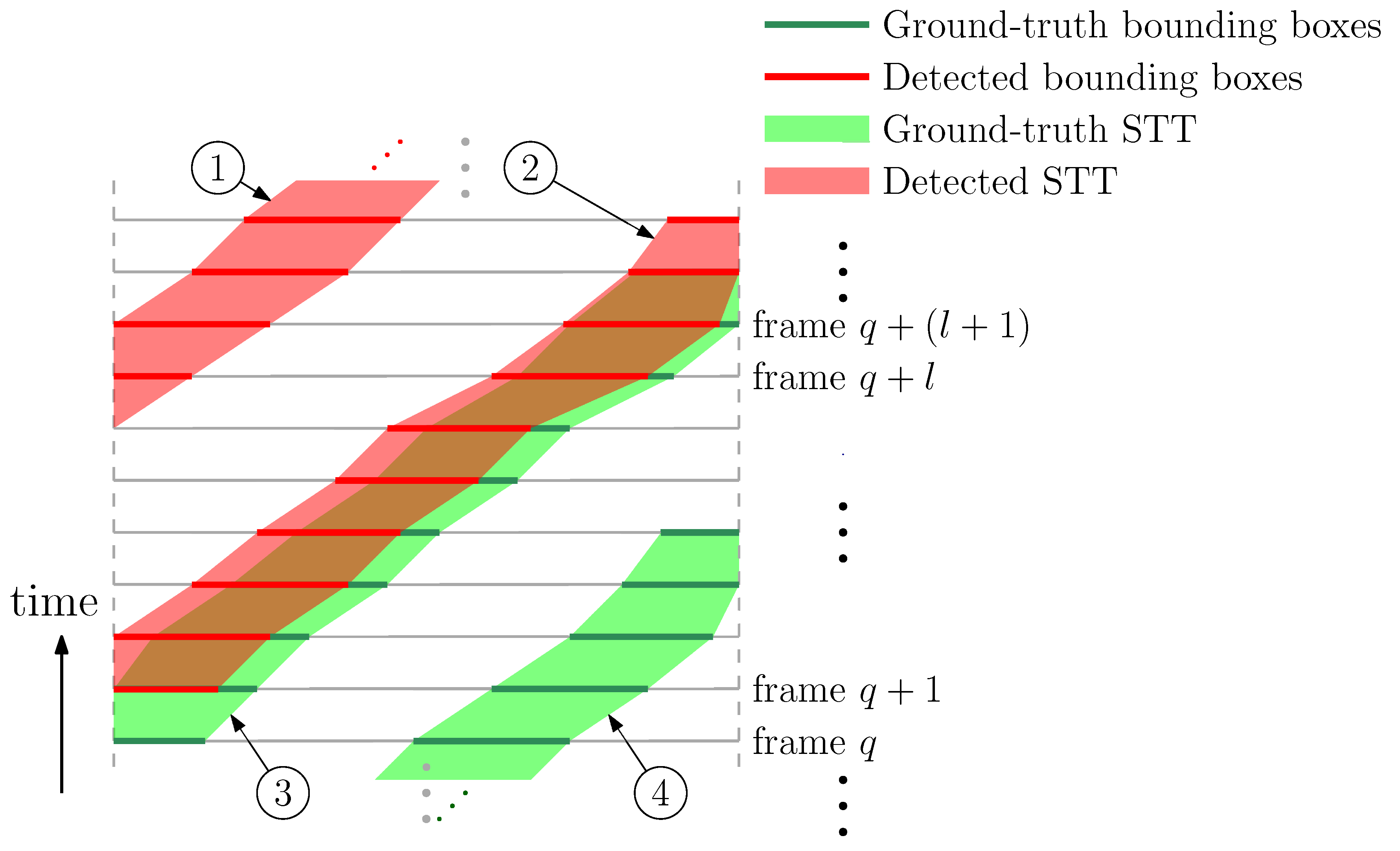
Figure 8 illustrates four different STTs. The STTs in red are detected STTs and the STTs in green are ground-truth STTs. The STT in (1) constitutes an FP case, and the STT in (2) may be a TP case (depending on the STT-IOU), as it intersects the corresponding ground-truths STT (3). Since there is no detection corresponding to the ground-truth STT (4), it is an FN.

Based on these definitions, the proposed STT-AP metric follows the AP: For each class, each ground-truth tube is associated with the predicted tube of the same class that presents the highest STT-IOU scores (since it is higher than the threshold). The ground-truth tubes not associated with a predicted tube are FNs and the predicted tubes not associated with a ground-truth tube are FPs. Then, the spatio-temporal tube predictions are ranked according to the predicted confidence level (from the highest to the lowest), irrespective of correctness. Since the STT-AP evaluates the detection of an object in the video as a whole, the confidence level assumed for a spatio-temporal tube is the average confidence of the bounding boxes corresponding to each of its constituent frames. After that, the all-point interpolation (Section 4.2.2) is performed allowing one to compute the proposed STT-AP. This procedure may be repeated and averaged for all classes in the database, yielding the so-called mean STT-AP (mSTT-AP). From Equation (21) one can readily see that the computational cost per frame of the SST-AP is similar to the one of the frame-by-frame mAP.

8. An Open-Source Toolbox

This paper focuses on explaining and comparing the different metrics and formats currently used in object detection, detailing the specifications and pointing out the particularities of each metric variation. The existing tools provided by popular competitions [24,81,82,83,84,85] are not adequate to evaluate metrics using annotations in formats that are different from their native ones. Thus, to complement the analysis of the metrics presented here, the authors have developed and released an open-source toolkit as a reliable source of object detection metrics for the academic community and researchers.

With more than 3100 stars and 740 forks, our previously available tool for object detection assessment [100] has received positive feedback from the community and researchers. It has also been used as the official tool in competition [86], adopted in 3rd-party libraries such as [101], and parts of our code have been used by many other works such as in YoloV5 [9]. Besides the significant acceptance by the community, we have received many requests to expand the tool in order to support new metrics and bounding box formats. Such demands motivated us to offer more evaluation metrics, to accept more bounding box formats, and to present a novel metric for object detection in videos.

This tool implements the same metrics used by the most popular competitions and object-detection benchmark researches. This implementation does not require modifications of the detection model to match complicated input formats, avoiding conversions to XML, JSON, CSV, or other file types. It supports more than eight different kinds of annotation formats, including the ones presented in Table 1. To ensure the accuracy of the results, the implementation strictly followed the metric definitions and the output results were carefully validated against the ones of the official implementations.

Developed in Phython and supporting 14 object detection metrics for images, this work also incorporates the novel spatio-temporal metric described in Section 7.1 to evaluate detected object in videos aggregating some of the concepts applied to evaluate detections in images. From a practical point of view, the tool can also be adapted and expanded to support new metrics and formats. The expanded project distributed with this paper can be accessed at https://github.com/rafaelpadilla/review_object_detection_metrics [102].

9. Metrics Evaluation in a Practical Example

In this section, we use different object detection metrics to evaluate YOLOv5 model [9]. The chosen model was trained with the COCO dataset and was applied in the training/validation PASCAL VOC 2012 dataset [67]. Intentionally different datasets were used to train and evaluate the model to evidence the potential of our tool to deal with different ground-truth and detected bounding-box formats. For this experiment, the annotations of the ground-truth boxes are in PASCAL VOC format containing 20 classes of objects, while the model was trained with COCO dataset and was able to detect objects in 80 classes, predicting detections in text files in the YOLO format.

By using our tool, one can quickly obtain 14 different metrics without the necessity to convert files to specific formats. As some classes of the ground-truth dataset are tagged differently by the detector (e.g., PASCAL VOC class tvmonitor is referred to as tv in COCO dataset), the only required work is to provide a text file listing the names of the classes in the ground-truth format. This way the evaluation tool can recognize that the detected object airplane should be evaluated as aeroplane.

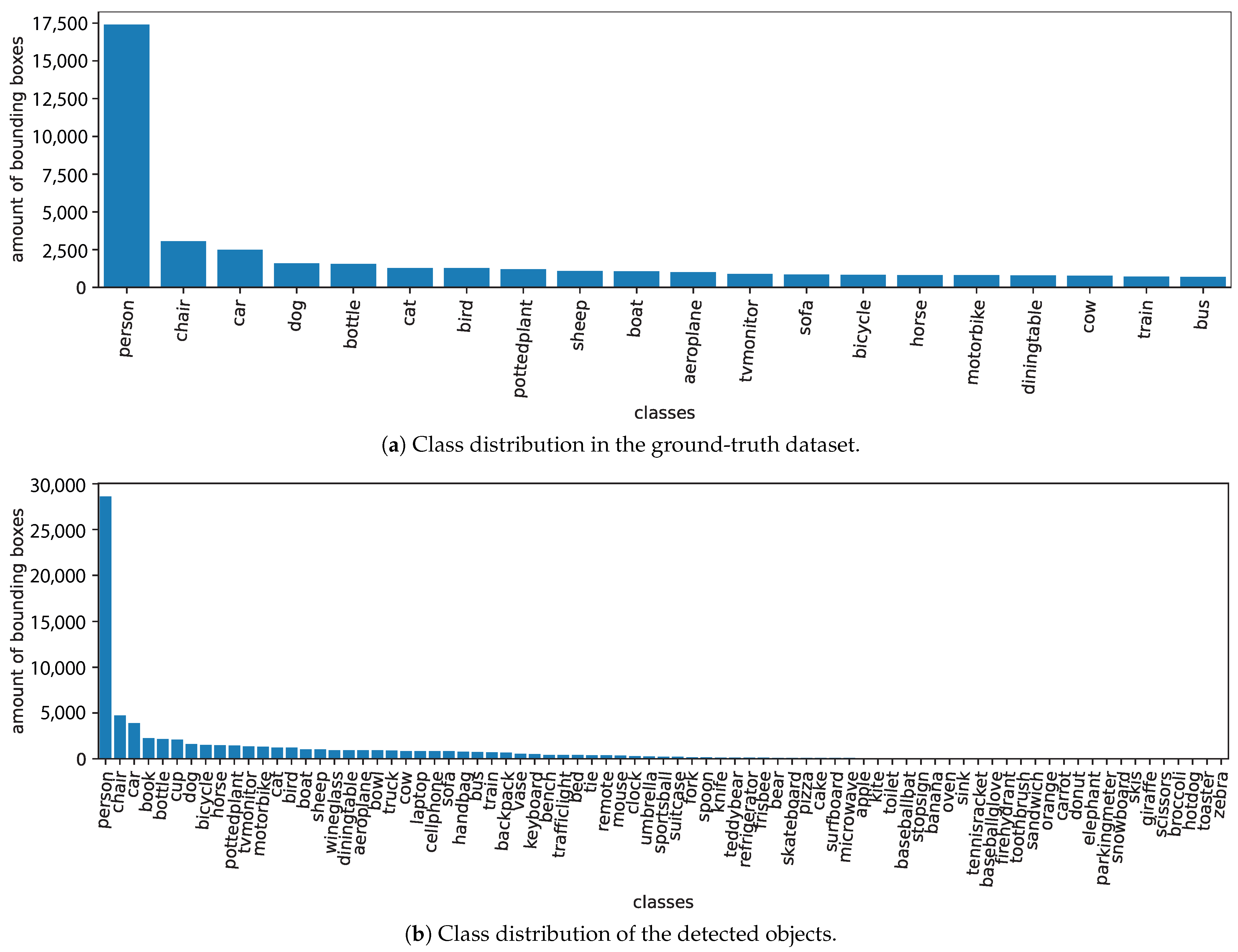
A total of $17,125$ of images from the train/val PASCAL VOC 2012 dataset containing $40,138$ objects of 20 classes were evaluated by the YOLOV5 model to detect objects in 80 different classes. A total of $74,752$ detections were detected by the model. Figure 9 compares the distribution of ground-truth and detected objects per class. Due to the difference of classes in the training and testing datasets, many predicted classes are not in the ground-truth set, so detections of the extra classes are ignored by the metrics.

The AP results for each class are presented in

Table 5. AP results obtained with different interpolation methods and IOU thresholds.

Class	IOU Threshold = 0.5			IOU Threshold = 0.75
	101-Point	11-Point	All-Point	101-Point	11-Point	All-Point
aeroplane	0.76	0.79	0.77	0.57	0.58	0.58
bicycle	0.41	0.43	0.41	0.31	0.33	0.31
bird	0.66	0.67	0.66	0.49	0.48	0.50
boat	0.47	0.46	0.47	0.28	0.29	0.29
bottle	0.45	0.47	0.45	0.32	0.34	0.33
bus	0.79	0.78	0.80	0.74	0.69	0.74
car	0.52	0.53	0.53	0.39	0.39	0.39
cat	0.73	0.74	0.73	0.54	0.53	0.54
chair	0.41	0.40	0.41	0.30	0.32	0.30
cow	0.74	0.69	0.74	0.59	0.58	0.60
diningtable	0.44	0.46	0.44	0.28	0.31	0.28
dog	0.66	0.64	0.65	0.53	0.53	0.53
horse	0.42	0.43	0.43	0.35	0.36	0.35
motorbike	0.51	0.53	0.51	0.38	0.39	0.38
person	0.67	0.65	0.68	0.53	0.54	0.53
pottedplant	0.37	0.39	0.37	0.22	0.25	0.22
sheep	0.68	0.68	0.68	0.56	0.58	0.57
sofa	0.44	0.45	0.44	0.37	0.38	0.37
train	0.75	0.77	0.76	0.65	0.66	0.65
tvmonitor	0.54	0.55	0.54	0.43	0.45	0.43
average	0.57	0.58	0.57	0.44	0.45	0.44

. The highest AP values over all classes were obtained when the AUC was measured with the 11-point interpolation method and an IOU threshold of $t=0.5$, resulting in $mAP=0.58$. As expected for all cases, a more rigorous IOU threshold ($t=0.75$) resulted in a smaller AP. Comparing the individual AP results among all classes, the most difficult object for all interpolation methods was the potted plant, having an AP not higher than $0.37$ for an IOU threshold of $t=0.5$ and an AP not higher than $0.22$ with an IOU threshold of $t=0.75$.

The results obtained by the variations which apply AP and AR with different sizes and quantity of objects per image are summarized in

Table 6. Values of AP and average recall (AR) variations for different object sizes and number of detections per image.

Metric	Result
APS	0.13
APM	0.33
APL	0.46
AR1	0.39
AR10	0.53
AR100	0.53
ARS	0.23
ARM	0.47
ARL	0.58

.

Even if the same interpolation technique is applied, the results may vary depending on the IOU threshold. Similarly, different interpolations with the same IOU threshold may also lead to distinct results.

The metrics considering objects in different scales are useful to compare the assertiveness of detections in datasets containing objects of different scales. In the COCO dataset, for instance, roughly $42\%$ of the objects are considered small (area < ${32}^2$ pixels), $34\%$ are considered medium (${32}^2$ < area < ${96}^2$ pixels), and $24\%$ are considered large (area > ${96}^2$ pixels). This explains the vast amount of works using this dataset to report their results.

10. Conclusions

This work analyzed the formats of bounding boxes used to represent the objects in popular datasets, demonstrated the most common benchmark object detection metrics, and suggested a new metric for videos, the spatio-temporal tube average precision (STT-AP), based on the concepts used to evaluate object detection in images. The similarities and inconsistencies of each metric were examined, and our results revealed their dissimilarities by evaluating the predictions of a pre-trained object detector in a largely used dataset. A toolkit implementing all described metrics in a way compatible to most data-annotation formats in use was presented and validated. Such results may facilitate direct and unified comparisons among most algorithms being proposed in the field of object detection. For future work, we intend to perform a regular survey update through its companion website, incorporating newly proposed metrics and annotation formats, and extend it to the problem of object tracking.