Development and Simulation of Motion Control System for Small Satellites Formation

Abstract

In the paper, the problem of forming and maintaining the small satellites formation in the near-earth projected circular orbits is considered. The satellite formation reconfiguration and formation-keeping control laws are proposed by employing the passivity-based output feedback control. For the complete nonlinear and time-dependent dynamics of the relative motion of a pair of satellites in elliptical orbits, new combined control algorithms, including a consensus protocol, are proposed and analyzed. A comparison of the control modes using the passivity-based output feedback control and the proportional-differential controller with and without the consensus algorithm is given. On the basis of the passification method, the algorithm is obtained ensuring the stable motion of the slave satellite relative to the orbit of the master satellite. To improve the accuracy of the satellites’ positioning, a consensus protocol based on measurements of the relative positions of the satellites is proposed and studied. Computer simulations of the proposed algorithms for options to construct formations are provided for two projected circular orbits of 8 satellites, demonstrating the efficiency of the proposed control schemes. It is shown that the resulting passivity-based output feedback control provides better accuracy than the PD controller. It is also shown that the use of the consensus protocol further increases the positioning accuracy of the satellite constellation.

1. Introduction

Space research has led to the emergence of the idea of spacecrafts’ motion in a group. Group motion makes it possible to perform a wider range of tasks. This approach has reduced the costs of production and operation, and increased the reliability of the entire system. There are several satellite constellation formation methods for creating time-invariant and time-varying configurations. In the literature, various options to create satellite constellations are proposed, cf. [1,2,3]. The constant tuning method [4] implies periodic adjustment of active satellites relative to the spatial position. The variable formation method [5] forms a swarm, which periodically changes its configuration as satellites move in non-coplanar orbits. It is possible to form the configuration of satellites by means of their tether connection; such formations are possible in low orbits [6]. A grouping can be formed using several methods; this method of formation is called combined [2]. Among the groupings with a constant structure, a class stands out that uses projected circular orbits (PCO) [7] to form the structure. When using this construction method, a group is considered, which consists of the head and surrounding slave satellites [8]. The orbit of the master satellite is considered to be the reference orbit, and the remaining orbits are called projection circular orbits, which are circular when projected onto the local horizontal plane [9,10]. The first successful missions were based on the results for a group of two satellites [11]. Based on these results, a mission was implemented to study the formation of satellites in near-earth orbit. Two satellites, CanX-4 and CanX-5 [12], were launched. The satellites maintained a maximum controllable range of about 50 m. The satellites under study are classified as small. For these satellites, various options were proposed to solve the problem of building a permanent group structure. However, there are still problems associated with their control. One of them is the need to keep the satellites in a prescribed order. A number of studies were carried out to address this problem. As an example, in [13,14,15], various methods of adaptive control of the spacecraft formation were considered. In [16], the variable structure model reference adaptive control technique for spacecraft formation flying was proposed. Zou and Kumar [17] presented the fast terminal sliding manifold, using a control term based on the hyperbolic tangent function to suppress bounded external disturbances. The control system for such plants is designed to solve many problems. One of these tasks is to keep a constant satellite configuration. For this, the method of stabilizing only the unstable subsystem can be applied. In [18,19,20], a partial stabilization method with an algorithm to compensate for fluctuations was applied. These studies consider the stabilization of a linearly varying component caused by a zero root of multiplicity two. Additionally, a method to maintain satellite configuration employs the PCO.

In [21,22], the control of a formation of two satellites in a near-earth circular orbit is discussed. It is proposed to use adaptive neurocontrol. One of the vehicles is considered to be controllable, while the second is uncontrolled and moves in PCO orbit relative to the first satellite. To solve the adaptation problem, a non-gradient optimization method is used. Adaptation takes $2.5$ to 5 days. This approach is time consuming to control a large group of satellites. In [5], a feedback control law was developed to regulate the relative motion of satellites in a swarm in a low circular near-earth orbit, taking into account the speed of data transmission over communication channels. The control law is based on classical modal control. In [23], algorithms were developed for decentralized stabilization of the position of two satellites moving in a near circular orbit using a modal approach, passification method, sliding mode control, linear and speed-optimal partial stabilization. In the study of a new control algorithm based on the passification method, convergence was obtained at a lower initial speed than the modal control algorithm. Ref. [24] discussed maintaining a working orbit and a given configuration. For the orbit of the lead satellite, rigid (absolute) support is used. For the slave satellite, rigid and flexible (relative) support is applied. The dependence of the costs of the total characteristic velocity to maintain the master and slave vehicles on the accuracy of maintaining the working orbit was investigated, which showed the particular importance of the correct choice of the maximum accuracy of maintaining. In [25], the problem of calculating the parameters of the maneuvers of the satellite system configuration was considered. For convenience, the orbits of a group of six satellites (STARSIS) are reduced to projection circular orbits. Ref. [26] complemented the task of calculating the parameters of satellite maneuvers by examining high-elliptic orbits for four satellites. The satellite array model is brought into the main orbital plane to simplify calculations. In [27], to solve the control problem, the influence of the given initial values of the projection circular orbit for different approaches to control of a group of satellites was investigated. The design takes into account the minimization of error and fuel consumption.

When performing tasks with a large number of satellites, it is more efficient to use multi-agent and decentralized control [28]. To this aim, in [4], using local relative dimensions was suggested. Another approach was used in the article [29]. It proposed a combined consensus method with a robust $H_{\infty }$ control. Using this approach, it is possible to provide an arbitrary scalability of the system. Comparisons were made between various controllers [30]. In the course of the study, data were obtained, on the basis of which it was shown that the nonlinear controller based on the Riccati equations (state-dependent Riccati equation—SDRE) has better accuracy.

The paper is devoted to the problem of forming and maintaining the small satellites formation in the near-earth PCO orbits. On the basis of the passification method, an algorithm is obtained that ensures the stable motion of the slave satellite relative to the orbit of the master satellite. To improve the accuracy of satellites positioning, a consensus protocol based on measurements of the relative positions of satellites is proposed and studied.

In this paper, for the complete nonlinear and time-dependent dynamics of the relative motion of a pair of satellites in elliptical orbits, new combined control algorithms, including a consensus protocol, are proposed and analyzed. A comparison of the control modes using the PD controller with and without the consensus algorithm is given. The dynamic structure of the proposed control algorithm is quite simple and avoids the use of a large number of blocks. Its implementation is simple, and the computational cost is low. The new result of the paper is also a rigorous mathematical proof of the use of control laws based on the passification method for the satellite system under consideration.

The rest of the paper is organized as follows. Section 2 is devoted to modeling the satellite formation. The problem statement is given in Section 3. Section 4 deals with application of the passivity concept to the control law design. The notion of projection circular orbit is described in Section 5. Section 6 presents designing the control law for PCO constellation. The simulation results are given in Section 8. Concluding remarks in Section 9 finalize the paper.

2. Satellite Formation Modeling

In satellite formation flying, the relationship of the positions between satellites is very important. Hence, the rotating reference coordinate is used: a chief satellite is centrally located and circles the Earth. Note that it is assumed that the main satellite is located at the origin of the coordinate system because it provides a reference point for the formation. The local-vertical local-horizontal (LVLH) coordinate system [1] is used to describe the relative motion in the formation.

The coordinate systems are illustrated in Figure 1. In this figure, ${\overrightarrow{r}}_{\mathrm{c}}$ is the position vector of the master satellite, $\overrightarrow{r}$ is the position vector of the slave satellite, and $\overrightarrow{\rho }$ is the relative position vector between the master and slave satellites. A general non-linear equation of relative motion is expressed as in [1]:

$$\begin{array}{c}\left[\begin{array}{c}\ddot{x}-2\dot{\theta }\dot{y}-\ddot{\theta }y-{\dot{\theta }}^{2}x+{\displaystyle \frac{\mu }{\gamma }}x+{\displaystyle \frac{\mu }{\gamma }}{r}_{\mathrm{c}}-{\displaystyle \frac{\mu }{r_{\mathrm{c}}^2}}\\ \ddot{y}+2\dot{\theta }\dot{x}+\ddot{\theta }x-{\dot{\theta }}^{2}y+{\displaystyle \frac{\mu }{\gamma }}y\\ \ddot{z}+\frac{\mu }{\gamma }z\end{array}\right]=\left[\begin{array}{c}{a}_{\mathrm{x}}\\ a_{\mathrm{y}}\\ a_{\mathrm{z}}\end{array}\right]\end{array}$$

(1)

$$\begin{array}{c}{\ddot{r}}_{\mathrm{c}}=r_{\mathrm{c}}{\dot{\theta }}^2-\frac{\mu }{r_{\mathrm{c}}^2},\ddot{\theta }=-\frac{2{\dot{r}}_{\mathrm{c}}\dot{\theta }}{r_{\mathrm{c}}}\end{array}$$

(2)

where x, y and z are state variables to describe the relative position vector, $\overrightarrow{\rho }$, in the $x,y$ and z axes, respectively, and $a_{\mathrm{x}}$, $a_{\mathrm{y}}$ and $a_{\mathrm{z}}$ are the orbital perturbation terms, such as the aspherical geopotential perturbation, thrust, air drag, and solar radiation pressure. $a_j=(f_j+d_j)/m_{\mathrm{f}}$ for all $j\in \{x,y,z\}$ with $m_{\mathrm{f}}$ denoting the mass of the deputy spacecraft and $f_j$ denoting the control input applied by the deputy spacecraft, $d_j$ is for the perturbation term, $\theta$ is latitude angle of the chief, $r_{\mathrm{c}}$ is the radius of the chief orbit and $\mu$ is a gravitational parameter. Finally, $\gamma$ is defined as

$$\begin{array}{c}\hfill \gamma \equiv {\left|{\overrightarrow{r}}_{\mathrm{c}}+\overrightarrow{\rho }\right|}^3={\left({\left(r_{\mathrm{c}}+x\right)}^2+y^2+z^2\right)}^{3/2}.\end{array}$$

(3)

For controller design, it is desirable to rewrite system (1) in the following state-space form

$$\begin{array}{c}\hfill \dot{\mathbf{x}}=\mathbf{A}(\mathbf{x},t)\mathbf{x}+\mathbf{B}\mathbf{u},\end{array}$$

(4)

where the state variables are the relative positions and relative velocities of the deputy satellite with regard to the chief satellite

$$\begin{array}{c}\hfill \mathbf{x}={\left[\begin{array}{cccccc}x& y& z& \dot{x}& \dot{y}& \dot{z}\end{array}\right]}^{\mathrm{T}},\mathbf{u}={\left[\begin{array}{ccc}{f}_x\hfill & f_y\hfill & f_z\hfill \end{array}\right]}^{\mathrm{T}}\end{array}$$

It is assumed in this paper that all the system states are measured. Therefore, the full state feedback control can be implemented. Let us rewrite the term of $\left({\displaystyle \frac{\mu }{\gamma }}{r}_{\mathrm{c}}-{\displaystyle \frac{\mu }{r_{\mathrm{c}}^2}}\right)$ in (1) to preserve the non-linearity as much as possible and to avoid a singularity [30]. Using (3), this term can be expressed in the following form:

$$\begin{array}{c}\hfill \frac{\mu }{\gamma }{r}_{\mathrm{c}}-\frac{\mu }{{r_{\mathrm{c}}}^2}=\mu \left(\frac{r_{\mathrm{c}}}{{\left(1+\frac{2}{r_{\mathrm{c}}}x+\frac{x^2+y^2+z^2}{{r_{\mathrm{c}}}^2}\right)}^{3/2}}\frac{1}{{r_{\mathrm{c}}}^3}-\frac{1}{{r_{\mathrm{c}}}^2}\right)\end{array}$$

(5)

$$\begin{array}{c}\hfill =\frac{\mu }{{r_{\mathrm{c}}}^2}\left({\left(1-\left(-\frac{2}{r_{\mathrm{c}}}x-\frac{x^2+y^2+z^2}{r_{\mathrm{c}}^2}\right)\right)}^{-\frac{3}{2}}-1\right)\end{array}$$

(6)

Let us define

$$\xi \equiv -\frac{2}{r_{\mathrm{c}}}x-\frac{x^2+y^2+z^2}{{r_{\mathrm{c}}}^2}=\left(-\frac{2}{r_{\mathrm{c}}}-\frac{x}{{r_{\mathrm{c}}}^2}\right)x+\left(-\frac{y}{{r_{\mathrm{c}}}^2}\right)y+\left(-\frac{z}{{r_{\mathrm{c}}}^2}\right)z$$

(7)

Then, by negative binomial series and (5), (7) becomes:

$$\begin{array}{c}\hfill \begin{array}{c}\hfill \frac{\mu }{\gamma }{r}_{\mathrm{c}}-\frac{\mu }{{r_{\mathrm{c}}}^2}=\frac{\mu }{{r_{\mathrm{c}}}^2}\left({(1-\xi )}^{-\frac{3}{2}}-1\right)=\frac{\mu }{{r_{\mathrm{c}}}^2}\left(1+\frac{3}{2}\Psi \xi -1\right)=\frac{3}{2}\frac{\mu }{{r_{\mathrm{c}}}^2}\Psi \xi \end{array}\end{array}$$

(8)

where $\Psi$ is defined as a series $\Psi \equiv 1+{\psi }_1+{\psi }_2+\cdots$, where:

$$\begin{array}{c}\hfill \begin{array}{c}\hfill {\psi }_1\equiv \frac{\left(\frac{3}{2}+1\right)}{2}\xi ,{\psi }_2\equiv \frac{\left(\frac{3}{2}+2\right)}{3}{\psi }_1\xi ,{\psi }_3\equiv \frac{\left(\frac{3}{2}+3\right)}{4}{\psi }_2\xi ,\dots \end{array}\end{array}$$

Consequently, (1) becomes:

$$\begin{array}{cc}\hfill & \left[\begin{array}{c}{\dot{x}}_1\\ {\dot{x}}_2\\ {\dot{x}}_3\\ {\dot{x}}_4\\ {\dot{x}}_5\\ {\dot{x}}_6\end{array}\right]=\left[\begin{array}{cccccc}0& 0& 0& 1& 0& 0\\ 0& 0& 0& 0& 1& 0\\ 0& 0& 0& 0& 0& 1\\ {\dot{\theta }}^2-\frac{\mu }{\gamma }+\frac{3}{2}\frac{\mu }{r_{\mathrm{c}}^3}\left(2+\frac{x}{r_{\mathrm{c}}}\right)\Psi & 0& \ddot{\theta }+\frac{3}{2}\frac{\mu }{r_{\mathrm{c}}^4}y\Psi & 2\dot{\theta }& \frac{3}{2}\frac{\mu }{r_{\mathrm{c}}^4}z\Psi & 0\\ -\ddot{\theta }& -2\dot{\theta }& {\dot{\theta }}^2-\frac{\mu }{\gamma }& 0& 0& 0\\ 0& 0& 0& 0& -\frac{\mu }{\gamma }& 0\end{array}\right]\left[\begin{array}{c}{x}_1\\ x_2\\ x_3\\ x_4\\ x_5\\ x_6\end{array}\right]\hfill \\ \hfill & +\left[\begin{array}{ccc}0\hfill & 0\hfill & 0\hfill \\ 0\hfill & 0\hfill & 0\hfill \\ 0\hfill & 0\hfill & 0\hfill \\ \frac{1}{m_f}\hfill & 0\hfill & 0\hfill \\ 0\hfill & \frac{1}{m_f}\hfill & 0\hfill \\ 0\hfill & 0\hfill & \frac{1}{m_f}\hfill \end{array}\right]\left[\begin{array}{c}{u}_1\\ u_2\\ u_3\end{array}\right],\hfill \end{array}$$

(9)

where state variables $x_1$, $x_2$, $x_3$, $x_4$, $x_5$ and $x_6$ are x, $\dot{x}$, y, $\dot{y}$, z and $\dot{z}$ in the LVLH coordinates, respectively. Equation (9) has the form of (4).

3. Problem Statement

The following problem is posed. Let the master satellite move freely along its trajectory around the Earth, and let the slave satellite move along a given trajectory in relative coordinates $x-y-z$. Let the trajectory be given by the functions:

$$\begin{array}{c}\hfill {\mathbf{x}}_d\left(t\right)=\left[\begin{array}{c}{x}_d\left(t\right)\hfill \\ y_d\left(t\right)\hfill \\ z_d\left(t\right)\hfill \end{array}\right]\dot{\mathbf{x}}{\left(\mathbf{t}\right)}_d=\left[\begin{array}{c}{\dot{x}}_d\left(t\right)\hfill \\ {\dot{y}}_d\left(t\right)\hfill \\ {\dot{z}}_d\left(t\right)\hfill \end{array}\right]{\ddot{\mathbf{x}}}_d\left(t\right)=\left[\begin{array}{c}{\ddot{x}}_d\left(t\right)\hfill \\ {\ddot{y}}_d\left(t\right)\hfill \\ {\ddot{z}}_d\left(t\right)\hfill \end{array}\right].\end{array}$$

(10)

Let us introduce the following error vector:

$$\begin{array}{cc}\hfill & \mathbf{e}\triangleq \mathbf{x}-{\mathbf{x}}_d.\hfill \\ & \mathbf{e}={\left[\begin{array}{cccccc}{e}_x& e_y& e_z& {\dot{e}}_x& {\dot{e}}_y& {\dot{e}}_z\end{array}\right]}^{\mathrm{T}}.\hfill \end{array}$$

(11)

The following control aim is taken:

$$\begin{array}{c}\hfill ∥\mathbf{e}∥\to 0\mathrm{as}t\to \infty \end{array}$$

(12)

where $\parallel ·\parallel$ corresponds to the standard $L^2$ norm. Let ${\mathbf{x}}_{\mathrm{d}}\left(t\right)$ be a stable trajectory for (9). Using (11), let us make the variable substitution in (9) [31,32], which has the structure described by (4). This leads to the following expression

$$\begin{array}{c}\hfill \dot{\mathbf{e}}=\mathbf{A}(\mathbf{e}+{\mathbf{x}}_{\mathrm{d}},t)\mathbf{e}+\mathbf{B}(\mathbf{u}-{\ddot{\mathbf{x}}}_{\mathrm{d}})\end{array}$$

(13)

Let us make the changes: $\overline{\mathbf{A}}(\mathbf{e},t)=\mathbf{A}(\mathbf{e}+{\mathbf{x}}_{\mathrm{d}},t)$ and $\overline{\mathbf{u}}=\mathbf{u}-{\ddot{\mathbf{x}}}_d$. Note that the structure of the matrix $\mathbf{A}$ in (9) remains the same. Then system (13) takes the form:

$$\begin{array}{c}\hfill \dot{\mathbf{e}}=\overline{\mathbf{A}}(\mathbf{e},t)\mathbf{e}+\mathbf{B}\overline{\mathbf{u}}\end{array}$$

(14)

4. Control Law Design Based on Passivity Concept

Let us introduce additional system outputs (14) as

$$\mathbf{y}={\left[\begin{array}{ccc}{\alpha }_1{e}_x+{\dot{e}}_x& {\alpha }_2{e}_y+{\dot{e}}_y& {\alpha }_3{e}_z+{\dot{e}}_z\end{array}\right]}^{\mathrm{T}},$$

(15)

where ${\alpha }_1,{\alpha }_2,{\alpha }_3$ is a known positive-definite scaling gains. Now the system (14) takes the following general form:

$$\begin{array}{c}\hfill \dot{\mathbf{e}}=\overline{\mathbf{A}}(\mathbf{e},t)\mathbf{e}+\mathbf{B}\overline{\mathbf{u}},\mathbf{y}=\mathbf{C}\mathbf{e}\end{array}$$

(16)

where the matrices are as follows:

$$\begin{array}{c}\hfill \begin{array}{c}\hfill \overline{\mathbf{A}}=\left[\begin{array}{cccccc}0& 0& 0& 1& 0& 0\\ 0& 0& 0& 0& 1& 0\\ 0& 0& 0& 0& 0& 1\\ {\dot{\theta }}^2-\frac{\mu }{\gamma }+\frac{3}{2}\frac{\mu }{r_c^3}\left(2+\frac{x}{r_c}\right)\Psi & 0& \ddot{\theta }+\frac{3}{2}\frac{\mu }{r_c^4}y\Psi & 2\dot{\theta }& \frac{3}{2}\frac{\mu }{r_c^4}z\Psi & 0\\ -\ddot{\theta }& -2\dot{\theta }& {\dot{\theta }}^2-\frac{\mu }{\gamma }& 0& 0& 0\\ 0& 0& 0& 0& -\frac{\mu }{\gamma }& 0\end{array}\right]\end{array}\end{array}$$

(17)

$$\begin{array}{c}\hfill \mathbf{B}={\left[\begin{array}{cccccc}0& 0& 0& \frac{1}{m_f}& 0& 0\\ 0& 0& 0& 0& \frac{1}{m_f}& 0\\ 0& 0& 0& 0& 0& \frac{1}{m_f}\end{array}\right]}^T,\mathbf{C}=\left[\begin{array}{cccccc}{\alpha }_1& 0& 0& 1& 0& 0\\ 0& {\alpha }_2& 0& 0& 1& 0\\ 0& 0& {\alpha }_3& 0& 0& 1\end{array}\right]\end{array}$$

(18)

Let us show that the outputs (15) passify [33] system (16). To do this, it is necessary to show that the zero dynamics [31] of system (16) are uniformly asymptotically stable. To isolate the zero dynamics, it is necessary to find the constant matrices $\mathbf{M}\in {\mathbb{R}}^{6\times 3}$ and $\mathbf{N}\in {\mathbb{R}}^{3\times 6}$ which satisfy the relations [34]

$$\begin{array}{c}\hfill \begin{array}{c}\hfill \mathbf{C}\mathbf{M}={\mathbf{0}}_3\mathbf{N}\mathbf{B}={\mathbf{0}}_3\mathbf{N}\mathbf{M}={\mathbf{I}}_3\end{array}\end{array}$$

(19)

Then, the equation of zero dynamics is obtained in the form:

$$\begin{array}{c}\hfill \dot{\eta }={\mathbf{A}}_{\eta }\left(\mathbf{e}\right)\eta \in {\mathbb{R}}^3,\end{array}$$

(20)

where ${\mathbf{A}}_{\eta }\left(\mathbf{e}\right)\in {\mathbb{R}}^{3\times 3}$ and is calculated by the formula:

$$\begin{array}{c}\hfill {\mathbf{A}}_{\eta }\left(\mathbf{e}\right)=N\overline{\mathbf{A}}(\mathbf{e},t)M\end{array}$$

(21)

Matrices $\mathbf{M}$ and $\mathbf{N}$ satisfying conditions (19) have the form [13]:

$$\begin{array}{c}\hfill \mathbf{M}=\left[\begin{array}{ccc}1& 0& 0\\ 0& 1& 0\\ 0& 0& 1\\ -{\alpha }_1& 0& 0\\ 0& -{\alpha }_2& 0\\ 0& 0& -{\alpha }_3\end{array}\right],\mathbf{N}=\left[\begin{array}{cccccc}1& 0& 0& 0& 0& 0\\ 0& 1& 0& 0& 0& 0\\ 0& 0& 1& 0& 0& 0\end{array}\right]\end{array}$$

(22)

Then because of (21), one obtains

$$\begin{array}{c}\hfill {\mathbf{A}}_{\eta }=\left[\begin{array}{ccc}-{\alpha }_1& 0& 0\\ 0& -{\alpha }_2& 0\\ 0& 0& -{\alpha }_3\end{array}\right]\end{array}$$

(23)

Considering that the coefficients ${\alpha }_1,{\alpha }_2,{\alpha }_3$ are positive, it can be argued that the system (20) is uniformly asymptotically stable. This immediately implies [33] that system (16) is strictly the minimal phase. Additionally, let us check the result of the product of matrices $\mathbf{C}\mathbf{B}$:

$$\begin{array}{c}\hfill \mathbf{C}\mathbf{B}=\left[\begin{array}{cccccc}{\alpha }_1& 0& 0& 1& 0& 0\\ 0& {\alpha }_2& 0& 0& 1& 0\\ 0& 0& {\alpha }_3& 0& 0& 1\end{array}\right]\left[\begin{array}{ccc}0& 0& 0\\ 0& 0& 0\\ 0& 0& 0\\ \frac{1}{m_f}& 0& 0\\ 0& \frac{1}{m_f}& 0\\ 0& 0& \frac{1}{m_f}\end{array}\right]=\frac{1}{m_c}{\mathbf{I}}_3\end{array}$$

(24)

We obtain the result that $\mathbf{C}\mathbf{B}$ is a symmetric positive definite matrix. Then, from the results of [34], it follows that there exists a constant matrix of feedback gains $\mathbf{K}$ in outputs $\mathbf{y}$, which makes the system (16) asymptotically stable, and control aim (12) is achieved. The passification-based control law has a form

$$\begin{array}{c}\hfill \overline{\mathbf{u}}\left(t\right)=-\mathbf{K}\mathbf{y}\left(t\right)\end{array}$$

(25)

where matrix $\mathbf{K}\in {\mathbb{R}}^{3\times 3}$.

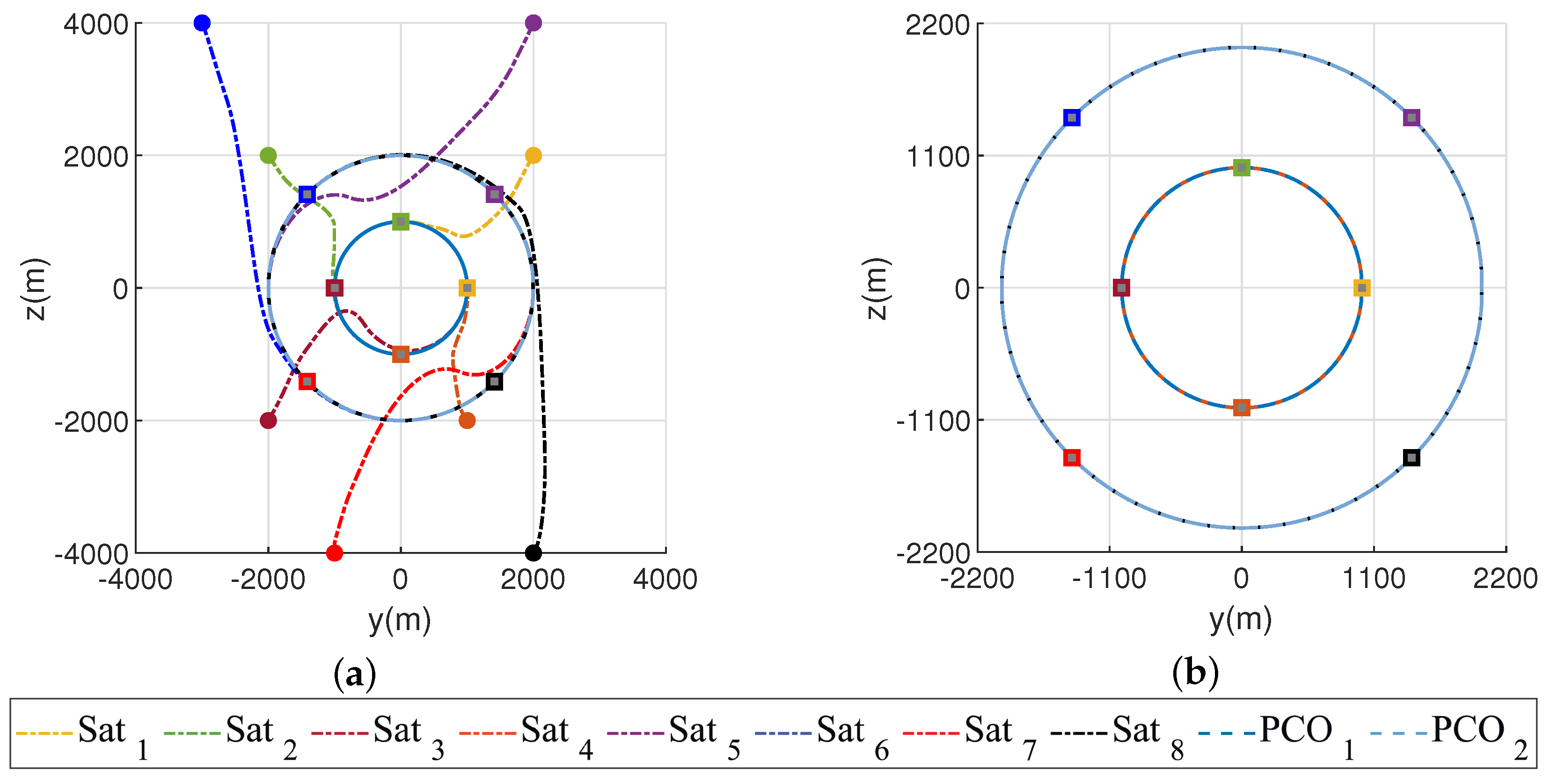
5. Projection Circular Orbits

When the master satellite moves in a circular Earth orbit, its angular acceleration is equal to zero [1]. In this case, it is valid for (1) that $\ddot{\theta }y=\ddot{\theta }x=0$, $r_c=const$, $\dot{\theta }=const=n$, where n is the average angular velocity of the master satellite, and Equations (1) and (2) are of the following form [35]:

$$\begin{array}{cc}& \ddot{x}-2n\dot{y}-n^{2}x=-{\displaystyle \frac{\mu (r_c+x)}{\gamma }}+\frac{\mu }{r_c^2}+a_x,\hfill \\ & \ddot{y}+2n\dot{x}-n^{2}y=-\frac{\mu y}{\gamma }+a_y,\hfill \\ & \ddot{z}=-{\displaystyle \frac{\mu z}{\gamma }}+a_z.\hfill \end{array}$$

(26)

Linearized equations of (26) are called the Hill–Clohessy–Wiltshire (HCW) equations [1,36]:

$$\begin{array}{cc}& \ddot{x}-2n\dot{y}-3n^{2}x=a_x,\hfill \\ & \ddot{y}+2n\dot{x}=a_y,\hfill \\ & \ddot{z}+n^{2}z=a_z.\hfill \end{array}$$

(27)

The HCW equations have the following limited periodic solutions [9]:

$$\left[\begin{array}{c}x\left(t\right)\\ y\left(t\right)\\ z\left(t\right)\end{array}\right]=\left[\begin{array}{c}\left(c_1/2\right)sin\left(nt+\varphi \right)\\ c_{1}cos\left(nt+\varphi \right)+c_3\\ c_{2}sin\left(nt+\varphi \right)\end{array}\right],$$

(28)

where x, y and z are the coordinates of the relative motion, $\varphi$ is the phase angle in the plane between the master satellite and the slave satellite (the initial phase angle is determined when the equator of the l master satellite’s in the locally horizontal plane $yz$) (the initial phase angle is defined, at the time of the equator crossing of the master satellite, in the local horizon $yz$ plane). Constants $c_1$, $c_2$, $c_3$, ${\alpha }_0$ are determined by the initial conditions as follows:

• The choice $c_1=c_2=\rho$, $c_3=0$ sets the configuration in which the slave satellite moves around the master satellite so that the projection of its movement on the local horizontal plane is the circle $y^2+z^2={\rho }^2$, where $\rho$ is a constant. Such an orbit is called a projection circular orbit (see Figure 2a).
• Selection $c_1=\rho$, $c_2={\displaystyle \frac{\sqrt{3}}{2}}$, $c_3=0$ sets the configuration in which the slave satellite moves around the master satellite in circles in the axes x, y and z of the local coordinate system: $x^2+y^2+z^2={\rho }^2$. This orbit is called the general circular orbit (GCO).
• Choice $c_1=c_2=0$, $c_3=\rho$ sets the master–slave or along-track orbit (ATO) configuration, where the slave satellite follows the master satellite along its orbit with a constant offset $\rho$ (see Figure 2b).

Substituting the values $c_1=c_2=r_{dpc}$, $c_3=0$ into equations (28), one obtains the following PCO equation:

$$\left[\begin{array}{c}{x}_d\left(t\right)\\ y_d\left(t\right)\\ z_d\left(t\right)\end{array}\right]=\left[\begin{array}{c}\left(r_{\mathrm{dpc}}/2\right)sin\left(nt+\varphi \right)\\ r_{\mathrm{dpc}}cos\left(nt+\varphi \right)\\ r_{\mathrm{dpc}}sin\left(nt+\varphi \right)\end{array}\right],$$

(29)

where $r_{\mathrm{dpc}}$ is the projected circular formation size, $\varphi$ is the in-plane phase angle between the master and the slave satellites, and n is the mean angular velocity, $n=\sqrt{\mu /a_c^3}$, where $a_c$ is the semi-major axis of the master satellite [1].

6. Control of PCO Constellation

Let the following aim of controlling a constellation of satellites be posed: there is a master satellite that moves in an elliptical orbit, but with a small eccentricity, i.e., its orbit is close to a circular orbit. It is necessary to create and maintain a certain constellation of satellites, which are located in a certain formation relative to the master satellite and keep this formation over time. In the case of a circular master satellite orbit, the most fuel-efficient slave satellite orbits would be general circular orbit (GCO), PCO, and along-track orbit (ATO) since such orbits are stable solutions of the HCW (27) equations. Then, control will be spent only on counteracting disturbances and countering unaccounted nonlinearities in the model (27).

The most interesting is the problem of positioning and maintaining the orbits of a constellation of satellites in the relative orbits of the PCO, even in the case of the master satellite’s elliptical orbits. It is also interesting to investigate the possibility of simultaneously storing a formation of a large number of satellites in different PCO orbits. In this variant set, several orbits have different $r_{dpc}$ in (29), and on the circles, the satellites are located with different offsets $\varphi$ so that a symmetric distribution of satellites is obtained.

To maintain the slave satellite position in the formation, it should use control law in the form of (25) where expressions (29) are used as the target path ${\mathbf{x}}_d\left(t\right)$. Configurable parameters are matrix $\mathbf{K}\in {\mathbb{R}}^{3\times 3}$ and vector $({\alpha }_1,{\alpha }_2,{\alpha }_3)$. A special case of the control law (25) is proportional-differential (PD) controllers of the following form:

$$\begin{array}{c}{\overline{u}}_x=-K_{px}{e}_x-K_{dx}{\dot{e}}_x\\ {\overline{u}}_y=-K_{py}{e}_y-K_{dy}{\dot{e}}_y\\ {\overline{u}}_z=-K_{pz}{e}_z-K_{dz}{\dot{e}}_z\end{array}$$

(30)

where $K_{px}$, $K_{dx}$, $K_{py}$, $K_{dy}$, $K_{pz}$, $K_{dz}$ are the positive adjustable gains. In the vector notation (30) can be written as

$$\overline{\mathbf{u}}=-{\mathbf{K}}_{\mathbf{pd}}\mathbf{e}$$

(31)

where matrix ${\mathbf{K}}_{\mathbf{pd}}\in {\mathbb{R}}^{3\times 6}$ has the following form

$$\begin{array}{c}\hfill {\mathbf{K}}_{\mathbf{pd}}=\left[\begin{array}{cccccc}{K}_{px}& 0& 0& K_{dx}& 0& 0\\ 0& K_{py}& 0& 0& K_{dy}& 0\\ 0& 0& K_{pz}& 0& 0& K_{dz}\end{array}\right].\end{array}$$

(32)

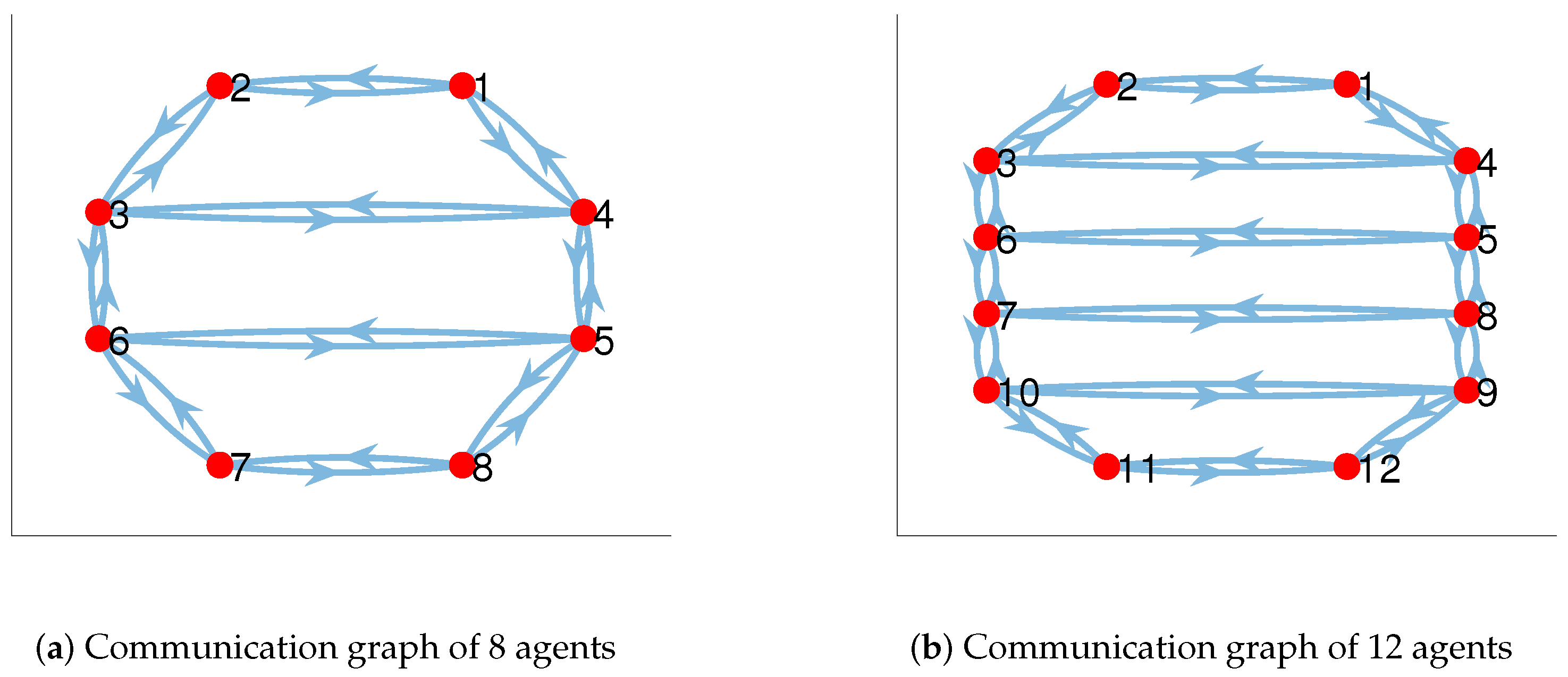
7. Multi-Agent Control and Consensus Algorithm

The obtained control laws (25) and (31) are applied separately to each satellite of the constellation and use information about the relative position in satellite form. To improve the accuracy of the formation positioning, you can apply multi-agent control based on the consensus algorithm (protocol) [37,38].

7.1. Basic Information on Consensus Algorithm

Graph $\mathcal{G}$ is a pair $(\mathcal{V},\mathcal{E})$, where $\mathcal{V}=1,\cdots ,n$ is a set of nodes (agents), $\mathcal{E}\in \mathcal{V}\times \mathcal{V}$ is a set of edges in which each edge is represented by an ordered pair of different nodes. Edge $(i,j)$ shows that node i is a neighboring to node j, and node j can receive information from node i. A graph is called undirected if for each $(i,j)\in \mathcal{E},(j,i)\in \mathcal{E}$. The path from node $i_1$ to node $i_l$ is a sequence of ordered edges of the form $(i_k,i_{k+1})$, $k=1,\cdots ,l-1$. An undirected graph is connected if for any $i\in \mathcal{V}$, there are paths to all other nodes.

Let graph $\mathcal{G}$ contain n nodes. The compatibility matrix $\mathcal{A}= \left[a_{ij}\right] \in {\mathbb{R}}^{n\times n}$ is defined as $a_{ii} = 0,a_{ij}=1$ if $(j,i)\in \mathcal{E}$, and 0 otherwise. The Laplace matrix $\mathcal{L} = \left[l_{ij}\right] \in {\mathbb{R}}^{n\times n}$ is defined as $l_{ii}={\sum }_{j=1}^N{a}_{ij}$ and $l_{ij}=-a_{ij},i\ne j$.

Let us assume that communication graph $\mathcal{G}$ is undirected and connected (some examples of undirected connected graphs are depicted in Figure 3). Assume that ${\xi }_i\in \mathbb{R}$ and ${\zeta }_i\in \mathbb{R}$ contain information about the state of the i-th agent. For information states with second-order dynamics, the following fundamental second-order consensus algorithm was proposed by Ren and Atkins in [39]:

$$\begin{array}{cc}& {\dot{\xi }}_i={\zeta }_i\hfill \\ & {\dot{\zeta }}_i=u_i\hfill \end{array}$$

(33)

where $u_i\in \mathbb{R}$ has the following form:

$$\begin{array}{c}\hfill u_i=-\sum _{j=1}^n{a}_{ij}\left({\gamma }_0\left({\xi }_i-{\xi }_j\right)+{\gamma }_1\left({\zeta }_i-{\zeta }_j\right)\right),\end{array}$$

(34)

where ${\gamma }_0>0,{\gamma }_1>0$.

For consensus algorithms (33) and (34), it is assumed that consensus is achieved asymptotically among several agents if for any ${\xi }_i\left(0\right)$ and ${\zeta }_i\left(0\right)$ it is valid that $∥{\xi }_i\left(t\right)-{\xi }_j\left(t\right)∥\to 0$ and $∥{\zeta }_i\left(t\right)-{\zeta }_j\left(t\right)∥\to 0$, for all $i\ne j$ as $t\to \infty$. In the case when ${\dot{\xi }}_i$ and ${\dot{\zeta }}_i$ represent the moving agent position and velocity, expression (34) defines its acceleration.

Denoting $\xi ={\left[{\xi }_1,\dots ,{\xi }_n\right]}^{\mathrm{T}}$ and $\zeta ={\left[{\zeta }_1,\dots ,{\zeta }_n\right]}^{\mathrm{T}}$, one can write the system model in the following vector form

$$\begin{array}{c}\hfill \left[\begin{array}{c}\dot{\xi }\hfill \\ \dot{\zeta }\hfill \end{array}\right]=\Gamma \left[\begin{array}{c}\xi \hfill \\ \zeta \hfill \end{array}\right]\end{array}$$

(35)

where

$$\begin{array}{c}\hfill \Gamma =\left[\begin{array}{cc}{0}_{n\times n}& I_n\\ -{\gamma }_0\mathcal{L}& -{\gamma }_1\mathcal{L}\end{array}\right]\end{array}$$

(36)

In the vector form, the control law is as

$$\begin{array}{c}\hfill U_c=-\left[{\gamma }_0\mathcal{L}\xi +{\gamma }_1\mathcal{L}\zeta \right]\end{array}$$

(37)

where $U_c\in {\mathbb{R}}^n$.

7.2. Consensus-Based Satellite Formation Control Law

The multi-agent satellite formation control law can be obtained by combining expressions (30) and (34). It should be noted that (34) is a control law for a single coordinate. Let us introduce the following notation: n is a number of agents in the formation (number of satellites); $i=1,\cdots ,n$ is the agent number; ${\mathbf{e}}_i={\left[\begin{array}{cccccc}{e}_{xi}& e_{yi}& e_{zi}& {\dot{e}}_{xi}& {\dot{e}}_{yi}& {\dot{e}}_{zi}\end{array}\right]}^{\mathrm{T}}$ is the error vector of i-th agent. Then the control law of agent i can be written as:

$$\begin{array}{cc}\hfill & {\overline{u}}_{xi}=-K_{px}{e}_{xi}-K_{dx}{\dot{e}}_{xi}-\sum _{j=1}^n{a}_{ij}\left({\gamma }_0\left(e_{xi}-e_{xj}\right)+{\gamma }_1\left({\dot{e}}_{xi}-{\dot{e}}_{xj}\right)\right),\hfill \\ \hfill & {\overline{u}}_{yi}=-K_{py}{e}_{yi}-K_{dy}{\dot{e}}_{yi}-\sum _{j=1}^n{a}_{ij}\left({\gamma }_0\left(e_{yi}-e_{yj}\right)+{\gamma }_1\left({\dot{e}}_{yi}-{\dot{e}}_{yj}\right)\right),\hfill \\ \hfill & {\overline{u}}_{zi}=-K_{pz}{e}_{zi}-K_{dz}{\dot{e}}_{zi}-\sum _{j=1}^n{a}_{ij}\left({\gamma }_0\left(e_{zi}-e_{zj}\right)+{\gamma }_1\left({\dot{e}}_{zi}-{\dot{e}}_{zj}\right)\right).\hfill \end{array}$$

(38)

Another variant of multi-agent control of the formation of satellites can be obtained based on (25). To do this, let us introduce the matrix of coefficients $\mathbf{K}={\left[\begin{array}{ccc}{\mathbf{k}}_x& {\mathbf{k}}_y& {\mathbf{k}}_z\end{array}\right]}^{\mathrm{T}}$, where ${\mathbf{k}}_x,{\mathbf{k}}_y,{\mathbf{k}}_z\in {\mathbb{R}}^{1\times 3}$, and vector $\mathbf{y}={\left[\begin{array}{ccc}{y}_x& y_y& y_z\end{array}\right]}^{\mathrm{T}}$. In new notations, (25) can be written as

$$\begin{array}{c}{\overline{u}}_x=-{\mathbf{k}}_x\mathbf{y},\\ {\overline{u}}_y=-{\mathbf{k}}_x\mathbf{y},\\ {\overline{u}}_z=-{\mathbf{k}}_x\mathbf{y}.\end{array}$$

(39)

Expressions (39) represent control vector components for a single agent. For the multi-agent control case, it is possible to employ the consensus algorithm for first-order systems since the combined output includes derivatives, and the zero-dynamics [31] of the system is stable. Then the control law based on the passivity of i-th agent can be written as:

$$\begin{array}{c}{\overline{u}}_{xi}=-{\mathbf{k}}_x{\mathbf{y}}_i-{\gamma }_0{\displaystyle \sum _{j=1}^n}{a}_{ij}(y_{xi}-y_{xj}),\\ {\overline{u}}_{yi}=-{\mathbf{k}}_y{\mathbf{y}}_i-{\gamma }_0{\displaystyle \sum _{j=1}^n}{a}_{ij}(y_{yi}-y_{yj}),\\ {\overline{u}}_{zi}=-{\mathbf{k}}_z{\mathbf{y}}_i-{\gamma }_0{\displaystyle \sum _{j=1}^n}{a}_{ij}(y_{zi}-y_{zj}).\end{array}$$

(40)

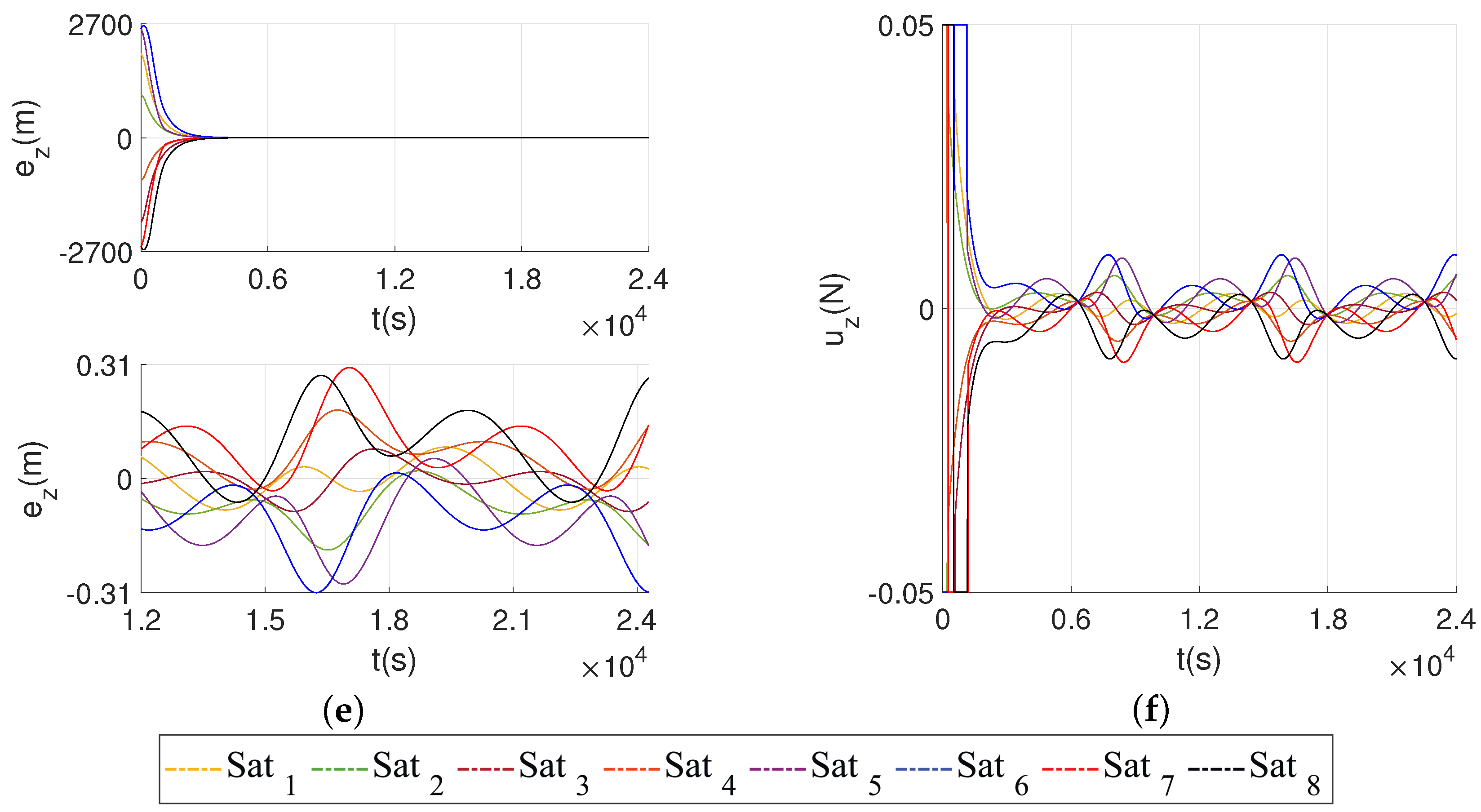
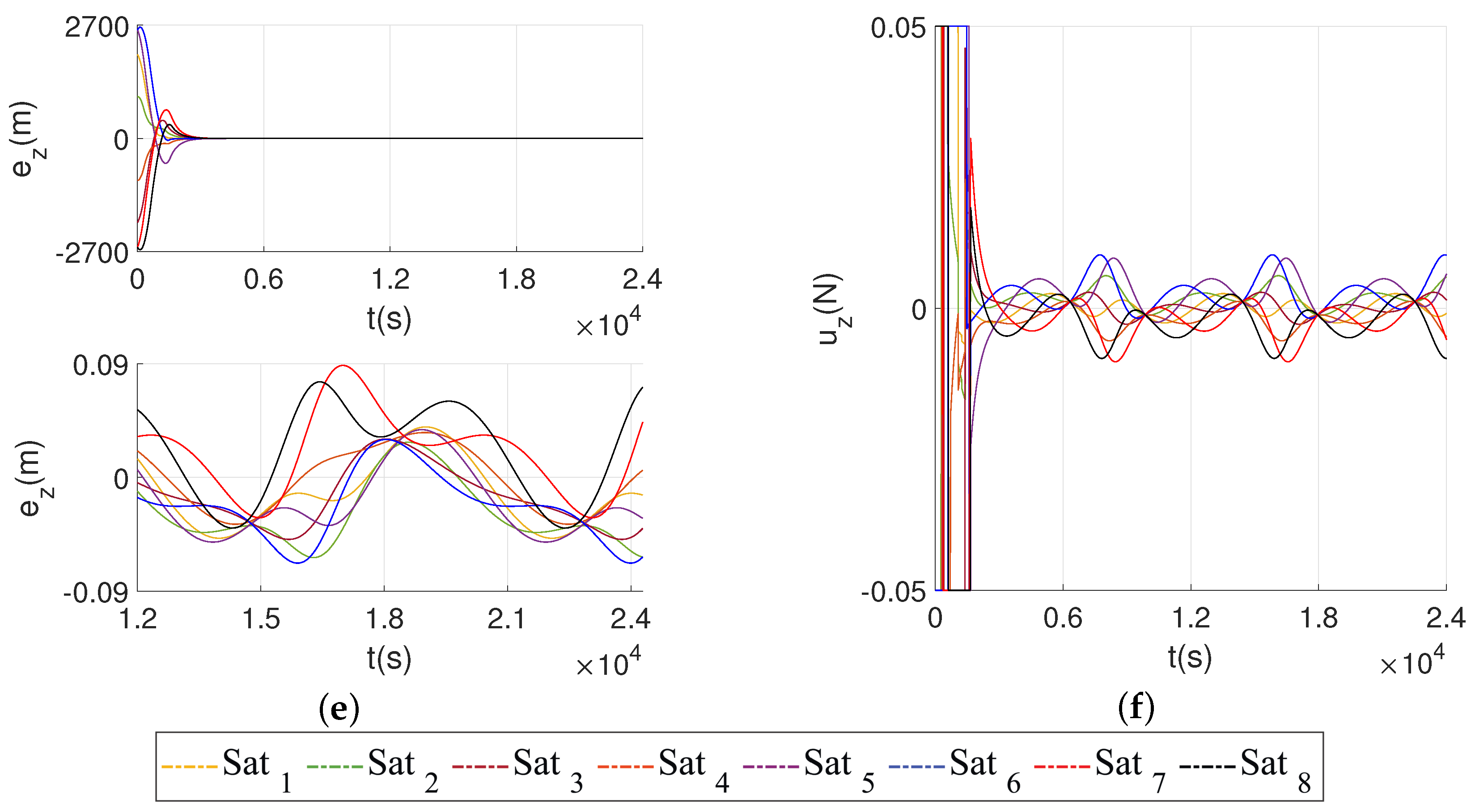
8. Simulation Results

For examining the developed control systems dynamics, a series of simulations was carried out in the MATLAB/Simulink software framework. The system considered was (1), (2) and four control laws, (25), (30), (38) and (40). In what follows, passification-based control (25) law control is denoted as PB law, law (30) is denoted as PD law, (38) as proportional-differential-consensus (PDC) law and (40) as passification-based consensus (PBC) law. One situation was simulated for all control laws: 8 satellites in two PCO orbits.

The leader’s satellite orbit was taken to be the same for all simulation runs. The leader’s orbit parameters are as follows: $m_F=10$ kg; ${\mu }_e=398.600$ km${}^3·{\mathrm{s}}^{-2}$; perigee radius $R_p=6971$ km; eccentricity $e=0.2$; $\Omega ,\omega =i=M=0$ rad/s. Disturbances $d_j\left(t\right)$ for $j=\{x,y,z\}$, acting on (1), (2), and including gravitational perturbations $J_2$, atmospheric resistance and solar radiation pressure perturbation forces were taken into account. The following disturbances model of [7,36] was adopted:

$$\left[\begin{array}{c}{d}_x\hfill \\ d_y\hfill \\ d_z\hfill \end{array}\right]=1.2\times {10}^{-3}\left[\begin{array}{c}1-1.5sin\left(nt\right)\\ 0.5sin\left(2nt\right)\\ sin\left(nt\right)\end{array}\right].$$

(41)

It is worth mentioning that model (41) gives the disturbances magnitudes which are slightly higher than the actual ones under the similar conditions.

8.1. Simulation for Motion of 8 Satellites in Two PCO Orbits

The radii of PCO orbits of 1000 m and 2000 m were set for the simulations. Each orbit contains four satellites. The phase shift between the agents located in the first orbit is $\pi /2$. The phase shift between small spacecraft located on the first orbit is as $\pi /2$, the second four, relative to the first $\pi /4$. The initial positions for 8 satellites are shown in

Table 1. Initial conditions for 8 satellites.

Satellite #	1	2	3	4	5	6	7	8
$X_x$ m	1000	666.7	−1000	−500	1000	−250	−666.7	500
$X_y$ m	2000	−2000	−2000	1000	2000	−3000	−1000	2000
$X_z$ m	2000	2000	−2000	−2000	4000	4000	−4000	−4000
${\dot{X}}_x$ m/s	0.0004	0.0004	0.0004	0.0004	0.0004	0.0004	0.0004	0.0004
${\dot{X}}_y$ m/s	0.0002	0.0002	−0.0002	0.0002	−0.0002	0.0004	−0.0002	−0.0005
${\dot{X}}_z$ m/s	0.0008	−0.0008	−0.0008	0.0008	0.0008	−0.0008	0.0008	−0.0008

.

8.2. Simulation the PD Laws and PDC Control Laws

The coefficients for the PD laws and PDC control laws (in SI units) are $K_{p_x}=K_{p_y}=K_{p_z}=0.025,K_{d_x}=K_{d_y}=K_{d_z}=15$. They are obtained by the trial-and-error method. The criterion is the positioning accuracy after two orbits around the Earth. For PDC, the consensus algorithm coefficients ${\gamma }_0=0.01$ and ${\gamma }_1=0.04$ were additionally set for the proportional and differential components, respectively. These coefficients are the same for the x, y, z channels of all 8 satellites. The communication graph is plotted in Figure 3a.

The simulation results for the flight of a group of 8 satellites with PD control are depicted in Figure 4 and Figure 5. The time histories of errors and control signals along x, y, z axes are shown in Figure 6. Figure 7 and Figure 8 demonstrate the simulation results of the motion of a group of 8 satellites with PDC control. The time histories of errors and control signals along x, y, z axes are shown in Figure 9.

Comparison of simulation results for PD and PDC laws is given in

Table 2. Position tracking errors for formation of 8 satellites.

Mode	${\mathit{e}}_{\mathit{x}}$, cm	${\mathit{e}}_{\mathit{y}}$, cm	${\mathit{e}}_{\mathit{z}}$, cm
PD	33	12	31
PDC	21	7.5	20
PB	23	9	23
PBC	11	4	9

.

8.3. Simulation the PB Laws and PBC Control Laws

The coefficients for the PB laws and PBC control laws (in SI units) are ${\alpha }_1 = {\alpha }_2={\alpha }_3=0.0025,{\mathbf{k}}_x = \left[\begin{array}{ccc}15& 1& 1\end{array}\right],{\mathbf{k}}_x = \left[\begin{array}{ccc}1& 15& 1\end{array}\right],{\mathbf{k}}_x = \left[\begin{array}{ccc}1& 1& 15\end{array}\right]$.

They are obtained by the trial-and-error method. The criterion is the positioning accuracy after two orbits around the Earth. For PBC, the consensus algorithm coefficients ${\gamma }_0=15.5$. These coefficients are the same for the x, y, z channels of all 8 satellites. The communication graph is plotted in Figure 3a. Figure 10 and Figure 11 show the simulation results of the flight of a group of 8 satellites with PB control. The time histories of errors and control signals along the axes x, y, z are depicted in Figure 12. Figure 13 and Figure 14 show the simulation results of the flight of a group of 8 satellites with PBC control. Time histories of errors and control signals along the axes x, y, z are shown in Figure 15.

Comparison of simulation results for PB and PBC algorithms for 8 satellites is demonstrated in Table 2.

9. Conclusions

In this paper, satellite formation reconfiguration and formation-keeping control laws are proposed by employing the passivity-based output feedback concept. For the complete nonlinear and time-dependent dynamics of the relative motion of a pair of satellites in elliptical orbits, new combined control algorithms, including a consensus protocol, are proposed and analyzed. A comparison of the control modes using passivity-based output feedback control and the proportional-differential controller with and without the consensus algorithm is given. The new result of the paper is also a rigorous mathematical proof of the use of control laws based on the passification method for the satellite system under consideration. The simplified version of the control law, which requires fewer calculations, is also considered. To increasing the accuracy of positioning satellites in the formation, in addition to the obtained algorithms, it is proposed to use multi-agent control algorithms based on the consensus protocol. Various methods of constructing satellite formations require the lowest energy costs to maintain the system. Mathematical modeling and computer simulations of the proposed algorithms for options for constructing formations are carried out in two PCO orbits of 8 satellites. The results obtained show good performance of the proposed satellites formation control laws for the problem of interest. It is demonstrated that the proposed formation-keeping control laws have robustness with respect to a variety of perturbations, including aspherical geopotential perturbation, air drag and solar radiation pressure.

References

1. Alfriend, K.; Vadali, S.; Gurfil, P. Spacecraft Formation Flying; Butterworth-Heinemann: Oxford, UK, 2010. [Google Scholar]
2. Mathavaraj, S.; Padhi, R. Satellite Formation Flying. High Precision Guidance using Optimal and Adaptive Control Techniques; Springer Nature: Singapore, 2021. [Google Scholar] [CrossRef]
3. Sengupta, P.; Vadali, S.; Alfriend, K. Modeling and control of satellite formations in high eccentricity orbits. J. Astronaut Sci. 2004, 52, 149–168. [Google Scholar] [CrossRef]
4. Wu, B.; Cao, X. Decentralized control for spacecraft formation in elliptic orbits. Aircr. Eng. Aerosp. Technol. 2017, 90, 166–174. [Google Scholar] [CrossRef]
5. Andrievsky, B.; Fradkov, A.L.; Kudryashova, E.V. Control of Two Satellites Relative Motion over the Packet Erasure Communication Channel with Limited Transmission Rate Based on Adaptive Coder. Electronics 2020, 9, 2032. [Google Scholar] [CrossRef]
6. Tirop, P.; Jingrui, Z. Review of Control Methods and Strategies of Space Tether Satellites. Am. J. Traffic Transp. Eng. 2019, 4, 137–148. [Google Scholar] [CrossRef]
7. Godard; Kumar, K. Fault Tolerant Reconfigurable Satellite Formations Using Adaptive Variable Structure Techniques. J. Guid. Control Dyn. 2010, 33, 969–984. [Google Scholar] [CrossRef]
8. Kim, D.; Woo, B.; Park, S.; Choi, K. Hybrid optimization for multiple-impulse reconfiguration trajectories of satellite formation flying. Life Sci. Space Res. 2009, 44, 1257–1269. [Google Scholar] [CrossRef]
9. Vaddi, S.S.; Alfriend, K.T.; Vadali, S.R.; Sengupta, P. Formation Establishment and Reconfiguration Using Impulsive Control. J. Guid. Control Dyn. 2005, 28, 262–268. [Google Scholar] [CrossRef]
10. Lim, H.C.; Bang, H.C. Trajectory Planning of Satellite Formation Flying using Nonlinear Programming and Collocation. J. Astron. Space Sci. 2008, 25, 361–374. [Google Scholar] [CrossRef]
11. Eyer, J. A Dynamics and Control Algorithm for Low Earth Orbit Precision Formation Flying Satellites. Ph.D. Thesis, Graduate Department of Aerospace Science and Engineering, University of Toronto, Toronto, ON, Canada, 2009. [Google Scholar]
12. Bonin, G.; Roth, N.; Armitage, S.; Newman, J.; Risi, B.; Zee, R. Can-4 and CanX-5 Precision Formation Flight: Mission Accomplished! In Proceedings of the 29th Annual AIAA/USU Conference on Small Satellites, Logan, UT, USA, 8–13 August 2015; Univ. of Toronto Inst. for Aerospace Studies: Toronto, ON, Canada, 2015. [Google Scholar]
13. Ulrich, S. Nonlinear passivity-based adaptive control of spacecraft formation flying. Am. Control. Conf. 2016, 7432–7437. [Google Scholar] [CrossRef]
14. de Queiroz, M.S.; Kapila, V.; Yan, Q. Adaptive Nonlinear Control of Multiple Spacecraft Formation Flying. J. Guid. Control Dyn. 2000, 23, 385–390. [Google Scholar] [CrossRef]
15. Wong, H.; Kapila, V.; Sparks, A. Adaptive output feedback tracking control of multiple spacecraft. In Proceedings of the 2001 American Control Conference (Cat. No.01CH37148), Arlington, VA, USA, 25–27 June 2001; Volume 2, pp. 698–703. [Google Scholar] [CrossRef]
16. Shahid, K.; Kumar, K. Satellite formation flying using variable structure model reference adaptive control. Proc. Inst. Mech. Eng. Part G—J. Aerosp. Eng. 2009, 223, 271–283. [Google Scholar] [CrossRef]
17. Zou, A.M.; Kumar, K.D. Distributed Attitude Coordination Control for Spacecraft Formation Flying. IEEE Trans. Aerosp. Electron. Syst. 2012, 48, 1329–1346. [Google Scholar] [CrossRef]
18. Leonard, C.L.; Hollister, W.M.; Bergmann, E.V. Orbital formationkeeping with differential drag. J. Guid. Control Dyn. 1989, 12, 108–113. [Google Scholar] [CrossRef]
19. Bevilacqua, R.; Hall, J.; Romano, M. Multiple spacecraft rendezvous maneuvers by differential drag and low thrust engines. Celest. Mech. Dyn. Astron. 2010, 106, 69–88. [Google Scholar] [CrossRef]
20. Bevilacqua, R.; Romano, M. Rendezvous Maneuvers of Multiple Spacecraft Using Differential Drag Under J2 Perturbation. J. Guid. Control Dyn. 2008, 31, 1595–1607. [Google Scholar] [CrossRef] [Green Version]
21. Shirobokov, M.; Trofimov, S. Formation control in low-earth orbits by means of machine learning methods. Prepr. Keldysh Inst. 2020, 19, 1–32. (In Russian) [Google Scholar] [CrossRef]
22. Shirobokov, M.; Trofimov, S.; Ovchinnikov, M. Survey of machine learning techniques in spacecraft control design. Acta Astronaut. 2021, 186, 87–97. [Google Scholar] [CrossRef]
23. Andrievsky, B.; Kuznetsov, N.; Popov, A. Algorithms for aerodynamic control of relative motion two satellites in a near circular orbit. Differ. Equ. Control Process. 2020, 4, 28–58. (In Russian) [Google Scholar]
24. Baranov, A.; Chernov, N. Energy cost analysis to station keeping for satellite formation type “TerraSAR-X—TanDEM-X”. Rudn. J. Eng. Res. 2019, 20, 220–228. [Google Scholar] [CrossRef] [Green Version]
25. Baranov, A.; Baranov, A. Maintenance of Preset Configuration of a Satellite Constellation. Kosm. Issled. 2009, 47, 48–54. [Google Scholar]
26. Gunchenko, M.; Ulybyshev, Y. Long-term linear-quadratic control of satellite constellations in highly elliptical orbits. J. Comput. Syst. Sci. Int. 2018, 57, 482–493. [Google Scholar] [CrossRef]
27. Vaddi, S. Modeling and Control of Satellite Formations. Ph.D. Thesis, Department of Aerospace Engineering, Texas A&M University, College Station, TX, USA, 2003. [Google Scholar]
28. Ivanov, D.; Monakhova, U.; Ovchinnikov, M. Nanosatellites swarm deployment using decentralized differential drag-based control with communicational constraints. Acta Astronaut. 2019, 159, 646–657. [Google Scholar] [CrossRef]
29. Scharnagl, J.; Kempf, F.; Schilling, K. Combining Distributed Consensus with Robust H∞-Control for Satellite Formation Flying. Electronics 2019, 8, 319. [Google Scholar] [CrossRef] [Green Version]
30. Park, H.E.; Park, S.Y.; Choi, K.H. Satellite formation reconfiguration and station-keeping using state-dependent Riccati equation technique. Aerosp. Sci. Technol. 2011, 15, 440–452. [Google Scholar] [CrossRef]
31. Khalil, H.K. Nonlinear Systems, 3rd ed.; Prentice-Hall: Upper Saddle River, NJ, USA, 2002. [Google Scholar]
32. Fradkov, A.L.; Druzhinina, M.V. Reduced order shunt nonlinear adaptive controller. In Proceedings of the 1997 European Control Conference (ECC), Brussels, Belgium, 1–4 July 1997; pp. 1231–1236. [Google Scholar]
33. Andrievsky, B.; Fradkov, A. Method of passification in adaptive control, estimation, and synchronization. Autom. Remote Control 2006, 67, 1699–1731. [Google Scholar] [CrossRef]
34. Barkana, I. Output feedback stabilizability and passivity in nonstationary and nonlinear systems. Int. J. Adapt. Control. Signal Process. 2010, 24, 568–591. [Google Scholar] [CrossRef]
35. Vaddi, S.; Alfriend, K.; Vadali, S. Formation Flying: Accommodating Nonlinearity and Eccentricity Perturbations. J. Guid. Control Dyn. 2003, 26, 214–223. [Google Scholar] [CrossRef]
36. Chobotov, V. Orbital Mechanics; AIAA Education Series; American Institute of Aeronautics & Astronautics: Reston, VA, USA, 2002. [Google Scholar]
37. Ren, W.; Beard, R.W. Distributed Consensus in Multi-Vehicle Cooperative Control; Springer: London, UK, 2008. [Google Scholar] [CrossRef]
38. Olfati-Saber, R.; Murray, R. Consensus problems in networks of agents with switching topology and time-delays. IEEE Trans. Automat. Control 2004, 49, 1520–1533. [Google Scholar] [CrossRef] [Green Version]
39. Ren, W.; Atkins, E. Distributed multi-vehicle coordinated control via local information exchange. Int. J. Robust Nonlinear Control 2007, 17, 1002–1033. [Google Scholar] [CrossRef] [Green Version]
Figure 1. Reference systems.
Electronics 10 03111 g001
Figure 2. Configurations of satellite orbits. (a) Projected circular orbit. (b) Along-track orbit.
Electronics 10 03111 g002
Figure 3. Examples of communication graphs of 8 and 12 agents.
Electronics 10 03111 g003
Figure 4. PD law: Plot of 3D trajectory.
Electronics 10 03111 g004
Figure 5. PD law. Trajectories plots: (a) on plane YZ; (b) on plane YZ after orbiting.
Electronics 10 03111 g005
Figure 6. PD law. Error and control time histories: (a) errors along axis x; (b) controls along axis x; (c) errors along y; (d) controls along y; (e) errors along axis z; (f) control along axis z.
Electronics 10 03111 g006aElectronics 10 03111 g006b
Figure 7. PDC law: Plot of 3D trajectory.
Electronics 10 03111 g007
Figure 8. PDC law. Trajectories’ plots: (a) on plane YZ; (b) on plane YZ after orbiting.
Electronics 10 03111 g008
Figure 9. PDC law. Error and control time histories: (a) errors along axis x; (b) controls along axis x; (c) errors along axis y; (d) controls along axis y; (e) errors along axis z; (f) control along axis z.
Electronics 10 03111 g009aElectronics 10 03111 g009b
Figure 10. PB law. Plot of 3D trajectory.
Electronics 10 03111 g010
Figure 11. PB law. Plots of trajectories: (a) on plane YZ; (b) on plane YZ after orbiting.
Electronics 10 03111 g011
Figure 12. PB law. Error and control time histories: (a) errors along axis x; (b) controls along axis x; (c) errors along axis y; (d) controls along axis y; (e) errors along axis z; (f) control along axis z.
Electronics 10 03111 g012aElectronics 10 03111 g012b
Figure 13. PBC law. Plot of 3D trajectory.
Electronics 10 03111 g013
Figure 14. PBC law. Plots of trajectories: (a) on plane YZ; (b) on plane YZ after orbiting.
Electronics 10 03111 g014
Figure 15. PBC law. Error and control time histories: (a) errors along axis x; (b) controls along axis x; (c) errors along axis y; (d) controls along axis y; (e) errors along axis z; (f) control along axis z.
Electronics 10 03111 g015aElectronics 10 03111 g015b