Article

EWOA-OPF: Effective Whale Optimization Algorithm to Solve Optimal Power Flow Problem

by
Mohammad H. Nadimi-Shahraki
1,2,*,
Shokooh Taghian
1,2,
Seyedali Mirjalili
3,4,*,
Laith Abualigah
5,6,
Mohamed Abd Elaziz
7,8,9,10 and
Diego Oliva
11
1
Faculty of Computer Engineering, Najafabad Branch, Islamic Azad University, Najafabad 8514143131, Iran
2
Big Data Research Center, Najafabad Branch, Islamic Azad University, Najafabad 8514143131, Iran
3
Centre for Artificial Intelligence Research and Optimisation, Torrens University Australia, Brisbane, QLD 4006, Australia
4
Yonsei Frontier Lab, Yonsei University, Seoul 03722, Korea
5
Faculty of Computer Sciences and Informatics, Amman Arab University, Amman 11953, Jordan
6
School of Computer Sciences, University Sains Malaysia, Gelugor 11800, Malaysia
7
Department of Mathematics, Faculty of Science, Zagazig University, Zagazig 44519, Egypt
8
Artificial Intelligence Research Center (AIRC), Ajman University, Ajman 346, United Arab Emirates
9
Department of Artificial Intelligence Science & Engineering, Galala University, Suez 435611, Egypt
10
School of Computer Science and Robotics, Tomsk Polytechnic University, 634050 Tomsk, Russia
11
Departamento de Innovación Basada en la Información y el Conocimiento, Universidad de Guadalajara, CUCEI, Guadalajara 44430, Mexico
*
Authors to whom correspondence should be addressed.
Electronics 2021, 10(23), 2975; https://doi.org/10.3390/electronics10232975
Submission received: 25 October 2021 / Revised: 20 November 2021 / Accepted: 26 November 2021 / Published: 29 November 2021
(This article belongs to the Special Issue Big Data Analytics Using Artificial Intelligence)

Abstract

:
The optimal power flow (OPF) is a vital tool for optimizing the control parameters of a power system by considering the desired objective functions subject to system constraints. Metaheuristic algorithms have been proven to be well-suited for solving complex optimization problems. The whale optimization algorithm (WOA) is one of the well-regarded metaheuristics that is widely used to solve different optimization problems. Despite the use of WOA in different fields of application as OPF, its effectiveness is decreased as the dimension size of the test system is increased. Therefore, in this paper, an effective whale optimization algorithm for solving optimal power flow problems (EWOA-OPF) is proposed. The main goal of this enhancement is to improve the exploration ability and maintain a proper balance between the exploration and exploitation of the canonical WOA. In the proposed algorithm, the movement strategy of whales is enhanced by introducing two new movement strategies: (1) encircling the prey using Levy motion and (2) searching for prey using Brownian motion that cooperate with canonical bubble-net attacking. To validate the proposed EWOA-OPF algorithm, a comparison among six well-known optimization algorithms is established to solve the OPF problem. All algorithms are used to optimize single- and multi-objective functions of the OPF under the system constraints. Standard IEEE 6-bus, IEEE 14-bus, IEEE 30-bus, and IEEE 118-bus test systems are used to evaluate the proposed EWOA-OPF and comparative algorithms for solving the OPF problem in diverse power system scale sizes. The comparison of results proves that the EWOA-OPF is able to solve single- and multi-objective OPF problems with better solutions than other comparative algorithms.

1. Introduction

Over the past decades, metaheuristic algorithms (MAs) have become more prevalent in solving optimization problems in various fields of industry and science [1]. The widespread usage of MAs for solving different optimization problems verified their ability for solving complex problems with difficulties such as non-linear constraints, multi-modality of the problem, and a non-convex search landscape [1,2]. Metaheuristics are a class of general-purpose stochastic algorithms that can be applied to any optimization problem [3]. Despite exact algorithms, metaheuristics allow tackling complex problems by providing satisfactory solutions in a reasonable time [4]. MAs estimate the approximate optimal solution of the problem by sampling the solution space to find or generate better solutions. Many combinatorial optimization problems were solved using metaheuristic algorithms in diverse engineering fields such as civil, mechanical, electrical, industrial, and system engineering. Several new optimization algorithms have been proposed recently due to the emergence of the no free lunch (NFL) theorem [5], which states that no particular optimization algorithm can solve all problems of all kinds of complexities. It is also discovered that using the same algorithm on the same problem yields varied results depending on the various parameter settings.
The inspiration and imitation of creatures’ behaviors led to many effective metaheuristics to find the optimum solution for different problems. The MAs based on their source of inspiration can be broadly classified into two main categories: evolutionary and swarm intelligence algorithms. The algorithms that imitate an evolutionary phenomenon in nature are classified as evolutionary algorithms. These algorithms improve a randomly generated population of solutions for a particular optimization problem by employing evolutionary principles. Genetic algorithm (GA) [6], genetic programming (GP) [7], evolution strategy (ES) [8], evolutionary programming (EP) [9], and differential evolution (DE) [10] are the most well-known algorithms in this category. Swarm intelligence algorithms mimic simple behaviors of social creatures in which the individuals cooperate and interact collectively to find promising regions. Some of the best known and recently proposed swarm intelligence algorithms are particle swarm optimization (PSO) [11], the bat algorithm (BA) [12], krill herd (KH) [13], the grey wolf optimizer (GWO) [14], the whale optimization algorithm (WOA) [15], the salp swarm algorithm (SSA) [16], the squirrel search algorithm (SSA) [17], the African vultures optimization algorithm (AVOA), and the Aquila optimizer (AO) [18] algorithm.
On the other hand, the optimal power flow (OPF) is a non-linear and non-convex problem that is considered one of the power system’s complex optimization problems [19]. OPF adjusts both continuous and discrete control variables to optimize specified objective functions by satisfying the operating constraints [20]. From the perspective of industries and power companies, minimizing the operational cost and maximizing the reliability of power systems are two primary objectives. Since a slight modification in power flow can considerably raise the running expense of power systems, the OPF focuses on the economic aspect of operating power systems [21]. Non-linear programming [22], Newton algorithm [23], and quadratic programming [24] are some of the classical optimization algorithms that have been employed to tackle the OPF problem. Although these algorithms can sometimes find the global optimum solution, they have some drawbacks such as getting trapped in local optima, a high sensitivity to initial potions, and the inability to deal with non-differentiable objective functions [25,26,27]. Thus, it is essential to develop effective optimization algorithms to overcome these shortcomings and deal with such challenges efficiently.
Regarding MA, the whale optimization algorithm (WOA) is a swarm-based algorithm inspired by the hunting behavior of humpback whales in nature. The humpback whales use the bubble-net hunting technique to encircle and catch their prey that are in collections of fishes close to water level. The whales go down the surface and dive into the prey, then swarm in a spiral-shaped path while they start creating bubbles. The whales’ spiral movement radius narrows when prey get closer to the surface, enabling them to attack. WOA consists of three phases: encircling the prey, bubble-net attacking, and searching for the prey. WOA has been used to solve a wide range of optimization problems in different applications including feature selection [28], software defect prediction [29], clustering [30,31], classification [32,33], disease diagnosis [34], image segmentation [35,36], scheduling [37], forecasting [38,39], parameter estimation [40], global optimization [41], and photovoltaic energy generation systems [42,43]. Even though WOA is employed to tackle a wide variety of optimization problems, it still has flaws such as premature convergence, the imbalance between exploration and exploitation, and local optima stagnation [44,45].
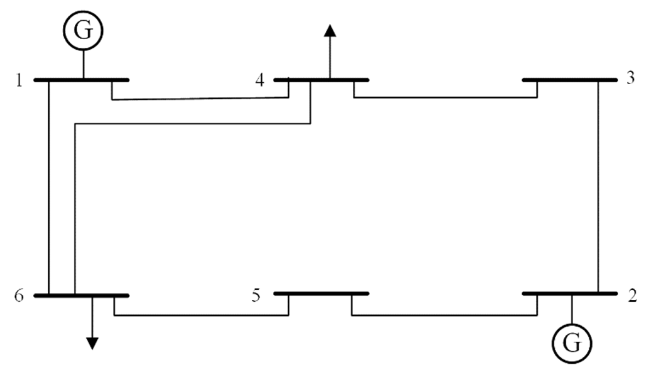
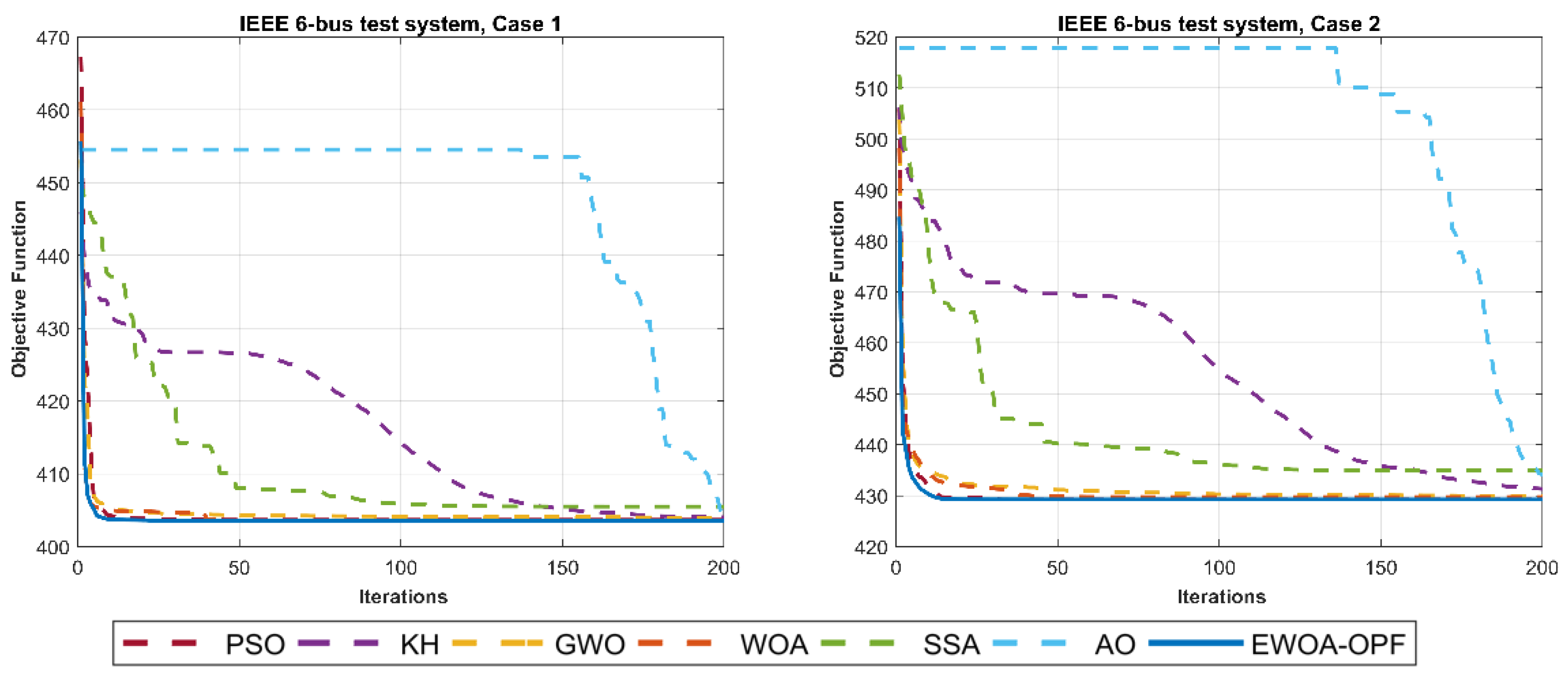
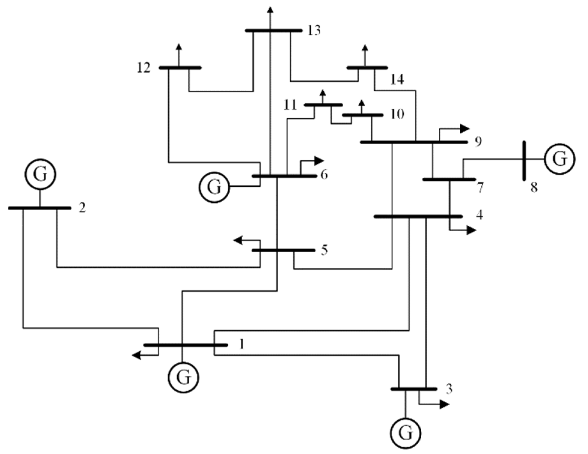
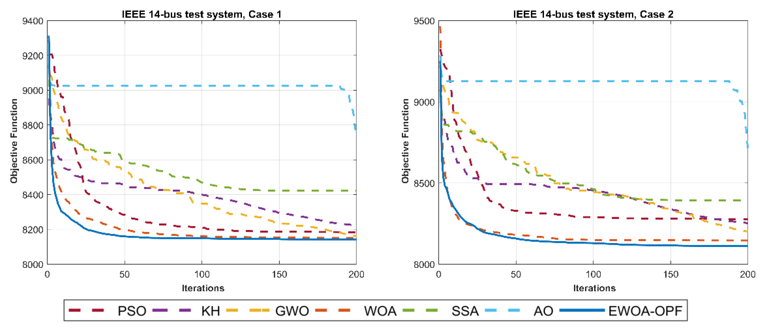
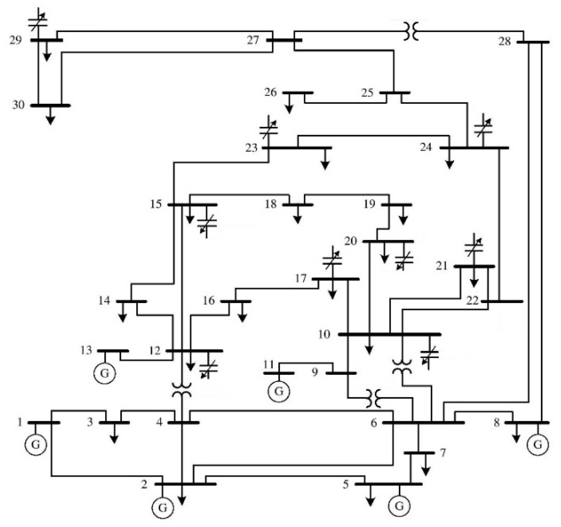
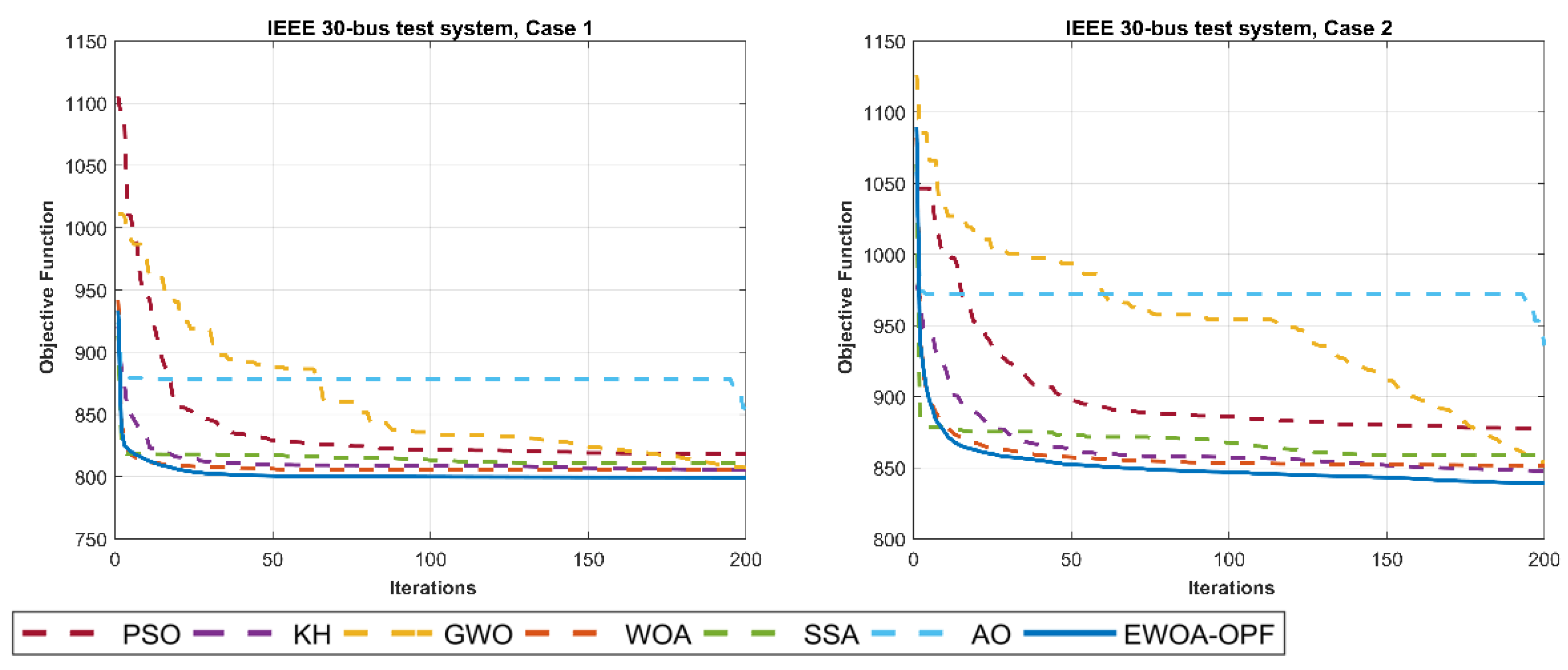
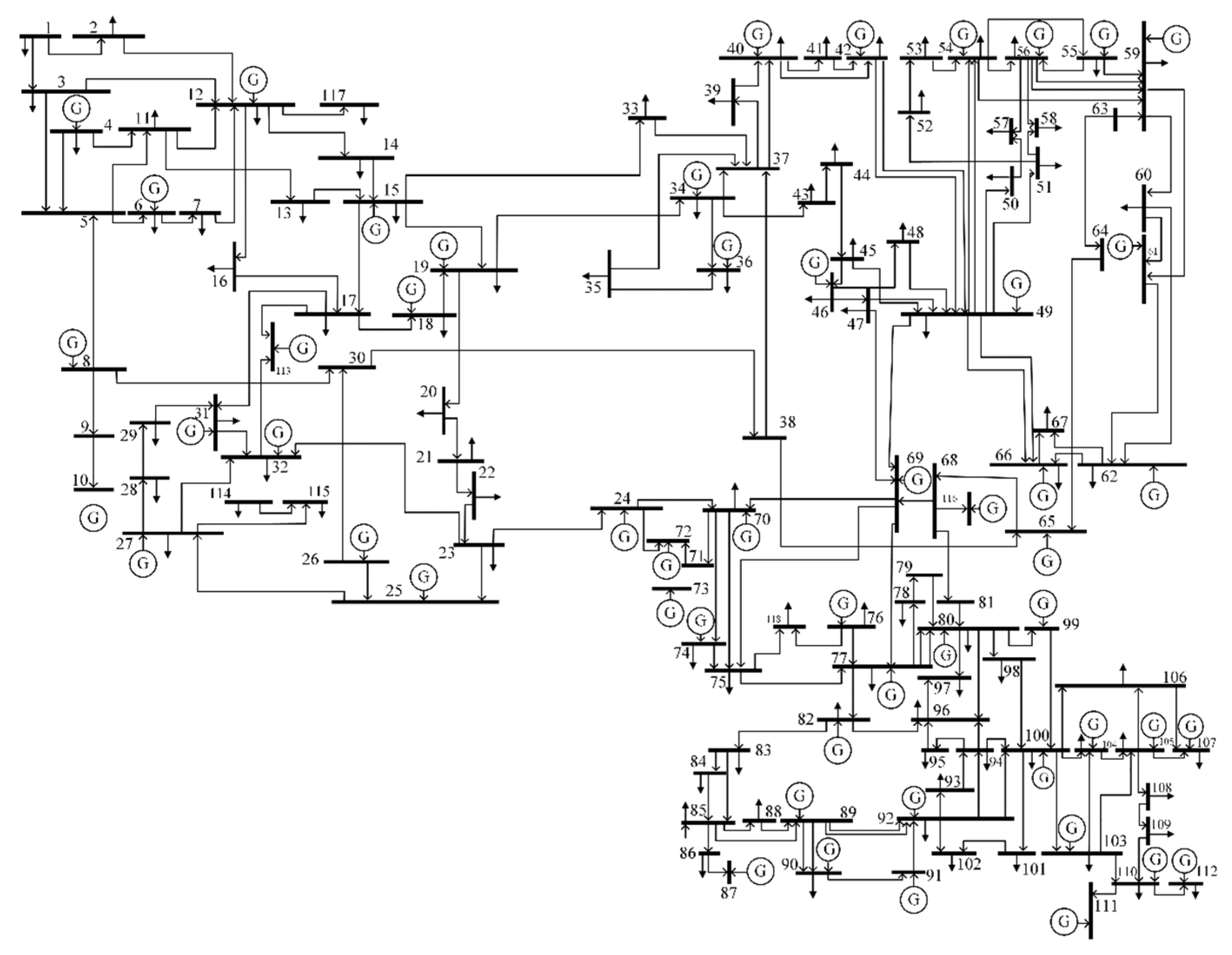
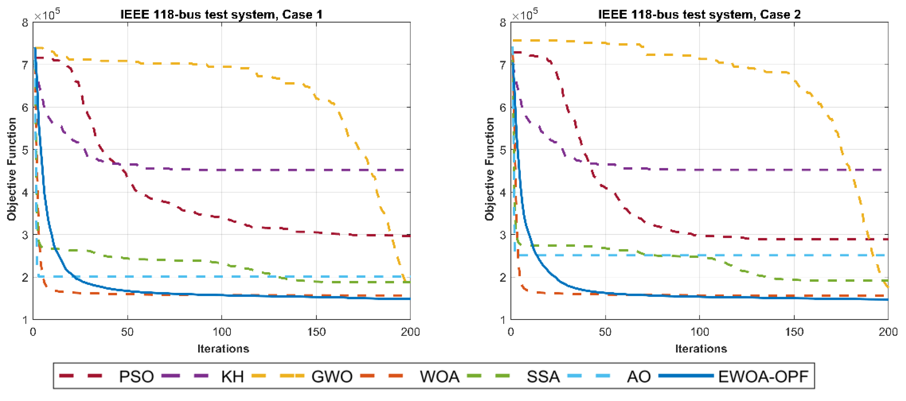
This paper proposes an effective whale optimization algorithm for solving the optimal power flow problem (EWOA-OPF). The EWOA-OPF improves the movement strategy of whales by introducing two new movement strategies: (1) encircling the prey using Levy motion and (2) searching for prey using Brownian motion that cooperate with canonical bubble-net attacking. The reason for these changes is to maintain an appropriate balance between exploration and exploitation and enhance the exploration ability of the WOA, resulting in more precise solutions when solving problems. To validate the proposed EWOA-OPF algorithm, a comparison among well-known optimization algorithms is established under single- and multi-objective functions of the OPF. Standard IEEE 6-bus, IEEE 14-bus, IEEE 30-bus, and IEEE 118-bus test systems are used to evaluate the proposed EWOA-OPF and comparative algorithms for solving OPF problems in diverse power system scale sizes. The results were compared with four state-of-the-art algorithms consisting of particle swarm optimization (PSO) [11], krill herd (KH) [13], the grey wolf optimizer (GWO) [14], and the whale optimization algorithm (WOA) [15] and two recently proposed algorithms, the salp swarm algorithm (SSA) [16] and the Aquila optimizer (AO) [18] algorithm. The comparison of results proves that the EWOA-OPF can solve single- and multi-objective OPF problems with better solutions than other comparative algorithms.
The rest of the paper is organized as follows: the related works are reviewed in Section 2. Section 3 presents the OPF problem formulation and objective functions. Section 4 contains the mathematical model of WOA. Section 5 presents the proposed EWOA-OPF. The experimental evaluation of EWOA-OPF and comparative algorithms on OPF is presented in Section 6. Finally, the conclusion and future work are given in Section 7.

2. Related Work

The purpose of optimization is to find the global optimum solution among numerous candidate solutions. Traditional optimization methods have several drawbacks when solving complex and complicated problems that require considerable time and cost optimization. Metaheuristic algorithms have been proven capable of handling a variety of continuous and discrete optimization problems [46] in a wide range of applications including engineering [47,48,49], industry [50,51], image processing and segmentation [52,53,54], scheduling [55,56], photovoltaic modeling [57,58], optimal power flow [59,60], power and energy management [61,62], planning and routing problems [63,64,65], intrusion detection [66,67], feature selection [68,69,70,71,72], spam detection [73,74], medical diagnosis [75,76,77], quality monitoring [78], community detection [79], and global optimization [80,81,82]. In the following, some representative metaheuristic algorithms from the swarm intelligence category used in our experiments are described. Then, some metaheuristic algorithms were used to solve OPF are highlighted.
Swarm intelligence algorithms mimic the collective behavior of creatures in nature such as birds, fishes, wolves, and ants. The main principle of these algorithms is to deal with a population of particles that can interact with each other. Eberhart and Kennedy proposed the particle swarm optimization (PSO) [11] method, which simulates bird flocks’ foraging and navigation behavior. It is derived from basic laws of interaction amongst birds, which prefer to retain their flight direction considering their current direction, the local best position gained so far, and the global best position that the swarm has discovered thus far. The PSO algorithm concurrently directs the particles to the best optimum solutions by each individual and the swarm. The krill herd (KH) [13] algorithm is a population-based metaheuristic algorithm based on the krill individual herding behavior modeling. The KH algorithm repeats the three motions and searches in the same direction until it finds the optimum answer. Other krill-induced movements, foraging activity, and random diffusion all have an impact on the position.
Another well-known swarm intelligence algorithm is the grey wolf optimizer (GWO) [14], which is inspired by grey wolves in nature that look for the best approach to pursue prey. In nature, the GWO algorithm uses the same method, following the pack hierarchy to organize the wolves’ pack’s various responsibilities. GWO divides pack members into four divisions depending on each wolf’s involvement in the hunting process. The four groups are alpha, beta, delta, and omega, with alpha being the finest hunting solution yet discovered. The salp swarm algorithm (SSA) [16] is another recent optimizer that is based on natural salp swarm behavior. As a result, it creates and develops a set of random individuals within the problem’s search space. Following that, the chain’s leader and followers must update their location vectors. The leader salp will assault in the direction of a food supply, while the rest of the salps can advance towards it. The Aquila optimizer (AO) [18] is one of the latest proposed algorithms in the swarm intelligence category that simulates the prey-catching behavior of Aquila in nature. In AO, four methods were used to emulate this behavior consisting of selecting the search space by a high soar with a vertical stoop, exploring within a diverge search space by contour flight with short glide attack, exploiting within a converge search space by low flight with slow descent attack, and swooping by walk and grab prey.
Regardless of the nature of the algorithm, the majority of the metaheuristics, especially the population-based algorithms, have two standard contrary criteria in the search process: the exploration of the search space and the exploitation of the gained best solutions. In exploitation, the promising regions are explored more thoroughly for generating similar solutions to improve the previously obtained solution. In exploration, non-explored regions must be visited to be sure that all regions of the search space are evenly explored and that the search is not only limited to a reduced number of regions. Excessive exploitation decreases diversity and leads to premature convergence, whereas excessive exploration leads to gradual convergence [83]. Thus, metaheuristic algorithms try to balance between the exploration and exploitation that has a crucial impact on the performance of the algorithm and the gained solution [84]. Furthermore, real-world problems require achieving several objectives that are in conflict with one another such as minimizing risks, maximizing reliability, and minimizing cost. There is only one objective function to be optimized and only one global solution to be found in a single-objective problem. However, in multi-objective problems, as there is no single best solution, the aim is to find a set of solutions representing the trade-offs among the different objectives [85].
Although metaheuristic algorithms have several merits over classical optimization algorithms, such as the simple structure, independence to the problem, the gradient-free nature, and finding near-global solutions [14], they may encounter premature convergence, local optima entrapment, and the loss of diversity. In this regard, improved variants of these algorithms have been proposed, each of which adapted to tackle such weaknesses [86,87,88]. Additionally, the significant growth of metaheuristic algorithms has resulted in a trend of solving OPF problems by using population-based metaheuristic algorithms. In the literature, the OPF was solved by using black hole (BO) [89], teaching–learning based optimization (TLBO) [90] algorithms, the krill herd (KH) algorithm [91], the equilibrium optimizer (EO) algorithm [92], and the slime mould algorithm (SMA) [93]. Additionally, some studies used the modified and enhanced version of the canonical swarm intelligence algorithms for solving OPF with different test systems such as the modified shuffle frog leaping algorithm (MSLFA) for multi-objective optimal power flow [94] that added a mutation strategy to overcome the problem of being trapped in local optima.
Another work proposed an improved grey wolf optimizer (I-GWO) [95] to improve the GWO search strategy with a dimension learning-based hunting search strategy to deal with exploration and exploitation imbalances and premature convergence weaknesses. In [96], quasi-oppositional teaching–learning based optimization (QOTLBO) proposed to improve the convergence speed and quality of obtained solutions by using quasi-oppositional based learning (QOBL). In [97], particle swarm optimization with an aging leader and challengers (ALC-PSO) algorithm was applied to solve the OPF problem by using the concept of the leader’s age and lifespan. The aging mechanism can avoid the premature convergence of PSO and result in better convergence. An improved artificial bee colony optimization algorithm was based on orthogonal learning (IABC) [98] to adjust exploration and exploitation. In [99], the modified sine–cosine algorithm (MSCA) was aimed to reduce the computational time with sufficient improvement in finding the optimal solution and feasibility. The MSCA benefits from using Levy flights cooperated by the strategy of the canonical sine–cosine algorithm to avoid local optima. In the high-performance social spider optimization algorithm (NISSO) [100], the canonical SSO algorithm was modified by using two new movement strategies that resulted in faster convergence to the optimal solution and finding better solutions in comparison to comparative algorithms.

3. OPF Problem Formulation and Objective Functions

The optimal power flow (OPF) is regarded as a fundamental tool for the effective design and operation of the power networks. The main aim of OPF is to find the optimum values of control variables for different objective functions while satisfying the system equality and inequality constraints within the permitted boundaries. The mathematical formulation and description of OPF single- and multi-objective functions are presented in detail as follows.

3.1. OPF Problem Formulation

The OPF is a non-linear and non-convex optimization problem that aims to find the best set of the power system’s control variables and satisfy the desired objective function. The OPF problem is mathematically formulated [101] as shown in Equation (1):
M i n   F ( x , u ) S u b j e c t   t o :   g ( x , u ) = 0 , h ( x , u ) 0 ,
where F is the objective function to be minimized, x is the vector of dependent (state) variables, u is the vector of independent (control) variables, and g and h represent equality and inequality constraints, respectively. Accordingly, vector x, which consists of slack bus power PG1, load bus voltage VL, generator reactive power output QG, and transmission line loading Sl, is presented by Equation (2),
x = [ P G 1 , V L 1 , , V L N L , Q G 1 , , Q G N G , S l 1 , , S l N T L ]
where NL, NG, and NTL are the number of load buses, number of generators, and number of transmission lines, respectively. u is the vector of control variables, consisting of generator active power outputs PG (except at the slack bus PG1), generator voltages VG, transformer tap settings T, and shunt VAR compensations QC, which is presented as Equation (3),
u = [ P G 2 , , P G N G , V G 1 , , V G N G , T 1 , , T N T , Q C 1 , , Q C N C ]
where NT and NC are the number of the regulating transformer and VAR compensator units, respectively.

3.2. OPF Objective Functions

In this paper, two objectives are considered to deal with the OPF problem: an economical issue, the total fuel cost minimization of power generation, and a technical issue, which is a voltage profile improvement.
Case 1:
Total fuel cost minimization.
The total fuel cost minimization is considered as the single-objective function for the OPF problem, which is a quadratic function of real power generations of generators in a system. The minimization of the overall fuel cost of a power generator is considered and calculated by Equation (4),
f 1 = i = 1 N G f i ( P G i ) = i = 1 N G ( a i + b i P G i + c i P G i 2 )
where ai, bi, and ci are the cost coefficients of the i-th generator. For PGi (in MW), ai, bi, and ci are considered in $/hr, $/MWh, and S/MW2h. The voltages of all load buses are limited in the range of 0.95 to 1.05 p.u.
Case 2:
Voltage profile improvement.
The purpose of this multi-objective function is to minimize the fuel cost and improve the voltage profile by minimizing the load bus voltage deviations from 1.0 p.u. The objective function is calculated as shown in Equation (5),
f 2 = i = 1 N G ( a i + b i P G i + c i P G i 2 ) + W v i = 1 N L | V i 1.0 |
where the weighting factor Wv = 200. Notice that Equation (5) merges two objectives with a weight in a single equation to properly handle the multi-objective problem.

4. The Whale Optimization Algorithm (WOA)

The whale optimization algorithm (WOA) [15] is inspired by the hunting behavior used by humpback whales in nature. The humpback whales use the bubble-net hunting technique to encircle and catch their prey that are in groups of small fishes. In WOA, the best whale position is considered as prey position X* and the other whales update their position according to the X*. In WOA, three behaviors of whales are encircling prey, bubble-net attacking (exploitation), and searching for prey (exploration), modeled as in the following definitions.
Encircling prey: The first step in the whales’ hunting process is surrounding the prey. Whales can detect the position of the prey and begin to surround them. Therefore, in WOA, the current best whale X* is considered as prey or being close to the prey. All other whales update their position according to the X* by Equations (6) and (7):
D = | C × X * ( t ) X ( t ) |
X ( t + 1 ) = X * ( t ) A × D
where t is the iteration counter and D is the calculated distance between the prey X*(t) and the whale X(t). A and C are coefficient vectors that are calculated by Equations (8) and (9):
A = 2 × a × r a ( t )
C = 2 × r
where the value of a is linearly decreased from 2 to 0 over the course of the iterations, and r is a random number in [0, 1].
Bubble-net attacking: Whales spin around the prey within a shrinking encircling technique or spiral updating position. This behavior is modeled by Equation (10),
X ( t + 1 ) = { X * ( t ) A × D i f p < 0.5 D × e b l × cos ( 2 × π × l ) + X * ( t ) i f p 0.5
where p is a random number in [0,1] and shows the probability of updating whales’ positions based on a shrinking encircling technique (if p < 0.5) or a spiral updating position (if p > 0.5). A is a random value in [−a, a] where a is linearly decreased from 2 to 0 over the course of the iterations. In the spiral updating position, D’ represents the distance between the current whale X and the prey X*, b represents a constant used to define the spiral movement shape, and l is a random number in [−1, 1].
Searching for prey: In order to find new prey, whales conduct a global search through the search space. This is completed when the absolute value of vector A value is greater or equal to 1, and it will be an exploration, else it will be exploitation. In the exploration phase, the whales update their position concerning a random whale Xrand instead of the best whale X*, which is calculated using Equations (11) and (12):
D = | C × X r a n d X ( t ) |
X ( t + 1 ) = X r a n d A × D
where Xrand is a randomly selected whale from the current population.

5. Effective Whale Optimization Algorithm to Solve Optimal Power Flow (EWOA-OPF)

While WOA is easy to implement and applicable for solving a wide range of optimization problems, it has insufficient performance to solve complex problems. The algorithm suffers from premature convergence to local optima and an insufficient balance between exploration and exploitation. Such problems lead to inadequate performance of the WOA when used to solve complex problems. Motivated by these considerations, an enhanced version of the WOA algorithm named the effective whale optimization algorithm (EWOA-OPF) is proposed for solving the optimal power flow problem. Since maintaining an appropriate balance between exploration and exploitation can prevent premature convergence and control the global search ability of the algorithm, the canonical WOA’s strategies, encircling the prey and searching for prey, are replaced by two new movement strategies. This modification aims to enhance the exploitative and explorative capabilities of WOA which leads to obtaining accurate solutions when solving problems. In the following, the proposed EWOA-OPF is explained in detail.
Initializing step: N whales are randomly generated and distributed in the search space within the predefined range [LB, UB] using Equation (13).
X i , j ( t ) = L B j + ( U B j L B j ) × r a n d ( 0 , 1 )
where Xij is the position of the i-th whale in the j-th dimension, LBj and UBj are the lower and upper bound of the j-th dimension, and the rand is a uniformly distributed random variable between 0 and 1, respectively. The fitness value of whale Xi in the t-th iteration is calculated by the fitness function f (Xi (t)), and the whale with better fitness is considered as X*, which is the best solution obtained.
Encircling prey using Levy motion: Whales update their position by considering the position of X* and the Levy-based pace scale PSL by Equation (14),
X i , j ( t + 1 ) = X j * ( t ) + 0.5 × C × P S i , j L
where Xj*(t) is the j-th dimension of the best whale, C is a linearly decreased coefficient from 1 to 0 over the course of iterations, and P S i , j L is the j-th dimension of the i-th row of pace scale calculated by Equation (15).
P S i , j L = M i , j L × ( X j * ( t ) × M i , j L X i , j ( t ) )
M i , j L is a randomly generated number based on Levy movement, which is calculated by Equation (16),
M = u | v | 1 β × 0.05
where u and v follow the Gaussian distribution which is calculated by Equations (17) and (18),
u ~ ( 0 , σ u 2 ) ,   v ~ ( 0 , σ v 2 )
σ u = [ Γ ( 1 + β ) × sin ( π β / 2 ) Γ ( ( 1 + β ) / 2 ) × β × 2 β 1 / 2 ] 1 / β ,   σ v = 1
where Γ is a Gamma function and β = 1.5.
Bubble-net attacking: Whales spin around the prey within a shrinking encircling technique and spiral updating position. This behavior is as same as canonical WOA and calculated by Equations (19) and (20),
D = | X * ( t ) X ( t ) |
X i , j ( t + 1 ) = D × e b l × cos ( 2 × π × l ) + X j * ( t )
where D’ is the distance between the current whale X and the prey X*, b represents a constant used to define the spiral movement shape by the whales, and l is a random number in [−1, 1].
Searching for prey using Brownian motion: Whales update their position by considering the position of X* and the Brownian-based pace scale PSB by Equation (21),
X i , j ( t + 1 ) = X i , j ( t ) + A × r a n d × P S i , j B
where A is a decreasing coefficient calculated by Equation (8), rand is a random number, and PSB is Brownian-based pace scale which is calculated by Equation (22),
P S i , j B = M i , j B × ( X j * ( t ) M i , j B × X i , j ( t ) )
where M i , j B is a random number based on normal distribution representing the Brownian motion.
After determining the new position of the whales, their fitness is calculated and the prey position X* is updated. The search process is iterated until the predefined number of iterations (MaxIter) is reached. The pseudo-code of the proposed EWOA-OPF is shown in Algorithm 1.
Algorithm 1 The EWOA-OPF algorithm
Input: N, D, MaxIter
Output: The global optimum (X*)
1:Begin
2:iter = 1.
3:Randomly distribute N whales in the search space.
4:Evaluating the fitness and set X*.
5:While iterMaxIter
6:For i = 1: N
7:  Caculating coefficients a, A, C, and l.
8:  For j = 1: D
9:   If (p < 0.5)
10:    If (|A| < 1)
11:      s t e p s i z e i , j = M i , j L × ( M i , j L × X j * ( t ) X i , j ( t ) )
12:      X i , j ( t + 1 ) = X j * ( t ) + 0.5 × C × s t e p s i z e i , j
13:    Elseif (|A| ≥ 1) and (iter < MaxIter/3)
14:      s t e p s i z e i , j = M i , j B × ( X j * ( t ) M i , j B × X i , j ( t ) )
15:      X i , j ( t + 1 ) = X i , j ( t ) + A × r a n d × s t e p s i z e i , j
16:    End if
17:   Elseif (p > 0.5)
18:     D = | X * ( t ) X ( t ) |
19:     X i , j ( t + 1 ) = D × e b l × cos ( 2 × π × l ) + X j * ( t )
20:    End if
21:   End for
22:End for
23: Evaluating fitness and update X*.
24:iter = iter + 1.
25:End while
26:Return the global optimum (X*).
27:End

6. Experimental Evaluation

In this section, the performance evaluation of the proposed EWOA-OPF was assessed over two cases based on three IEEE bus systems. The obtained results are compared with four state-of-the-art algorithms consisting of particle swarm optimization (PSO) [11], krill herd (KH) [13], the grey wolf optimizer (GWO) [14], the whale optimization algorithm (WOA) [15], and two recently proposed algorithms, the salp swarm algorithm (SSA) [16] and the Aquila optimizer (AO) [18] algorithm.

6.1. Experimental Environment

The performance of the proposed EWOA-OPF was evaluated using the IEEE 6-bus, IEEE 14-bus, IEEE 30-bus, and IEEE 118-bus test systems and the gained results were compared with six state-of-the-art and recently proposed swarm intelligence algorithms. The proposed algorithm and all the comparative algorithms implemented in MATLA R2018a and all the experiments were run on a CPU, Intel Core(TM) i7-6500U 2.50 GHz and 16.00 GB RAM. The parameters of the comparative algorithms in all experiments were the same as the recommended settings in their original works, as shown in Table 1.
The algorithms were run 20 times in all experiments, and the population size (N) and the maximum number of iterations (MaxIter) were set to 50 and 200, respectively. The experimental results are reported based on the optimal values of decision variables (DVs) and objective variables for each bus system in Table 2, Table 3, Table 4, Table 5, Table 6, Table 7, Table 8 and Table 9. Moreover, the last three rows of each table indicate the total cost ($/h), power losses (MW), and voltage deviation (p.u.) of each algorithm for Case 1 and Case 2.

6.2. IEEE 6-Bus Test System

This test system contains seven control variables: two generator voltages, two transformers tap changing, two VAR shunt injection capacitances, and one active generator power of the PV bus, as shown in Figure 1.
The obtained optimal value of design variables and the optimized value of the total fuel cost of the system under Case 1 and Case 2 are shown in Table 2 and Table 3. Additionally, the convergence curves of the obtained fitness for all algorithms are illustrated in Figure 2. It is seen that the total fuel cost decreased to 403.536 ($/h) by WOA and EWOA-OPF. It can be seen that the OPF results in Case 2 obtained by both WOA and EWOA-OPF are better than other algorithms in terms of the total cost.

6.3. IEEE 14-Bus Test System

The IEEE 14-bus test system is shown in Figure 3, and contains five generation (PV) buses, while nine of those are defined as load (PQ) buses. The detailed results of the objective functions, active and reactive power outputs of generator units, transmission losses, and convergence times of the system are given in Table 4 and Table 5 on Case 1 and Case 2 to make an effective comparison. Furthermore, the convergence of the obtained fitness of OPF for EWOA-OPF and comparative algorithms on the IEEE 14 bus standard test system over the curse of iterations is shown in Figure 4. The objective function values for EWOA-OPF are reported as 8079.957 and 8083.308 ($/h). It is evident that the EWOA-OPF provides smaller values in terms of the total generation cost of generator units than those found by other comparative algorithms.

6.4. IEEE 30-Bus Test System

The single line diagram of the IEEE 30-bus test system is shown in Figure 5. The system consists of six generators at buses 1, 2, 5, 8, 11, and 13, four transformers in lines 6–9, 6–10, 4–12, and 27–28, and nine shunt VAR compensation buses. The lower and upper bounds of the transformer tap are set to 0.9 and 1.1 p.u. The minimum and maximum values of the shunt VAR compensations are 0.0 and 0.05 p.u. The lower and upper limit values of the voltages for all generator buses are set to be 0.95 and 1.1 p.u. The optimal settings of control variables, total fuel cost, power loss, and voltage deviations for Cases 1 and 2 are shown in Table 6 and Table 7. The variation of the gained fitness are illustrated in Figure 6 for all algorithms under both cases. In Case 1, it is observed that the system total fuel cost is greatly reduced as an initial state to 799.210 ($/h) using EWOA-OPF. In Case 2, a comparison demonstrates the superiority of EWOA-OPF to achieve a better solution with a total fuel cost of 805.545 ($/h).

6.5. IEEE 118-Bus Test System

The IEEE 118-bus test system is used to evaluate the efficiency of the proposed EWOA-OPF in solving a larger power system. As shown in Figure 7, this bus test system has 54 generators, 186 branches, 9 transformers, 2 reactors, and 12 capacitors. It has 129 control variables considered for 54 generator active powers and bus voltages, 9 transformer tap settings, and 12 shunt capacitor reactive power injections. All buses have voltage limitations between 0.94 and 1.06 p.u. Within the range of 0.90–1.10 p.u., the transformer tap settings are evaluated. Shunt capacitors have available reactive powers ranging from 0 to 30 MVAR. Because of having too many design variables for Cases 1 and 2 in this experiment, the detailed results are shown in Table A1 and Table A2 in the Appendix A and the final results are compared in Table 8 and Table 9. The convergence curves of the obtained fitness for all algorithms is also illustrated in Figure 8.
In Case 1 of this experiment, the comparison of results tabulated in Table 8 reveals that the proposed EWOA-OPF has the ability to converge to a better-quality solution. The total fuel cost obtained by EWOA-OPF is reduced to 142,756.67 $/h, which is less than the canonical WOA and other comparative algorithms. Table 9 compares solutions found by EWOA-OPF and other algorithms for Case 2. In this case, numerical results confirm the superiority of EWOA-OPF where it reaches the minimum fuel cost 140,175.80 $/h. The final results demonstrate that the proposed EWOA-OPF algorithm can be effectively used to solve both single- and multi-objective large-scale OPF problems.

7. Conclusions and Future Work

This paper proposes an effective whale optimization algorithm for solving optimal power flow problems (EWOA-OPF). The OPF is a non-linear and non-convex problem that is considered a vital tool for the effective design and operation of power systems. Despite the applicability of the whale optimization algorithm (WOA) in solving complex problems, its performance is degraded when the dimension size of the OPF’s test system is increased. In this regard, the movement strategy of whales is modified by introducing two new movement strategies: (1) encircling the prey using Levy motion and (2) searching for prey using Brownian motion that cooperate with canonical bubble-net attacking. The main purpose of EWOA-OPF is to improve explorative capability and maintain a proper balance between the exploration and exploitation of the canonical WOA. The effectiveness and scalability of the proposed EWOA-OPF algorithm were experimentally evaluated using standard IEEE 6-bus, IEEE 14-bus, IEEE 30-bus, and IEEE 118-bus test systems to optimize single- and multi-objective functions of the OPF under the system constraints. To validate the gained results, a comparison among six well-known optimization algorithms is established. The comparison of results proves that the EWOA-OPF can solve single- and multi-objective OPF problems with better solutions than other comparative algorithms as well as large-dimensional OPF problems. In future work, the EWOA-OPF can be used to solve many-objective (more than three objective functions) OPF problems.

Author Contributions

Conceptualization, M.H.N.-S.; Methodology, M.H.N.-S. and S.T.; Software, M.H.N.-S., S.T.; Validation, M.H.N.-S., S.T., S.M., L.A., M.A.E., and D.O.; Formal analysis, M.H.N.-S. and S.T.; Investigation, M.H.N.-S. and S.T.; Resources, M.H.N.-S., S.T., and S.M.; Data curation, M.H.N.-S. and S.T.; Writing, M.H.N.-S. and S.T.; Original draft preparation, M.H.N.-S. and S.T.; Writing—review and editing, M.H.N.-S., S.T., S.M., L.A., M.A.E., and D.O.; Visualization, M.H.N.-S. and S.T.; Supervision, M.H.N.-S. and S.M.; Project administration, M.H.N.-S. and S.M. All authors have read and agreed to the published version of the manuscript.

Funding

This research received no external funding.

Institutional Review Board Statement

Not applicable.

Informed Consent Statement

Not applicable.

Data Availability Statement

Not applicable.

Conflicts of Interest

The authors declare no conflict of interest.

Appendix A

The detailed results for Cases 1 and 2 on the IEEE-118 bus test system including the decision variables (DVs) value and the final results of the total fuel cost (cost), power losses (ploss), and voltage deviation (VD) are shown in Table A1 and Table A2.
Table A1. Results of OPF for IEEE 118-bus test system on Case 1.
DVsPSOKHGWOWOASSAAOEWOA-OPFDVsPSOKHGWOWOASSAAOEWOA-OPFDVsPSOKHGWOWOASSAAOEWOA-OPF
PG01100.0063.9944.1531.5647.9667.9992.15PG100352.00277.3178.86227.12137.06199.9040.18VG741.060.990.961.000.990.940.95
PG04100.0043.1267.0310.6734.9471.844.28PG1030.0092.1979.0628.5160.60115.3028.36VG761.061.030.981.000.990.940.94
PG060.0083.3251.4779.0037.7663.040.00PG1040.0085.6632.214.0861.8879.4494.42VG771.060.970.971.010.990.940.97
PG080.0021.4166.1119.2846.8938.2153.00PG1050.0028.1819.4074.6043.0191.4719.71VG801.060.950.961.011.000.940.98
PG10369.2750.82316.4967.17294.0867.83195.95PG1070.0080.562.9424.6449.6770.5952.53VG850.970.970.991.011.020.940.96
PG12185.0054.87155.3049.67105.7733.711.05PG1100.0061.606.1446.7041.3769.5271.53VG870.940.980.991.000.990.940.95
PG150.0016.1837.8546.0659.5539.870.00PG1110.00108.4173.20114.1062.7635.9919.63VG890.941.041.041.001.000.940.96
PG18100.0073.7736.0786.0868.2180.480.32PG1120.0017.4058.4336.7434.7888.9337.97VG900.941.051.051.010.990.940.96
PG19100.0024.1636.8164.9455.7462.410.01PG1130.0053.2245.7725.4463.9241.9844.80VG910.941.030.961.011.000.940.96
PG240.0083.0553.8723.6328.8737.3638.59PG1160.0080.7840.6345.9939.4166.6039.63VG920.940.990.951.010.990.940.95
PG250.00256.00134.8441.57142.7192.14209.99VG010.941.041.031.011.020.950.95VG990.940.991.031.000.990.940.97
PG260.00296.5649.17251.51209.89111.55208.87VG040.941.021.001.011.000.940.99VG1000.961.010.991.010.990.940.97
PG27100.0054.212.3885.1346.5579.8674.12VG060.941.021.011.011.010.940.98VG1030.941.010.981.001.010.950.97
PG310.0039.4315.9339.3355.6968.1017.58VG081.061.031.031.011.010.940.95VG1040.941.000.961.010.990.940.95
PG320.0070.2610.1273.2544.3743.140.00VG101.061.041.031.001.020.940.94VG1050.941.000.971.010.990.940.95
PG340.0087.6251.1835.5751.0536.5695.43VG120.941.061.031.011.000.940.97VG1070.940.981.001.011.000.940.95
PG360.0036.1873.5937.8443.6565.8190.78VG150.941.041.021.011.000.960.95VG1101.010.970.971.001.010.940.96
PG40100.0040.8169.9751.0060.4570.729.21VG180.941.031.011.011.000.960.96VG1111.061.020.951.001.010.940.97
PG420.0026.5324.8217.6748.9278.9970.85VG190.941.031.011.011.000.950.95VG1121.060.991.031.001.010.950.96
PG460.0037.2649.9445.0946.4045.1953.65VG241.060.960.961.011.000.961.01VG1130.941.011.041.010.980.940.95
PG49304.0088.162.40160.59108.15103.44147.28VG251.061.030.971.000.990.950.95VG1161.060.970.941.000.990.940.94
PG540.0029.1361.3742.7756.19109.2442.57VG260.941.020.981.011.000.940.99T(5–8)1.101.050.940.981.050.900.92
PG55100.0051.8731.888.7751.8584.7826.61VG270.941.000.941.000.990.940.95T(25–26)0.901.061.011.031.020.941.07
PG56100.0028.1366.7332.8146.4641.0668.76VG310.941.021.021.001.000.940.95T(17–30)0.900.971.070.981.000.900.92
PG59255.0042.7983.42126.51116.74168.38115.70VG320.940.970.981.011.000.940.95T(37–38)1.100.940.950.980.990.970.99
PG61260.0040.76139.7266.77108.2561.77132.42VG340.940.991.031.001.000.940.97T(59–63)1.100.990.960.980.970.931.02
PG620.0017.7852.816.8738.2891.3428.13VG360.940.961.041.000.990.940.96T(61–64)1.101.050.941.021.020.900.98
PG650.00298.82285.63122.75242.16325.13340.94VG400.940.991.011.001.010.940.99T(65–66)1.101.050.970.981.020.960.90
PG66492.00103.20304.33402.91277.39231.09410.93VG420.940.990.951.001.020.940.97T(68–69)1.101.060.900.981.010.931.07
PG700.0011.696.9374.1455.3732.2626.92VG461.060.991.011.000.990.940.98T(80–81)0.901.030.960.981.030.940.93
PG72100.004.3930.6253.4153.4533.4319.54VG491.011.010.961.000.970.940.98QC340.0027.2122.2222.6414.2730.0020.34
PG730.0070.0921.533.9956.9390.6369.15VG541.060.990.951.011.020.940.95QC4430.0011.3322.6919.5310.1330.009.24
PG74100.0020.4015.4984.2044.5465.9129.40VG551.060.980.941.011.010.940.95QC4530.004.0414.1010.0220.0330.000.08
PG760.0077.9155.9146.9752.7353.4541.71VG561.060.990.941.001.010.940.95QC4630.0018.7421.3824.8711.3230.0023.20
PG770.0077.5749.1131.7257.5183.7759.82VG590.941.000.961.010.970.940.95QC480.0019.536.065.4212.6030.002.83
PG80577.00250.31180.57461.22230.48184.63248.09VG610.941.020.971.010.990.950.95QC740.006.514.4216.6515.7330.0026.13
PG85100.0030.6284.226.1136.7982.2520.12VG620.940.970.961.000.990.940.96QC790.0018.5712.1020.3318.4330.0025.64
PG870.0046.0537.868.5751.1732.0937.77VG651.061.010.961.011.010.940.95QC820.0023.0025.362.0818.6930.0015.31
PG89125.44526.05604.19128.16321.4340.86248.12VG660.941.020.991.011.000.951.01QC830.006.425.2320.1917.0030.0014.32
PG90100.0018.6316.6337.8050.9940.8990.16VG691.060.980.981.001.000.940.99QC10530.0021.1915.341.8913.0030.0015.23
PG910.0052.187.7231.9149.2267.4394.13VG701.061.000.971.010.990.940.97QC10730.006.317.7125.6512.6130.003.04
PG920.0056.2713.3867.3247.4078.5314.81VG721.061.011.051.011.000.940.95QC1100.006.8011.7213.6513.1330.004.11
PG990.0037.3734.8674.6942.5591.6745.92VG731.061.000.981.011.010.940.96
Final resultsPSOKHGWOWOASSAAOEWOA-OPF
Cost ($/h)151,751.61155,696.34145,902.97144,856.49150,655.22159,974.6142,756.67
Ploss (MW)114.431188.555135.04076.80277.66371.2329878.865
VD (p.u.)2.953 1.5792.2170.8044.2515712.816
Table A2. Results of OPF for IEEE 118-bus test system on Case 2.
DVsPSOKHGWOWOASSAAOEWOA-OPFDVsPSOKHGWOWOASSAAOEWOA-OPFDVsPSOKHGWOWOASSAAOEWOA-OPF
PG010.0063.9935.519.8837.5952.8955.64PG1000.00277.31222.78192.35201.06204.56205.63VG741.060.990.991.020.980.940.96
PG040.0043.1262.6739.8935.5638.7016.69PG103140.0092.1993.5955.8158.49115.7746.11VG761.061.030.961.010.980.940.95
PG06100.0083.3239.5875.8545.1387.4856.37PG104100.0085.6666.1656.6963.8742.0361.62VG771.040.971.001.010.990.940.98
PG0877.2121.4158.3718.3545.9274.5442.12PG1050.0028.1848.4843.0354.4161.5319.22VG801.060.950.991.021.010.950.99
PG10550.0050.82141.56414.95190.5980.91234.56PG107100.0080.5629.7151.5043.2174.9280.87VG851.060.971.041.020.980.941.02
PG12185.0054.8740.45131.1687.6146.8861.80PG1100.0061.6034.7459.0274.4946.881.07VG871.060.981.041.021.010.940.96
PG150.0016.1828.9426.0052.4888.2150.36PG111136.00108.4165.4735.7957.6950.4355.12VG891.061.041.021.020.970.941.06
PG180.0073.7791.464.5762.8564.1831.55PG1120.0017.4037.3865.4960.5836.4881.34VG900.941.050.941.011.020.940.96
PG190.0024.1644.9539.3949.4837.3316.98PG1130.0053.2276.8675.5061.2739.0118.12VG910.941.030.961.011.000.941.03
PG24100.0083.0556.9254.4256.4535.929.66PG1160.0080.7846.909.9755.7237.3048.26VG920.940.991.001.010.990.941.00
PG25320.00256.00247.63192.25161.58114.48148.39VG010.941.040.991.010.990.940.98VG990.940.991.011.010.990.940.95
PG260.00296.5624.02161.28156.13220.42297.70VG040.941.021.001.021.020.951.01VG1000.941.011.031.020.980.960.99
PG27100.0054.2125.0659.1640.5539.0689.27VG060.941.021.001.011.000.951.00VG1030.941.011.021.021.000.940.99
PG310.0039.4348.9228.4254.5682.340.00VG081.061.030.961.011.000.950.97VG1040.941.001.021.020.980.940.96
PG320.0070.2633.7514.5744.7882.5365.80VG101.061.041.021.021.010.940.99VG1050.941.001.001.020.980.940.96
PG3425.6587.6280.6856.6356.3682.6856.13VG120.941.061.001.021.000.961.00VG1070.960.980.971.021.000.940.95
PG36100.0036.1850.6721.0736.8074.4536.67VG150.941.040.971.011.000.940.97VG1100.980.971.021.011.010.940.98
PG400.0040.8129.4711.2943.2469.9274.38VG180.941.030.961.021.010.970.97VG1110.941.021.031.021.000.941.04
PG420.0026.5318.0923.7747.3289.0537.25VG190.941.030.971.021.000.940.97VG1121.060.991.021.010.990.940.96
PG460.0037.2648.035.0863.2047.5510.44VG241.060.960.981.020.990.940.96VG1130.941.010.991.010.970.940.98
PG490.0088.1691.60104.4388.63143.85132.52VG250.941.031.021.020.990.940.99VG1161.060.970.991.011.010.940.95
PG540.0029.1354.37106.6558.9761.8444.71VG260.941.020.961.010.990.940.95T(5–8)1.101.050.901.011.000.901.00
PG55100.0051.8748.7156.2521.1350.1370.63VG271.061.001.001.011.020.940.95T(25–26)1.101.060.970.990.990.980.96
PG560.0028.1335.7971.0856.9482.7443.14VG311.061.020.981.021.000.940.97T(17–30)1.100.971.010.991.010.931.04
PG590.0042.79129.98154.32171.76182.00197.72VG321.060.970.981.010.990.940.95T(37–38)1.100.941.081.001.000.951.00
PG61260.0040.76136.6171.06152.5052.63179.66VG340.940.990.971.020.990.940.98T(59–63)0.900.990.910.981.010.910.94
PG620.0017.7867.8240.4230.9991.1618.07VG360.940.960.961.020.980.940.98T(61–64)0.971.050.970.981.050.900.98
PG65491.00298.8237.6329.90210.8375.17358.46VG400.940.991.061.020.980.940.97T(65–66)1.101.051.000.991.010.920.94
PG660.00103.20463.61101.59266.97154.31114.13VG420.950.990.941.021.030.941.00T(68–69)0.901.061.011.000.990.961.00
PG700.0011.6953.884.0745.8884.5020.99VG461.060.991.021.020.990.941.04T(80–81)0.901.031.091.001.010.930.99
PG720.004.3952.2732.3053.4046.4727.82VG490.981.011.021.011.020.961.01QC340.0027.2120.7219.9314.7230.0019.44
PG730.0070.0969.5943.5054.7673.512.59VG540.940.991.051.021.010.941.00QC4430.0011.3316.630.8814.3830.005.06
PG740.0020.4040.2065.0461.3646.694.11VG550.940.981.031.021.010.941.00QC4530.004.047.3720.2715.8230.000.01
PG76100.0077.9152.4141.4744.3789.8213.52VG560.940.991.041.021.000.940.99QC4630.0018.7419.409.8112.0030.0022.44
PG770.0077.5781.1117.3168.5793.5210.71VG591.061.001.011.021.000.971.00QC4830.0019.5320.3913.3715.1830.003.57
PG800.00250.31273.42413.55255.27103.79249.08VG611.061.021.031.020.990.940.95QC7430.006.518.6021.7021.1130.0011.21
PG850.0030.6253.248.0847.7489.7755.56VG621.060.971.021.020.990.940.95QC7930.0018.5722.3616.3415.5730.0027.79
PG870.0046.0546.4516.2152.4455.1835.85VG651.061.011.011.011.020.940.95QC8230.0023.0012.819.9515.9830.005.87
PG89707.00526.05233.21256.32265.88121.60278.23VG661.031.021.011.011.010.940.99QC830.006.4215.4519.6315.6230.0014.99
PG900.0018.6325.356.0749.2368.7054.74VG691.060.981.041.020.990.941.01QC1050.0021.1912.0614.7811.5630.009.40
PG9126.4052.1829.6980.6136.4047.5338.64VG701.061.001.031.020.980.960.99QC10730.006.319.6012.0616.3630.0014.83
PG92100.0056.2759.2967.6359.3256.2725.09VG720.941.010.961.011.020.941.04QC1100.006.8026.909.3518.6330.0024.88
PG99100.0037.3781.5515.3348.9746.0835.13VG731.061.001.051.021.020.940.97
Final resultsPSOKHGWOWOASSAAOEWOA-OPF
Cost ($/h)163,613.92155,696.40153,293.89145,078.86152,484.28164,684.39140,175.80
Ploss (MW)242.265188.55588.69377.03177.13960.94079.990
VD (p.u.)3.0591.5791.0820.6680.9023.9971.625

References

  1. Talbi, E.-G. Metaheuristics: From Design to Implementation; John Wiley & Sons: Hoboken, NJ, USA, 2009; Volume 74. [Google Scholar]
  2. Coello, C.A.C. Use of a self-adaptive penalty approach for engineering optimization problems. Comput. Ind. 2000, 41, 113–127. [Google Scholar] [CrossRef]
  3. Glover, F.W.; Kochenberger, G.A. Handbook of Metaheuristics; Springer Publishing Company: New York, NY, USA, 2006; Volume 57. [Google Scholar]
  4. Mesejo, P.; Ibáñez, O.; Cordón, O.; Cagnoni, S. A survey on image segmentation using metaheuristic-based deformable models: State of the art and critical analysis. Appl. Soft Comput. 2016, 44, 1–29. [Google Scholar] [CrossRef] [Green Version]
  5. Wolpert, D.H.; Macready, W.G. No free lunch theorems for optimization. IEEE Trans. Evol. Comput. 1997, 1, 67–82. [Google Scholar] [CrossRef] [Green Version]
  6. Goldberg, D.E.; Holland, J.H. Genetic Algorithms and Machine Learning. 1988, pp. 95–99. Available online: https://link.springer.com/content/pdf/10.1023/A:1022602019183.pdf (accessed on 25 October 2021).
  7. Koza, J.R.; Koza, J.R. Genetic Programming: On the Programming of Computers by Means of Natural Selection; MIT Press: Cambridge, MA, USA, 1992; Volume 1. [Google Scholar]
  8. Rechenberg, I. Evolution Strategy: Optimization of Technical systems by means of biological evolution. Holzboog Stuttg. 1973, 104, 15–16. [Google Scholar]
  9. Yao, X.; Liu, Y.; Lin, G. Evolutionary programming made faster. IEEE Trans. Evol. Comput. 1999, 3, 82–102. [Google Scholar] [CrossRef] [Green Version]
  10. Storn, R.; Price, K. Differential evolution–a simple and efficient heuristic for global optimization over continuous spaces. J. Glob. Optim. 1997, 11, 341–359. [Google Scholar] [CrossRef]
  11. Eberhart, R.; Kennedy, J. A new optimizer using particle swarm theory. In Proceedings of the Sixth International Symposium on Micro Machine and Human Science, MHS’95; Nagoya, Japan, 4–6 October 1995, pp. 39–43.
  12. Yang, X.-S. A new metaheuristic bat-inspired algorithm. In Nature Inspired Cooperative Strategies for Optimization (NICSO 2010); Springer: Berlin/Heidelberg, Germany, 2010; pp. 65–74. [Google Scholar]
  13. Gandomi, A.H.; Alavi, A.H. Krill herd: A new bio-inspired optimization algorithm. Commun. Nonlinear Sci. Numer. Simul. 2012, 17, 4831–4845. [Google Scholar] [CrossRef]
  14. Mirjalili, S.; Mirjalili, S.M.; Lewis, A. Grey wolf optimizer. Adv. Eng. Softw. 2014, 69, 46–61. [Google Scholar] [CrossRef] [Green Version]
  15. Mirjalili, S.; Lewis, A. The whale optimization algorithm. Adv. Eng. Softw. 2016, 95, 51–67. [Google Scholar] [CrossRef]
  16. Mirjalili, S.; Gandomi, A.H.; Mirjalili, S.Z.; Saremi, S.; Faris, H.; Mirjalili, S.M. Salp Swarm Algorithm: A bio-inspired optimizer for engineering design problems. Adv. Eng. Softw. 2017, 114, 163–191. [Google Scholar] [CrossRef]
  17. Jain, M.; Singh, V.; Rani, A. A novel nature-inspired algorithm for optimization: Squirrel search algorithm. Swarm Evol. Comput. 2019, 44, 148–175. [Google Scholar] [CrossRef]
  18. Abualigah, L.; Yousri, D.; Abd Elaziz, M.; Ewees, A.A.; Al-qaness, M.A.; Gandomi, A.H. Aquila Optimizer: A novel meta-heuristic optimization Algorithm. Comput. Ind. Eng. 2021, 157, 107250. [Google Scholar] [CrossRef]
  19. Dommel, H.W.; Tinney, W.F. Optimal power flow solutions. IEEE Trans. Power Appar. Syst. 1968, 1866–1876. [Google Scholar] [CrossRef]
  20. Radosavljević, J.; Klimenta, D.; Jevtić, M.; Arsić, N. Optimal power flow using a hybrid optimization algorithm of particle swarm optimization and gravitational search algorithm. Electr. Power Compon. Syst. 2015, 43, 1958–1970. [Google Scholar] [CrossRef]
  21. Biswas, P.P.; Suganthan, P.; Amaratunga, G.A. Optimal power flow solutions incorporating stochastic wind and solar power. Energy Convers. Manag. 2017, 148, 1194–1207. [Google Scholar] [CrossRef]
  22. Habibollahzadeh, H.; Luo, G.-X.; Semlyen, A. Hydrothermal optimal power flow based on a combined linear and nonlinear programming methodology. IEEE Trans. Power Syst. 1989, 4, 530–537. [Google Scholar] [CrossRef]
  23. Santos, A.J.; Da Costa, G. Optimal-power-flow solution by Newton’s method applied to an augmented Lagrangian function. IEE Proc. Gener. Transm. Distrib. 1995, 142, 33–36. [Google Scholar] [CrossRef]
  24. Burchett, R.; Happ, H.; Vierath, D. Quadratically convergent optimal power flow. IEEE Trans. Power Appar. Syst. 1984, 3267–3275. [Google Scholar] [CrossRef]
  25. Roy, P.; Ghoshal, S.; Thakur, S. Biogeography based optimization for multi-constraint optimal power flow with emission and non-smooth cost function. Expert Syst. Appl. 2010, 37, 8221–8228. [Google Scholar] [CrossRef]
  26. Ghasemi, M.; Ghavidel, S.; Rahmani, S.; Roosta, A.; Falah, H. A novel hybrid algorithm of imperialist competitive algorithm and teaching learning algorithm for optimal power flow problem with non-smooth cost functions. Eng. Appl. Artif. Intell. 2014, 29, 54–69. [Google Scholar] [CrossRef]
  27. Islam, M.Z.; Wahab, N.I.A.; Veerasamy, V.; Hizam, H.; Mailah, N.F.; Guerrero, J.M.; Mohd Nasir, M.N. A Harris Hawks optimization based single-and multi-objective optimal power flow considering environmental emission. Sustainability 2020, 12, 5248. [Google Scholar] [CrossRef]
  28. Mohammadzadeh, H.; Gharehchopogh, F.S. A novel hybrid whale optimization algorithm with flower pollination algorithm for feature selection: Case study Email spam detection. Comput. Intell. 2021, 37, 176–209. [Google Scholar] [CrossRef]
  29. Zhu, K.; Ying, S.; Zhang, N.; Zhu, D. Software defect prediction based on enhanced metaheuristic feature selection optimization and a hybrid deep neural network. J. Syst. Softw. 2021, 180, 111026. [Google Scholar] [CrossRef]
  30. Rahnema, N.; Gharehchopogh, F.S. An improved artificial bee colony algorithm based on whale optimization algorithm for data clustering. Multimed. Tools Appl. 2020, 79, 32169–32194. [Google Scholar] [CrossRef]
  31. Kotary, D.K.; Nanda, S.J. Distributed clustering in peer to peer networks using multi-objective whale optimization. Appl. Soft Comput. 2020, 96, 106625. [Google Scholar] [CrossRef]
  32. Tharwat, A.; Moemen, Y.S.; Hassanien, A.E. Classification of toxicity effects of biotransformed hepatic drugs using whale optimized support vector machines. J. Biomed. Inform. 2017, 68, 132–149. [Google Scholar] [CrossRef] [PubMed]
  33. Abidi, M.H.; Umer, U.; Mohammed, M.K.; Aboudaif, M.K.; Alkhalefah, H. Automated Maintenance Data Classification Using Recurrent Neural Network: Enhancement by Spotted Hyena-Based Whale Optimization. Mathematics 2020, 8, 2008. [Google Scholar] [CrossRef]
  34. Wang, M.; Chen, H. Chaotic multi-swarm whale optimizer boosted support vector machine for medical diagnosis. Appl. Soft Comput. 2020, 88, 105946. [Google Scholar] [CrossRef]
  35. Lang, C.; Jia, H. Kapur’s entropy for color image segmentation based on a hybrid whale optimization algorithm. Entropy 2019, 21, 318. [Google Scholar] [CrossRef] [Green Version]
  36. Chakraborty, S.; Saha, A.K.; Nama, S.; Debnath, S. COVID-19 X-ray image segmentation by modified whale optimization algorithm with population reduction. Comput. Biol. Med. 2021, 139, 104984. [Google Scholar] [CrossRef]
  37. Jiang, T.; Zhang, C.; Zhu, H.; Gu, J.; Deng, G. Energy-efficient scheduling for a job shop using an improved whale optimization algorithm. Mathematics 2018, 6, 220. [Google Scholar] [CrossRef] [Green Version]
  38. Wang, J.; Du, P.; Niu, T.; Yang, W. A novel hybrid system based on a new proposed algorithm—Multi-Objective Whale Optimization Algorithm for wind speed forecasting. Appl. Energy 2017, 208, 344–360. [Google Scholar] [CrossRef]
  39. Zhao, H.; Guo, S.; Zhao, H. Energy-related CO2 emissions forecasting using an improved LSSVM model optimized by whale optimization algorithm. Energies 2017, 10, 874. [Google Scholar] [CrossRef] [Green Version]
  40. Yousri, D.; Allam, D.; Eteiba, M.B. Chaotic whale optimizer variants for parameters estimation of the chaotic behavior in Permanent Magnet Synchronous Motor. Appl. Soft Comput. 2019, 74, 479–503. [Google Scholar] [CrossRef]
  41. Chakraborty, S.; Sharma, S.; Saha, A.K.; Chakraborty, S. SHADE–WOA: A metaheuristic algorithm for global optimization. Appl. Soft Comput. 2021, 113, 107866. [Google Scholar] [CrossRef]
  42. Oliva, D.; Abd El Aziz, M.; Hassanien, A.E. Parameter estimation of photovoltaic cells using an improved chaotic whale optimization algorithm. Appl. Energy 2017, 200, 141–154. [Google Scholar] [CrossRef]
  43. Liu, Y.; Feng, H.; Li, H.; Li, L. An Improved Whale Algorithm for Support Vector Machine Prediction of Photovoltaic Power Generation. Symmetry 2021, 13, 212. [Google Scholar] [CrossRef]
  44. Sun, Y.; Wang, X.; Chen, Y.; Liu, Z. A modified whale optimization algorithm for large-scale global optimization problems. Expert Syst. Appl. 2018, 114, 563–577. [Google Scholar] [CrossRef]
  45. Chakraborty, S.; Saha, A.K.; Chakraborty, R.; Saha, M. An enhanced whale optimization algorithm for large scale optimization problems. Knowl. Based Syst. 2021, 233, 107543. [Google Scholar] [CrossRef]
  46. Taghian, S.; Nadimi-Shahraki, M.H.; Zamani, H. Comparative analysis of transfer function-based binary Metaheuristic algorithms for feature selection. In Proceedings of the 2018 International Conference on Artificial Intelligence and Data Processing (IDAP), Malatya, Turkey, 28–30 September 2018; pp. 1–6. [Google Scholar]
  47. Zamani, H.; Nadimi-Shahraki, M.H.; Taghian, S.; Banaie-Dezfouli, M. Enhancement of Bernstain-Search Differential Evolution Algorithm to Solve Constrained Engineering Problems. Int. J. Comput. Sci. Eng. 2020, 9, 386–396. [Google Scholar]
  48. Ghasemi, M.R.; Varaee, H. Enhanced IGMM optimization algorithm based on vibration for numerical and engineering problems. Eng. Comput. 2018, 34, 91–116. [Google Scholar] [CrossRef]
  49. Gharehchopogh, F.S.; Farnad, B.; Alizadeh, A. A farmland fertility algorithm for solving constrained engineering problems. Concurr. Comput. Pract. Exp. 2021, 33, e6310. [Google Scholar] [CrossRef]
  50. Ullah, I.; Hussain, I.; Singh, M. Exploiting grasshopper and cuckoo search bio-inspired optimization algorithms for industrial energy management system: Smart industries. Electronics 2020, 9, 105. [Google Scholar] [CrossRef] [Green Version]
  51. Haber, R.; Strzelczak, S.; Miljković, Z.; Castaño, F.; Fumagalli, L.; Petrović, M. Digital twin-based Optimization on the basis of Grey Wolf Method. A Case Study on Motion Control Systems. In Proceedings of the 2020 IEEE Conference on Industrial Cyberphysical Systems (ICPS), Tampere, Finland, 10–12 June 2020; pp. 469–474. [Google Scholar]
  52. Abdel-Basset, M.; Chang, V.; Mohamed, R. HSMA_WOA: A hybrid novel Slime mould algorithm with whale optimization algorithm for tackling the image segmentation problem of chest X-ray images. Appl. Soft Comput. 2020, 95, 106642. [Google Scholar] [CrossRef]
  53. Naji Alwerfali, H.S.; AA Al-qaness, M.; Abd Elaziz, M.; Ewees, A.A.; Oliva, D.; Lu, S. Multi-level image thresholding based on modified spherical search optimizer and fuzzy entropy. Entropy 2020, 22, 328. [Google Scholar] [CrossRef] [PubMed] [Green Version]
  54. Oliva, D.; Hinojosa, S.; Cuevas, E.; Pajares, G.; Avalos, O.; Gálvez, J. Cross entropy based thresholding for magnetic resonance brain images using Crow Search Algorithm. Expert Syst. Appl. 2017, 79, 164–180. [Google Scholar] [CrossRef]
  55. Abualigah, L.; Diabat, A. A novel hybrid antlion optimization algorithm for multi-objective task scheduling problems in cloud computing environments. Clust. Comput. 2021, 24, 205–223. [Google Scholar] [CrossRef]
  56. Zheng, J.; Wang, Y. A Hybrid Multi-Objective Bat Algorithm for Solving Cloud Computing Resource Scheduling Problems. Sustainability 2021, 13, 7933. [Google Scholar] [CrossRef]
  57. Sharma, A.; Dasgotra, A.; Tiwari, S.K.; Sharma, A.; Jately, V.; Azzopardi, B. Parameter Extraction of Photovoltaic Module Using Tunicate Swarm Algorithm. Electronics 2021, 10, 878. [Google Scholar] [CrossRef]
  58. Kang, T.; Yao, J.; Jin, M.; Yang, S.; Duong, T. A novel improved cuckoo search algorithm for parameter estimation of photovoltaic (PV) models. Energies 2018, 11, 1060. [Google Scholar] [CrossRef] [Green Version]
  59. Hassan, M.H.; Kamel, S.; Selim, A.; Khurshaid, T.; Domínguez-García, J.L. A modified Rao-2 algorithm for optimal power flow incorporating renewable energy sources. Mathematics 2021, 9, 1532. [Google Scholar] [CrossRef]
  60. Warid, W.; Hizam, H.; Mariun, N.; Abdul-Wahab, N.I. Optimal power flow using the Jaya algorithm. Energies 2016, 9, 678. [Google Scholar] [CrossRef]
  61. Jumani, T.A.; Mustafa, M.W.; Md Rasid, M.; Hussain Mirjat, N.; Hussain Baloch, M.; Salisu, S. Optimal power flow controller for grid-connected microgrids using grasshopper optimization algorithm. Electronics 2019, 8, 111. [Google Scholar] [CrossRef] [Green Version]
  62. Verma, P.; Alam, A.; Sarwar, A.; Tariq, M.; Vahedi, H.; Gupta, D.; Ahmad, S.; Mohamed, A.S.N. Meta-Heuristic Optimization Techniques Used for Maximum Power Point Tracking in Solar PV System. Electronics 2021, 10, 2419. [Google Scholar] [CrossRef]
  63. Sayarshad, H.R. Using bees algorithm for material handling equipment planning in manufacturing systems. Int. J. Adv. Manuf. Technol. 2010, 48, 1009–1018. [Google Scholar] [CrossRef]
  64. Banaie-Dezfouli, M.; Nadimi-Shahraki, M.H.; Zamani, H. A Novel Tour Planning Model using Big Data. In Proceedings of the 2018 International Conference on Artificial Intelligence and Data Processing (IDAP), Malatya, Turkey, 28–30 September 2018; pp. 1–6. [Google Scholar]
  65. Yeh, W.-C.; Tan, S.-Y. Simplified Swarm Optimization for the Heterogeneous Fleet Vehicle Routing Problem with Time-Varying Continuous Speed Function. Electronics 2021, 10, 1775. [Google Scholar] [CrossRef]
  66. Koryshev, N.; Hodashinsky, I.; Shelupanov, A. Building a Fuzzy Classifier Based on Whale Optimization Algorithm to Detect Network Intrusions. Symmetry 2021, 13, 1211. [Google Scholar] [CrossRef]
  67. Khare, N.; Devan, P.; Chowdhary, C.L.; Bhattacharya, S.; Singh, G.; Singh, S.; Yoon, B. Smo-dnn: Spider monkey optimization and deep neural network hybrid classifier model for intrusion detection. Electronics 2020, 9, 692. [Google Scholar] [CrossRef]
  68. Too, J.; Abdullah, A.R.; Mohd Saad, N. A new quadratic binary harris hawk optimization for feature selection. Electronics 2019, 8, 1130. [Google Scholar] [CrossRef] [Green Version]
  69. Taghian, S.; Nadimi-Shahraki, M.H. A Binary Metaheuristic Algorithm for Wrapper Feature Selection. Int. J. Comput. Sci. Eng. (IJCSE) 2019, 8, 168–172. [Google Scholar]
  70. Jiang, Y.; Luo, Q.; Wei, Y.; Abualigah, L.; Zhou, Y. An efficient binary Gradient-based optimizer for feature selection. Math. Biosci. Eng. MBE 2021, 18, 3813–3854. [Google Scholar] [CrossRef]
  71. Mohmmadzadeh, H.; Gharehchopogh, F.S. An efficient binary chaotic symbiotic organisms search algorithm approaches for feature selection problems. J. Supercomput. 2021, 77, 1–43. [Google Scholar] [CrossRef]
  72. Ewees, A.A.; Al-qaness, M.A.; Abualigah, L.; Oliva, D.; Algamal, Z.Y.; Anter, A.M.; Ali Ibrahim, R.; Ghoniem, R.M.; Abd Elaziz, M. Boosting Arithmetic Optimization Algorithm with Genetic Algorithm Operators for Feature Selection: Case Study on Cox Proportional Hazards Model. Mathematics 2021, 9, 2321. [Google Scholar] [CrossRef]
  73. Mohammadzadeh, H.; Gharehchopogh, F.S. Feature Selection with Binary Symbiotic Organisms Search Algorithm for Email Spam Detection. Int. J. Inf. Technol. Decis. Mak. 2021, 20, 469–515. [Google Scholar] [CrossRef]
  74. Dedeturk, B.K.; Akay, B. Spam filtering using a logistic regression model trained by an artificial bee colony algorithm. Appl. Soft Comput. 2020, 91, 106229. [Google Scholar] [CrossRef]
  75. Mienye, I.D.; Sun, Y. Improved Heart Disease Prediction Using Particle Swarm Optimization Based Stacked Sparse Autoencoder. Electronics 2021, 10, 2347. [Google Scholar] [CrossRef]
  76. Chattopadhyay, S.; Dey, A.; Singh, P.K.; Geem, Z.W.; Sarkar, R. COVID-19 detection by optimizing deep residual features with improved clustering-based golden ratio optimizer. Diagnostics 2021, 11, 315. [Google Scholar] [CrossRef] [PubMed]
  77. Nadimi-Shahraki, M.H.; Banaie-Dezfouli, M.; Zamani, H.; Taghian, S.; Mirjalili, S. B-MFO: A Binary Moth-Flame Optimization for Feature Selection from Medical Datasets. Computers 2021, 10, 136. [Google Scholar] [CrossRef]
  78. Castaño, F.; Haber, R.E.; Mohammed, W.M.; Nejman, M.; Villalonga, A.; Lastra, J.L.M. Quality monitoring of complex manufacturing systems on the basis of model driven approach. Smart Struct. Syst. 2020, 26. [Google Scholar] [CrossRef]
  79. Nadimi-Shahraki, M.H.; Moeini, E.; Taghian, S.; Mirjalili, S. DMFO-CD: A Discrete Moth-Flame Optimization Algorithm for Community Detection. Algorithms 2021, 14, 314. [Google Scholar] [CrossRef]
  80. Ghasemi, M.R.; Varaee, H. A fast multi-objective optimization using an efficient ideal gas molecular movement algorithm. Eng. Comput. 2017, 33, 477–496. [Google Scholar] [CrossRef]
  81. Weiguo, Z.; Wang, L.; Mirjalili, S. Artificial hummingbird algorithm: A new bio-inspired optimizer with its engineering applications. Computer Methods in Applied Mechanics and Engineering 2022, 388, 114194. [Google Scholar]
  82. Nama, S.; Saha, A.K.; Ghosh, S. A hybrid symbiosis organisms search algorithm and its application to real world problems. Memetic Comput. 2017, 9, 261–280. [Google Scholar] [CrossRef]
  83. Chen, J.; Xin, B.; Peng, Z.; Dou, L.; Zhang, J. Optimal contraction theorem for exploration–exploitation tradeoff in search and optimization. IEEE Trans. Syst. Man Cybern. Part A Syst. Hum. 2009, 39, 680–691. [Google Scholar] [CrossRef]
  84. Zamani, H.; Nadimi-Shahraki, M.H.; Gandomi, A.H. CCSA: Conscious Neighborhood-based Crow Search Algorithm for Solving Global Optimization Problems. Appl. Soft Comput. 2019, 85, 105583. [Google Scholar] [CrossRef]
  85. Konak, A.; Coit, D.W.; Smith, A.E. Multi-objective optimization using genetic algorithms: A tutorial. Reliab. Eng. Syst. Saf. 2006, 91, 992–1007. [Google Scholar] [CrossRef]
  86. Nadimi-Shahraki, M.H.; Taghian, S.; Mirjalili, S.; Faris, H. MTDE: An effective multi-trial vector-based differential evolution algorithm and its applications for engineering design problems. Appl. Soft Comput. 2020, 97, 106761. [Google Scholar] [CrossRef]
  87. Jin, Q.; Xu, Z.; Cai, W. An Improved Whale Optimization Algorithm with Random Evolution and Special Reinforcement Dual-Operation Strategy Collaboration. Symmetry 2021, 13, 238. [Google Scholar] [CrossRef]
  88. Zamani, H.; Nadimi-Shahraki, M.H.; Gandomi, A.H. QANA: Quantum-based avian navigation optimizer algorithm. Eng. Appl. Artif. Intell. 2021, 104, 104314. [Google Scholar] [CrossRef]
  89. Bouchekara, H. Optimal power flow using black-hole-based optimization approach. Appl. Soft Comput. 2014, 24, 879–888. [Google Scholar] [CrossRef]
  90. Bouchekara, H.; Abido, M.; Boucherma, M. Optimal power flow using teaching-learning-based optimization technique. Electr. Power Syst. Res. 2014, 114, 49–59. [Google Scholar] [CrossRef]
  91. Abdollahi, A.; Ghadimi, A.A.; Miveh, M.R.; Mohammadi, F.; Jurado, F. Optimal power flow incorporating FACTS devices and stochastic wind power generation using krill herd algorithm. Electronics 2020, 9, 1043. [Google Scholar] [CrossRef]
  92. Nusair, K.; Alhmoud, L. Application of equilibrium optimizer algorithm for optimal power flow with high penetration of renewable energy. Energies 2020, 13, 6066. [Google Scholar] [CrossRef]
  93. Khunkitti, S.; Siritaratiwat, A.; Premrudeepreechacharn, S. Multi-Objective Optimal Power Flow Problems Based on Slime Mould Algorithm. Sustainability 2021, 13, 7448. [Google Scholar] [CrossRef]
  94. Niknam, T.; rasoul Narimani, M.; Jabbari, M.; Malekpour, A.R. A modified shuffle frog leaping algorithm for multi-objective optimal power flow. Energy 2011, 36, 6420–6432. [Google Scholar] [CrossRef]
  95. Nadimi-Shahraki, M.H.; Taghian, S.; Mirjalili, S. An improved grey wolf optimizer for solving engineering problems. Expert Syst. Appl. 2021, 166, 113917. [Google Scholar] [CrossRef]
  96. Mandal, B.; Roy, P.K. Multi-objective optimal power flow using quasi-oppositional teaching learning based optimization. Appl. Soft Comput. 2014, 21, 590–606. [Google Scholar] [CrossRef]
  97. Singh, R.P.; Mukherjee, V.; Ghoshal, S. Particle swarm optimization with an aging leader and challengers algorithm for the solution of optimal power flow problem. Appl. Soft Comput. 2016, 40, 161–177. [Google Scholar] [CrossRef]
  98. Bai, W.; Eke, I.; Lee, K.Y. An improved artificial bee colony optimization algorithm based on orthogonal learning for optimal power flow problem. Control Eng. Pract. 2017, 61, 163–172. [Google Scholar] [CrossRef]
  99. Attia, A.-F.; El Sehiemy, R.A.; Hasanien, H.M. Optimal power flow solution in power systems using a novel Sine-Cosine algorithm. Int. J. Electr. Power Energy Syst. 2018, 99, 331–343. [Google Scholar] [CrossRef]
  100. Nguyen, T.T. A high performance social spider optimization algorithm for optimal power flow solution with single objective optimization. Energy 2019, 171, 218–240. [Google Scholar] [CrossRef]
  101. Abou El Ela, A.; Abido, M.; Spea, S. Optimal power flow using differential evolution algorithm. Electr. Power Syst. Res. 2010, 80, 878–885. [Google Scholar] [CrossRef]
Figure 1. IEEE 6-bus test system single-line diagram.
Electronics 10 02975 g001
Figure 2. Curves for all test systems on Cases 1 and 2.
Electronics 10 02975 g002
Figure 3. IEEE 14-bus test system single-line diagram.
Electronics 10 02975 g003
Figure 4. Curves for all test systems on Cases 1 and 2.
Electronics 10 02975 g004
Figure 5. IEEE 30-bus test system single-line diagram.
Electronics 10 02975 g005
Figure 6. Curves for all test systems on Cases 1 and 2.
Electronics 10 02975 g006
Figure 7. IEEE 118-bus test system single-line diagram.
Electronics 10 02975 g007
Figure 8. Curves for all test systems on Cases 1 and 2.
Electronics 10 02975 g008
Table 1. Parameter settings.
AlgorithmsParameters Value
PSOc1 = c2 = 2
KHVf = 0.02, Dmax = 0.005, Nmax = 0.01
GWO a was linearly decreased from 2 to 0
WOAa = [20], b = 1
SSAc1, c2, c3 = rand [0, 1]
AOα = 0.1
Table 2. Results of OPF for IEEE 6-bus test system on Case 1.
DVsPSOKHGWOWOASSAAOEWOA-OPF
PG2 (MW)100.000100.000100.000100.000100.000100.000100.000
VG1 (p.u.)1.1001.1001.1001.1001.1001.1001.100
VG2 (p.u.)1.1501.1501.1501.1501.1501.1501.150
T(6-5) (p.u.)0.9360.9360.9320.9350.9230.9300.935
T(4-3) (p.u.)1.0231.0231.0251.0240.9751.0261.024
QC4 (MVAR)5.0005.0005.0005.0005.0005.0005.000
QC6 (MVAR)5.5005.5005.5005.5005.4995.5005.500
Cost ($/h)403.537403.536403.548403.536404.011403.555403.536
Ploss (MW)19.58119.58119.58319.58119.57919.58419.581
VD (p.u.)0.1600.1600.1600.1600.1390.1610.160
Table 3. Results of OPF for IEEE 6-bus test system on Case 2.
DVsPSOKHGWOWOASSAAOEWOA-OPF
PG2 (MW)100.000100.000100.000100.00099.973100.000100.000
VG1 (p.u.)1.1001.1001.1001.1001.1001.1001.100
VG2 (p.u.)1.1501.1501.1501.1501.1501.1501.150
T(6-5) (p.u.)0.9000.9100.9090.9050.9310.9010.905
T(4-3) (p.u.)0.9270.9280.9280.9270.9310.9280.927
QC4 (MVAR)5.0005.0005.0005.0004.7685.0005.000
QC6 (MVAR)5.5005.5005.5005.5005.4685.5005.500
Cost ($/h)405.372405.221405.241405.294405.230405.291405.291
Ploss (MW)19.74919.73719.73919.74319.74419.73919.742
VD (p.u.)0.1190.1200.1200.1200.1230.1200.120
Table 4. Results of OPF for IEEE 14-bus test system on Case 1.
DVsPSOKHGWOWOASSAAOEWOA-OPF
PG1 (MW)200.444190.585189.364192.574165.346176.495194.278
PG2 (MW)38.36834.75136.96335.51640.45428.77836.792
PG3 (MW)30.25727.41239.23824.78128.2210.00027.728
PG6 (MW)0.0000.0001.5789.15513.21330.5170.000
PG8 (MW)0.00015.5100.7076.26719.74433.3099.458
VG1 (p.u.)1.0601.0431.0601.0601.0101.0041.060
VG2 (p.u.)1.0401.0221.0401.0390.9890.9821.039
VG3 (p.u.)1.0251.0081.0171.0040.9620.9401.015
VG6 (p.u.)1.0601.0131.0230.9891.0311.0021.032
VG8 (p.u.)1.0511.0061.0101.0261.0180.9641.058
T11(4-7) (p.u.)1.1001.0351.0541.0590.9640.9061.002
T12(4-9) (p.u.)0.9001.0060.9440.9590.9120.9000.992
T15(5-6) (p.u.)0.9000.9840.9811.0590.9450.9000.999
QC14 (MVAR)0.0000.0000.0000.0000.0000.0000.000
Cost ($/h)8092.508098.368087.428088.398162.268226.318079.95
Ploss (MW)10.0699.2588.8509.2947.97810.0989.257
VD (p.u.)0.2300.0980.0740.1800.1470.2170.176
Table 5. Results of OPF for IEEE 14-bus test system on Case 2.
DVsPSOKHGWOWOASSAAOEWOA-OPF
PG1 (MW)195.560196.470193.469189.118151.588164.584193.418
PG2 (MW)37.86332.26333.46034.11545.75823.09336.460
PG3 (MW)34.53220.33622.76212.14450.54210.58627.568
PG6 (MW)0.0001.63512.1383.0290.20021.0200.000
PG8 (MW)0.72118.1726.53529.70517.39447.25110.805
VG1 (p.u.)1.0601.0411.0601.0601.0501.0401.060
VG2 (p.u.)1.0431.0191.0381.0401.0321.0161.040
VG3 (p.u.)1.0231.0001.0101.0131.0081.0001.011
VG6 (p.u.)1.0460.9731.0201.0161.0130.9731.016
VG8 (p.u.)1.0170.9861.0200.9911.0141.0350.995
T11(4-7) (p.u.)1.0611.0061.0371.0240.9570.9931.012
T12(4-9) (p.u.)0.9000.9960.9680.9371.0401.0410.942
T15(5-6) (p.u.)0.9001.0030.9681.0000.9501.0021.003
QC14 (MVAR)0.0000.0000.0000.0000.0000.0000.000
Cost ($/h)8094.478109.038093.558100.088213.168234.5828083.30
Ploss (MW)9.6759.8769.3649.1116.4827.5349.250
VD (p.u.)0.1360.2760.0630.0690.0550.2160.059
Table 6. Results of OPF for IEEE 30-bus test system on Case 1.
DVsPSOKHGWOWOASSAAOEWOA-OPF
PG1 (MW)186.001178.261177.251178.805165.059166.312176.804
PG2 (MW)48.82147.97446.11543.57244.38552.91148.745
PG5 (MW)15.00021.48319.09423.05824.00221.58621.437
PG8 (MW)20.83920.92417.18420.00424.54026.31620.911
PG11 (MW)10.00012.21916.17814.99415.02513.95712.128
PG13 (MW)13.45912.00016.83912.00018.32312.00012.019
VG1 (p.u.)1.0721.0761.0791.0791.0921.1001.100
VG2 (p.u.)1.0431.0561.0581.0591.0751.0571.088
VG5 (p.u.)1.0071.0251.0271.0351.0460.9921.061
VG8 (p.u.)1.0321.0211.0331.0351.0490.9991.070
VG11 (p.u.)0.9571.0651.0741.0631.0831.0781.100
VG13 (p.u.)1.1001.0291.0591.0381.0591.0391.100
T11(6-9) (p.u.)1.1001.0100.9681.0191.0291.0360.994
T12(6-10) (p.u.)0.9001.0200.9900.9940.9770.9960.989
T15(4-12) (p.u.)1.0370.9661.0071.0211.0661.1001.015
T36(28-27) (p.u.)0.9441.0130.9701.0151.0120.9710.973
QC10 (MVAR)5.0002.0980.1142.2011.8095.0000.355
QC12 (MVAR)5.0002.6861.6023.9651.7740.3061.092
QC15 (MVAR)0.0001.9900.7533.5622.5775.0000.178
QC17 (MVAR)0.0002.6391.5014.5972.8190.0005.000
QC20 (MVAR)0.2862.0621.2045.0002.5510.0004.978
QC21 (MVAR)4.9941.9340.0491.8751.3710.0005.000
QC23 (MVAR)1.4362.9663.5175.0002.6730.0005.000
QC24 (MVAR)0.0002.3481.1915.0003.2795.0004.999
QC29 (MVAR)5.0002.7320.5834.7354.0400.2420.788
Cost ($/h)806.703801.885803.112801.817803.305806.287799.210
Ploss (MW)10.7209.4609.2619.0337.9359.6828.643
VD (p.u.)0.4630.3530.5170.4680.6000.4561.526
Table 7. Results of OPF for IEEE 30-bus test system on Case 2.
DVsPSOKHGWOWOASSAAOEWOA-OPF
PG1 (MW)193.906159.718145.215176.996159.796183.686176.804
PG2 (MW)42.78553.25958.99139.73240.41636.72948.745
PG5 (MW)15.88920.45226.12323.43529.20220.71821.437
PG8 (MW)10.00024.10530.94917.59726.43113.35220.911
PG11 (MW)10.83021.55014.85118.72416.17311.67712.128
PG13 (MW)21.88813.09915.19116.71219.49727.87812.019
VG1 (p.u.)1.0221.0361.0491.0271.0481.0641.100
VG2 (p.u.)1.0001.0221.0331.0141.0331.0391.088
VG5 (p.u.)0.9881.0111.0201.0040.9981.0121.061
VG8 (p.u.)0.9961.0061.0001.0121.0090.9771.070
VG11 (p.u.)1.0901.0191.0101.0531.0391.1001.100
VG13 (p.u.)1.0741.0241.0031.0100.9950.9961.100
T11(6-9) (p.u.)1.0330.9720.9970.9811.0150.9440.994
T12(6-10) (p.u.)0.9000.9640.9130.9440.9280.9830.989
T15(4-12) (p.u.)1.0890.9870.9480.9860.9330.9681.015
T36(28-27) (p.u.)0.9230.9490.9580.9570.9590.9740.973
QC10 (MVAR)5.0002.2171.9670.3573.4980.7420.355
QC12 (MVAR)0.0002.6401.5570.5842.4361.7771.092
QC15 (MVAR)5.0002.3624.1423.3432.5990.4950.178
QC17 (MVAR)5.0003.8972.4644.5231.6320.0005.000
QC20 (MVAR)0.0712.0932.6203.8692.1860.0384.978
QC21 (MVAR)0.0002.8754.0970.6031.9611.7925.000
QC23 (MVAR)0.0003.1191.0892.7622.2454.2215.000
QC24 (MVAR)0.0005.0004.1782.5372.4510.0804.999
QC29 (MVAR)0.0002.5004.3872.1302.3075.0000.788
Cost ($/h)813.781807.572812.395808.216811.942815.714805.545
Ploss (MW)11.8978.7847.9209.7968.11610.6419.963
VD (p.u.)0.2110.1570.1460.1590.1630.2890.126
Table 8. Final results of OPF for IEEE 118-bus test system on Case 1.
Final ResultsPSOKHGWOWOASSAAOEWOA-OPF
Cost ($/h)151,751.61155,696.34145,902.97144,856.49150,655.22159,974.6142,756.67
Ploss (MW)114.431188.555135.04076.80277.66371.2329878.865
VD (p.u.)2.9531.5792.2170.4050.8044.2515712.816
Table 9. Final results of OPF for IEEE 118-bus test system on Case 2.
Final ResultsPSOKHGWOWOASSAAOEWOA-OPF
Cost ($/h)163,613.92155,696.40153,293.89145,078.86152,484.28164,684.39140,175.80
Ploss (MW)242.265188.55588.69377.03177.13960.94079.990
VD (p.u.)3.0591.5791.0820.6680.9023.9971.625
Publisher’s Note: MDPI stays neutral with regard to jurisdictional claims in published maps and institutional affiliations.

