FMECA and MFCC-Based Early Wear Detection in Gear Pumps in Cost-Aware Monitoring Systems

Abstract

Gear pump failures in industrial settings are common due to their exposure to uneven high-pressure outputs within short time periods of machine operation and uncertainty. Improving the field and line clam are considered as the solutions for these failures, yet they are quite insufficient for optimal reliability. This research, therefore, suggests a method for early wear detection in gear pumps following an extensive failure modes, effects, and criticality analysis (FMECA) of an AP3.5/100 external gear pump manufactured by BESCO. To replicate this condition, fine particles of iron oxide (Fe${}_2$O${}_3$) were mixed with the experimental fluid, and the resulting vibration data were collected, processed, and exploited for wear detection. The intelligent wear detection process was explored using various machine learning algorithms following a mel-frequency cepstral coefficient (MFCC)-based discriminative feature extraction process. Among these algorithms, extensive performance evaluation reveals that the random forest classifier returned the highest test accuracy of 95.17%, while the k-nearest neighbour was the most cost efficient following cross validations. This study is expected to contribute to improved evaluations of gear pump failure diagnosis and prognostics.

1. Introduction

Condition-based maintenance (CBM) through the state-of-the-art approach—prognostics and health management (PHM) is one of the most common examples of the operational data-based methods for component health monitoring and facility maintenance, and its process can be roughly analysed in several stages—status monitoring, data processing, fault/failure diagnosis, and prognostics [1]. On a grand scale, industrial demands for improved productivity and reduced costs/downtime are constantly increasing, and this has further motivated the need for accurate predictive maintenance schemes against the more expensive routine-based maintenance procedures. Interestingly, these increasing demands are favourably being compensated with diverse state-of-the-art predictive maintenance methodologies with artificial intelligence (AI) at their core.

Despite their relatively smaller sizes, gear pumps are capable of generating high-pressures as outputs, and this has made them almost inevitable for most large-scale industrial applications [2]. On the downside, prolonged usage usually exposes them to diverse failure modes emanating from environmental, material-related, process-related, and uncertain sources. On the bright side, failure mode and effect analysis (FMEA) provides an empirical paradigm for assessing the causes of and severity and criticality levels of failures modes in components in a rank-based format [3]. The information serves as a precursor for the FMECA for knowing the most frequent and critical failure modes and for taking necessary actions to eliminate/mitigate failures, according to the priority (starting with the most critical) [4]. In addition, by documenting current knowledge of product failure modes via qualitative and quantitative assessments, FMECA provides the adequate direction to manufacturers for improving subsequent designs. For gear pumps (and other hydraulic components), FMECA offers an extra opportunity for identifying new hazards (if any) not previously identified during the hazard analysis and risk assessment stages of production and consequently, discover the necessary steps for preventing catastrophes with the application of valuable resources to the appropriate need(s). Additionally, considering that many manufacturers are ethically/legally bound to demonstrate completion of a FMECA, it somewhat compels manufacturers to actively engage in/sponsor research and development activities for design improvements and for developing reliable cost-efficient preventive/predictive maintenance systems and modules [3,4].

Based on past experience, it has been observed that despite numerous precautionary measures, gear pumps often face wear issues in the bearings, housing, and/or the gears (particularly for external gear pumps), and this ultimately leads to poor pumping efficiency, and in the long run, a total replacement of the pump when the pump’s efficiency drops below acceptable thresholds [2]. This drop in efficiency is usually observed by a leakage of pumped fluid from the discharge to the suction, which basically emanates from increased clearance between the gears and/or gears and housing. Minus wear issues emanating from abrasive contaminants during operations, thermal expansion of the housing and gears, which often emanates from high temperature applications, also plays a role in reducing pumping efficiency. This is because at higher temperatures, the clearance between the gears and/or gears and housing are reduced; which invariably increases wear, and in extreme cases, results in pump failure. Because wear introduces changed flow behaviour and geometric deviations in the pump, noise and a change in vibration level are usually observed. This provides a reliable avenue for sensor-based intelligent wear detection and condition monitoring [2,5].

For the sustainable and safe operation of facilities with rotating parts, various maintenance approaches are employed in industrial sites, which often require proper condition monitoring, diagnosis, and root-cause analyses of possible fault/failures [6,7]. Diverse methods for gear pump (and hydraulic pump) monitoring and wear detection have been earlier proposed including traditional model-based methods, which rely strongly on physics-of-failure (PoF) models and the more reliable data-driven methods, which rely purely on analytical techniques centred on statistical principles. It is not news that data-driven methods provide superior accuracies for fault/wear detection, and with the dominance of AI, intelligent methods can be designed for an even more reliable (real-time-compatible) early wear detection performance. Particularly for gear pumps, because wears cannot be visually observed, externally attached sensors are relied on for reliable condition monitoring; however, these sensor measurements (especially from accelerometers) could be contaminated with external inputs and background noise, and this makes it difficult to perfectly diagnose them; nevertheless, with advanced signal processing techniques, these limitations can be significantly mitigated [7].

Recent research suggests the use of machine learning (ML) and deep learning (DL) methods for optimal diagnostic results. Interestingly, numerous algorithms, including the support vector machine (SVM), K-nearest neighbour (KNN), decision tree (DT), random forest (RF), naïve Bayes classifier (NBC), multi-layer perceptron (MLP), neural networks, etc., abound for exploration, and this may present open challenges of choosing the right algorithm, especially for cost-aware applications and in situations where only few data are available. Nonetheless, they can be employed on the operational data gathered for monitoring and have shown high effectiveness on vibration data from rotating components including, but not limited to, bearings, pumps, gears, etc. [8,9]. Quite significantly, the uproar of DL methods across most disciplines has disparaged the use of traditional model-based methods for fault detection and isolation (FDI) and this can be attributed to the former’s superior learning abilities, better automation capabilities, improved predictive capabilities, and automated feature learning efficiencies [10,11,12]. On the down side, the inherent issues of interpretability, high dependence on excessive parameters, overfitting/underfitting, dependence on big data, need for high computational power, and feature evaluation complexity often pose considerable concerns for cost-aware applications [13,14,15,16]. On a better pedestal, Bayesian ML methods offer benefits ranging from ease-of-use, interpretability, and computational efficiency on few data and provide reliable diagnostic results especially for binary cases; as is presented in this study. A recent study [17] provides a considerable paradigm for assessing the choice of ML classifiers for FDI which highlights superiority of the RF over the other ML algorithms while the study in [14] says otherwise. Obviously, each algorithm’s performance over the others depends on some factors: parametrization, feature engineering, and problem-specific attributes. From a global perspective, parameterization can be improved by exhaustive grid search, manual search, meta-heuristic optimization, and methods whereas feature engineering requires a significant amount of domain knowledge, which invariably eliminates most problem-specific issues.

State-of-the art research on vibration-based hydraulic system monitoring has suggested the use of signal processing techniques with ML algorithms serving as propellers for the improvement of its reliability [2,6,18]. Particularly for gear pumps and other rotating parts, more focus is directed on vibration monitoring since; however, the challenge of choosing appropriate signal processing technique remains open for continued research. Notwithstanding their effectiveness for fault detection/diagnosis, the need for feature engineering using effective signal processing techniques cannot be downplayed [14,19]. Feature extraction from these signals has become inevitable for understanding underlying dynamic behaviour. Against the limitations of most time-domain and frequency-domain features, the more robust time-frequency-domain feature extraction techniques provide solid paradigms for accurate failure diagnostics since they are more immune to noise and external contamination. Diverse time-frequency-domain signal processing techniques like wavelet transform, empirical mode decomposition (EMD), Mel frequency spectral coefficients (MFCC), short-time Fourier transform (STFT), etc., provide dependable avenues for identifying key diagnostic parameters [20]. Against the limitations of the other methods, MFCCs are very effective for extracting nonlinear signal characteristics from audio and vibration signals [18,21] and has shown great efficiencies for many diagnostics problems and has motivated its use in our study [18,20,21,22]. This is because they are quite sensitive to spectral and transient changes in signals and are computationally efficient, require less dynamic modelling assumptions; hence, befitting for early-wear detection. Consequently, this study makes the following contributions:

• An MFCC-based early wear detection model is proposed with validations from a case study on an AP3.5/100 external gear pump manufactured by BESCO. The proposed model exploits the sensitivity of MFCC features for discriminant feature selection and AI-based models for wear detection performance evaluation.
• The early wear effect of fluid contamination of gear pump housing is investigated and presented using surface profiles.
• An exploratory comparison is presented between the employed ML-based classifiers and their performances assessed from different empirical standpoints.

The remaining sections of the paper are structured as follows: Section 2 presents an overview of the theoretical backgrounds employed in this study while Section 3 presents the proposed early wear detection model. Section 4 presents the experimental analysis and discussions while Section 5 concludes the paper.

2. Background of Study

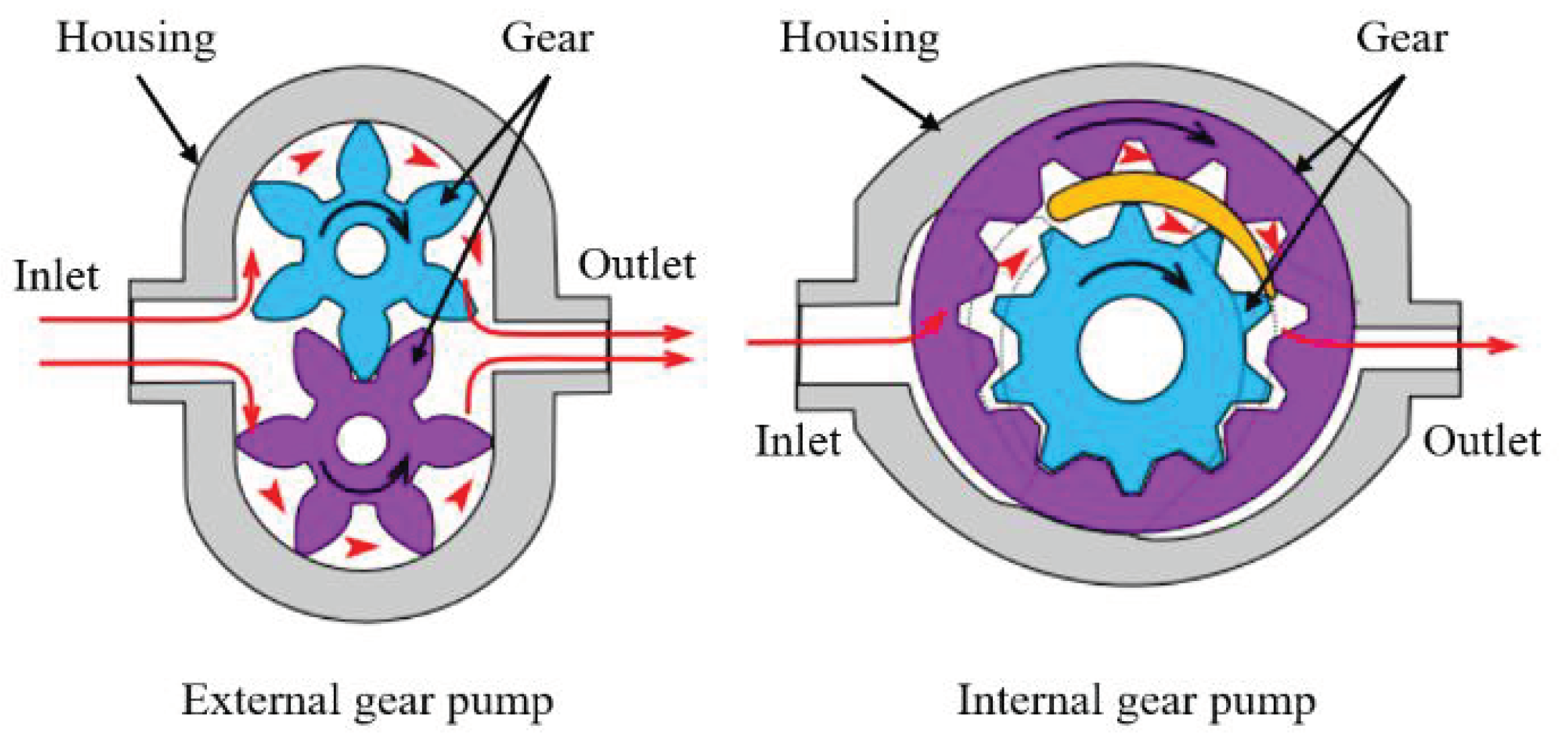
2.1. Mode of Operation of Gear Pumps

Gear pumps are quite popular for industrial purposes due to the high cost efficiency and high performance they are associated with. Being a type of positive displacement pump, it exports fluids by iteratively enclosing fixed amount of fluid using interlocking gears/clogs and transferring them mechanically via a cyclic pumping action. The fluid flow efficiencies depend significantly on the gear speed and lubrication. Essentially, there are two types of gear pumps—external and internal gear pumps, whereby the external gear pump consists of two identical, interlocking mobile gears—driver and driven supported by separate shafts while the internal gear pump operates on the same principle, but the two interlocking gears are of different sizes with one rotating inside the other. Figure 1 shows an illustration of the two types of gear pumps and their modes of operation.

As Figure 1 shows, a typical external gear pump’s mode of operation is initiated by the driver (powered by an electric motor), which meshes with the driven to create an alternating rotational motion. As the gears come out of mesh on the inlet side of the pump, they create an expanded volume, which allows liquid to flow into the cavities and is trapped by the gear teeth as the gears continue to rotate against the pump casing. This trapped fluid is transferred from the inlet, to the discharge, around the casing. As the teeth of the gears become interlocked on the discharge side of the pump, the volume is reduced and the fluid is forced out under pressure [23].

Ideally, the fluid, in addition to being pumped, serves as a lubricant for the gears to avoid wear and heat generation. In real applications, tooth wear may likely occur due to contamination or other factors like misalignment, poor design, etc. Such wear usually have impeding effects on pumping efficiency, and if not monitored, may result in total pump breakdown.

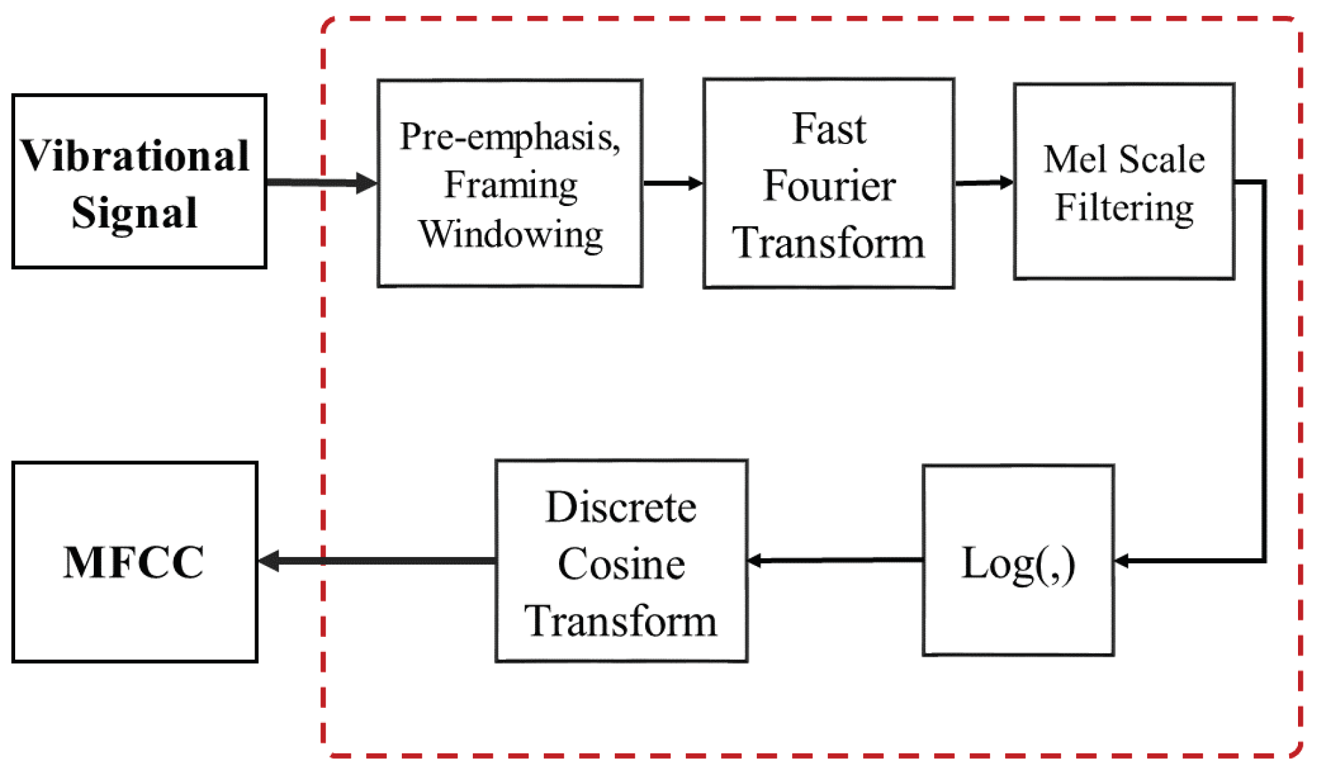
2.2. MFCC Feature Extraction

On one hand, vibration signals are often non-stationary, which often makes it uneasy to identify and isolate the low energy level fault signals. On the other hand, early wear in rotating components require sensitive signal processing techniques like MFCC for reliable wear detection efficiencies. Figure 2 shows the schematic procedure for extracting MFCCs from a signal; however, the stages summarized below provide the processes for their extraction [20].

Stage 1: Pre-emphasis, framing and windowing step provides the room for computing the fast Fourier transform (FFT) of each of the frames using Equation (1).

$$\overrightarrow{\mathrm{S}}\left(K\right)=\frac{1}{N}\sum _{i=0}^{N-1}\overrightarrow{\mathrm{A}}\left(t\right)h\left(i\right)e^{-j\left(\frac{2\pi ik}{N}\right)},0\le i\le N$$

(1)

where $\overrightarrow{\mathrm{A}}\left(t\right)$ and $\overrightarrow{\mathrm{S}}\left(k\right)$ are the input time-domain signal and the frequency-domain output of the signal, respectively, and k is the length of the FFT. N is the number of frames of the signal and $h\left(i\right)$ is the Hamming window whose value depends on a normalization factor ($\beta$).

Stage 2: Convert the frequencies from $Hz$ scale to $Mel$ scale by Mel Warping, obtain the energy spectrum and use $Mel$ band filters $(m=1,2,\dots ,M)$ spaced uniformly on the $Mel$ scale. Then, compute the log energy of each filter bank using Equation (2)

$$\overrightarrow{\mathrm{S}}\left(m\right)=ln\left(\sum _{m=0}^{N-1}{\left|\overrightarrow{\mathrm{S}}\left(k\right)\right|}^2{H}_m\left(k\right)\right),0\le m\le M$$

(2)

where $H_m$ is the transfer function of the m-th filter.

Stage 4: Finally, convert the logarithmic Mel spectrum back to the time-domain by taking the discrete cosine transform (DCT) of the spectrum using Equation (3) to extract the $Mel$ cepstral coefficients.

$$c\left(n\right)=\sum _{m=0}^{M-1}\frac{\overrightarrow{\mathrm{S}}\left(m\right)cos\pi \theta (m+0.5)}{\mathrm{\Theta }}$$

(3)

where $\theta$ is the number of frames, and $\mathrm{\Theta }$ is the number of MFCCs extracted from n^th frame of the signal ($0\le \theta \le \mathrm{\Theta }$).

In practice, the lower order MFCCs (usually 2nd–13th MFCCs) contain more discriminative spectral information from the signal.

2.3. Review of ML Algorithms for FDI

Arguably, recent advances in AI-based diagnostics methods are skewed towards the deep learning-based methods, which require no domain knowledge and/or signal processing for feature extraction [24]. Although these methods are quite impressive as recorded in many studies/applications, the expensive computational costs and magical defiance from fundamental engineering paradigms render them somewhat unreliable for cost-aware industrial applications including the case study presented herein [16].

On the bright side, traditional ML algorithms still retain their robustness and comparatively better cost efficiencies for FDI and are not limited by few data [16,17]. These algorithms, although unique in their individual architectures rely significantly on the discriminative nature of input variables for FDI; hence, the need for discriminative feature extraction from raw signals. More so, since even with discriminative features available for use, paramaterization also plays a significant role in their efficiencies [24]. These factors have motivated this study in which our objective is to explore the efficiencies of the ML algorithms for vibration-based wear detection following a MFCC-based feature extraction. It would be futile to critically discuss all the ML-based classifiers in this study; however, the subsections below provide the theoretical background of the most popular ML algorithms for diagnostics/wear detection.

2.3.1. Decision Tree

DT is one of the most cost-efficient and reliable ML algorithms and this success is attributed to its tree-based architecture. As Figure 3 illustrates, DT is an algorithm built upon a tree-like structure of decision-making rules, which functions to classify the input data into several subsets and perform predictions based on this classification [25]. A key parameter for the DT is to set proper classification variables and classification thresholds for the node(s) of each layer of the tree structure. The values for the higher nodes’ classification variables and thresholds determine the homogeneity and heterogeneity among the nodes in the lower layers [26].

In the case that the target variable is discrete, characteristic values such as the p-value of the chi-square statistic, Gini coefficient, and entropy index can be used for the classification thresholds in DT. In the case of a continuous target variable, the F-value in the analysis of variance (ANOVA) or variance reduction is used for the threshold [25]. Unlike other algorithms, DT is a typical white-box model and it does not hide what is used as the threshold for each node’s classification. It also works for both numerical and categorical data and has a simple formula, and thus can process massive data in a relatively short time. However, the pruning process for avoiding the over-fitting and under-fitting problems in DT should be based on experience and, even in the cases of having proper values for pruning, the complete resolution of these problems is not guaranteed [25,26].

2.3.2. Random Forest

RF is an algorithm designed to overcome the limitation of DTs by deploying multiple decision trees simultaneously [27]. As Figure 4 shows, RF lets the input samples pass through multiple tree structures with different classification criteria and stores the outcomes from each tree. It compares these different outcomes to single out the most common one as the final result of the classification.

By changing its key parameter namely the number of trees, RF can minimize the over-fitting problem—the biggest weakness of DT [27].

2.3.3. k-Nearest Neighbor

KNN is a machine learning algorithm that performs classification based on the assumption that a set of data with a similar feature would also have similar feature values [28]. For instance, consider the two types of data represented by green squares (GS) and yellow triangles (YT) in Figure 5, a circle drawn around the data—red star (RS) suggests it can be classified as a YT since there are more YTs than GSs inside the circle. However, if the circle expands to the area bounded by the broken line as the value for k parameter, indicating a distance in Euclidean space changes, there would be three GSs and two YTs in the circle so that RS would be reclassified as GS.

This way of classification could work well for evenly distributed data sets; however, in the case that the data has only small differences between them, its classification accuracy could significantly decrease. Furthermore, even a little change in the k-value could have a huge influence on its accuracy [28]. Therefore, to make the data set evenly reflect all the feature values under consideration, the normalization of data is required. For the normalization, the data could be converted into a fixed value between 0 and 1; the average value or standard deviation could also be used.

2.3.4. Naïve Bayes Classifier

NBC is a type of supervised learning classification algorithms based on Bayes’ theorem, which defines the relationships between two conditional probabilities about a certain event by using the information provided in advance about the event [29]. The theorem can be described in Equation (1) below.

$$P(A\mid B)=\frac{P(A\cap B)}{P\left(B\right)}=\frac{P(A\mid B)·P\left(A\right)}{P\left(B\right)}$$

(4)

where $P\left(A\right)$ and $P\left(B\right)$ are the prior probability of the event A and that of the event B, respectively, whereas $P(A\mid B)$ and $P(B\mid A)$ indicate the prior probability of A in the condition that B has already happened and that of B in the condition that A has already happened, respectively.

There are multiple classification models based on Bayes’ theorem, such as Gaussian Naïve Bayes, Bernoulli Naïve Bayes, and Multinomial Naïve Bayes. Compared to other supervised machine learning algorithms, Naïve Bayes Classification has a relatively simple model with simple computational procedures, but also has a superior classification capability. By assuming each probability as a separable condition, it can alleviate the problem that could be caused by multiple dimensions [30].

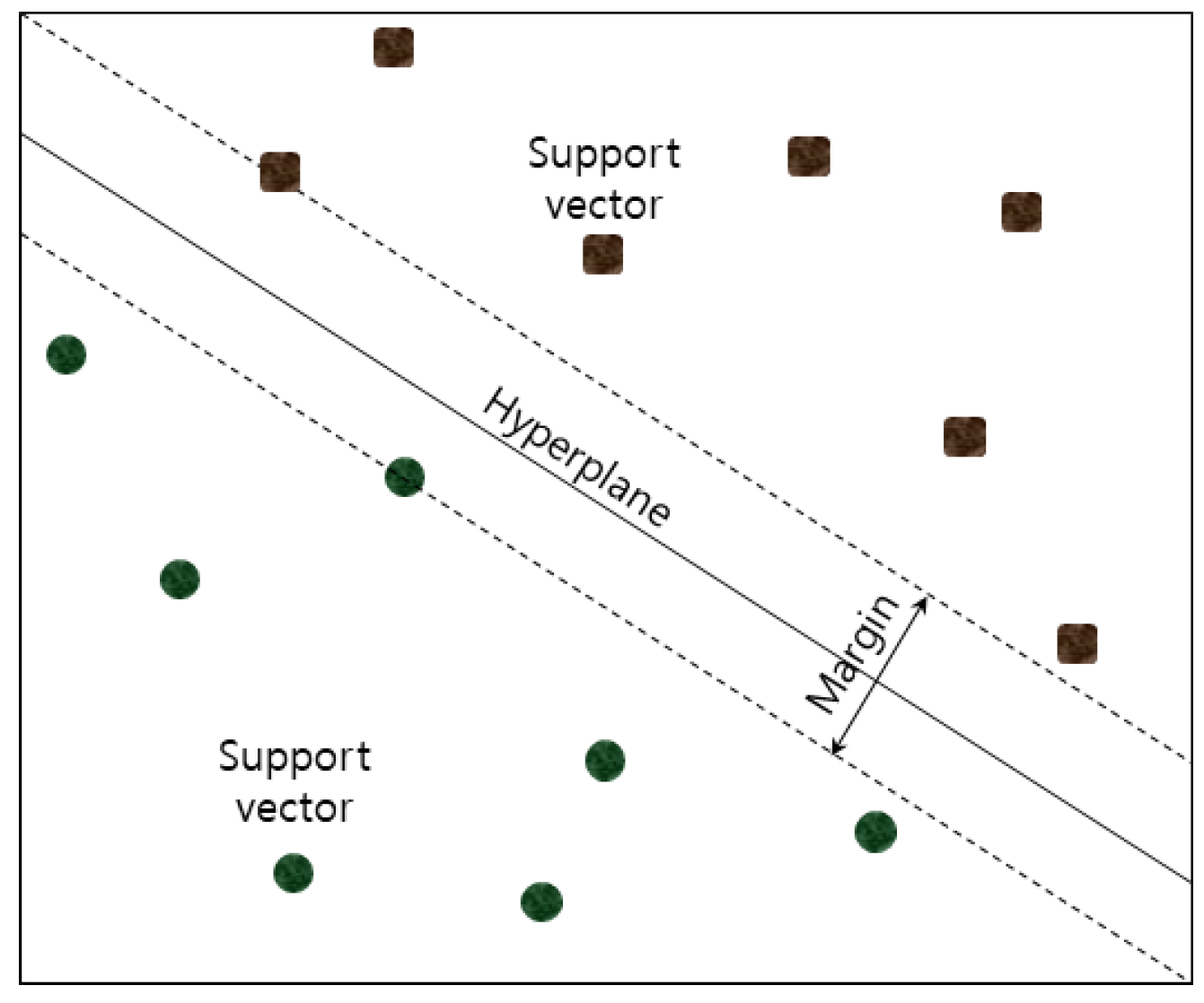
2.3.5. Support Vector Machines

The SVM is an algorithm that creates a decision boundary between data classes by creating a hyper-plane for separation using the support vectors. It allows users to set the gamma parameter of decision boundary—the distance which the samples in either side can exchange influences to each other, the C (regularisation) parameter, and various kernels—linear, polynomial, radial-basis function (RBF), etc. [20]. As Figure 6 illustrates, the optimal decision boundary drawn among the data types A (brown squares) and B (green circles) should be what divides them into two distinguishable parts without being overlapped with both classes. The regularisation parameter determines the distance between the decision boundary and separation, and could be adjusted based on experience.

By default, SVMs have a high computation speed for binary cases, as it calculates only the distances of nearby data for drawing a decision boundary between the classes; however, as its parameter values increase, the inherent complexity and computational costs also increases. By setting proper parameters, the user therefore can perform the classification even with the data set with an ambiguous boundary [20].

2.3.6. Multi-Layer Perceptron

The MLP is a traditional feed-forward neural network (FFNN), which typically consists of three basic structures: an input layer, a hidden layer, and an output layer [31]. Due to its architecture and learning rule, it is quite efficient for supervised and unsupervised cases, and are particularly efficient for classifications problems. A typical MLP with three (3) hidden layers (to form a deep neural network) is illustrated in Figure 7 where the layers comprise of several nodes (m nodes in the input layer, p, q, and r nodes in the first, second, and third hidden layers respectively, and n nodes in the output layer).

Each node exports its input value to the next layer via a weighted forward propagation process such that the input to the output layer (for instance)—$O_{i_{-}}in$ received by node $O_i$ is the sum of the activated outputs of layer $h_3$ multiplied by the corresponding connection weight matrix $w_4$ using Equation (5).

$$O_{i_{-}in}=\sum _{i=1}^r{w}_4\ast A\left[i\right]$$

(5)

where $A\left[i\right]$ is the activated outputs of the nodes in $h_3$.

The output $O_{i_{-}out}$ from each of the output nodes $O_i$ is obtained by passing the inner product $O_{i_{-}in}$ through a nonlinear activation function f using Equation (6):

$$O_{i_{-}out}=f\left(O_{i_{-}in}\right)$$

(6)

where the choice of f ranges across Sigmoid, Tanh, rectified linear unit (ReLU), Leaky ReLU, etc. The automatic (supervised) learning process of MLPs by gradient descent enables for minimizing the squared error in the predicted outputs via a back-propagation of weights using Equation (7):

$$E={\left(y-O_{i_{-}out}\right)}^2$$

(7)

where E is the prediction error (cost function) and y is the desired output label.

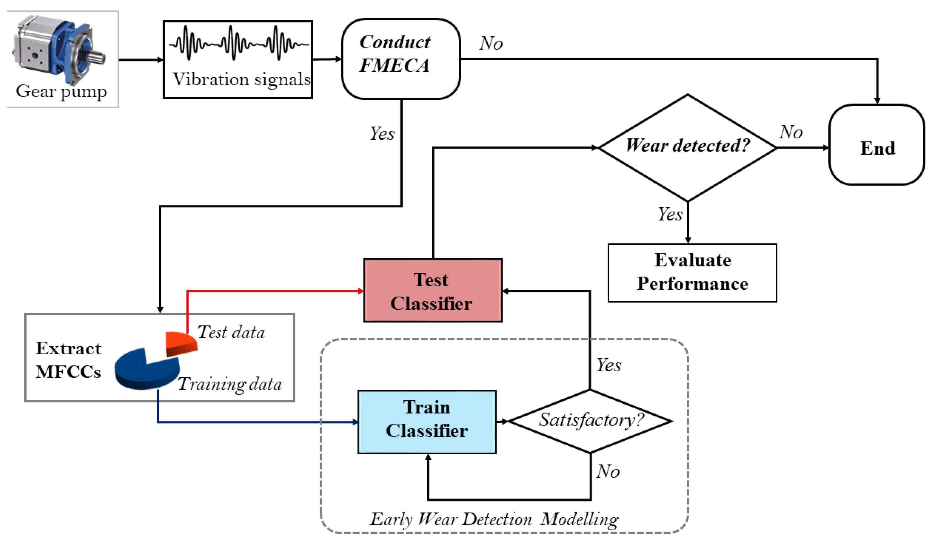
3. Proposed Wear Detection Model

In this section, an overview of the FMECA and the proposed wear detection model for gear pumps is presented. Figure 8 presents the proposed model’s flowchart.

As shown, a FMECA analysis is optionally conducted, after which vibration signals are collected via an accelerometer for use by the wear detection model. The subsections below explain, in detail, the different modules in the proposed model.

3.1. FMECA

Over the years, there has been a dominant propensity of managers and engineers to reduce the risk/failure in products—system, design, process, and/or service, and these have motivated the growth of reliability engineering, not only to reduce the risk, but also to define those risks whenever possible [3]. Among many methods including statistical, analytical, and visual methods, FMECA—a modification of the traditional FMEA is a tool which offers a less mathematical (but highly reliable) methodology for evaluating a system, design, process, or service to discover possible ways that failures (problems, errors, risks, concerns) can occur, as well as their level(s) of severity and/or criticality [3,4].

As motivated by the US military to change from an approach of find failure and fix it to anticipate failure and prevent it in the late 1940s, FMECA has also become a valuable tool in industries and functions by calculating a criticality and ranking the failure modes on a criticality matrix. Prior to performing the full FMECA, the traditional FMEA is performed to evaluate the risk priority number (RPN), which is the product of rankings for the severity (Sr), the likelihood of failure (Fr), and detectability (Dr) of the failure. Fundamentally, the Sr, Fr, and Dr values for each failure mode ranges between 1 (least-ranking) and 10 (highest ranking) failure modes, respectively. From the criticality matrix, FMECA results can be ranked based on the RPN. Other FMECA levels may be employed depending on the product, design, and service specific levels.

In reality, while addressing severity is key to understand the risk of a particular failure mode, that does not mean that the risk of the failure mode is high because, while severity may be high, if the severity and/or failure likelihood of this failure is low or if the detection methods are efficient, the overall risk (computed by RPN) may be low and the failure may not be a priority. Hence, a high priority level of a failure mode depends on a high Sr, FR, and Dr, while the reverse is the case for a low priority failure mode [3,4].

3.2. MFCC Feature Extraction

Following a FMECA on the pump as an optional activity, the wear detection model accepts the highly non-stationary vibration signals and extracts useful MFCCs (MFCC2 – MFCC13), which form the fault features for use by the ML-based classifiers for diagnosis. The feature extraction module offers a high discriminative fault feature extraction performance on one hand and a computational cost efficiency on the other hand as verified in [18]. The feature extraction process is simultaneously done for the training data-set and test data-set for training and testing the model’s efficiency, respectively.

3.3. ML-Based Modelling and Wear Detection

Inspired by different learning rules as discussed in the previous section, ML-based classifiers receive the training data-set (labelled MFCC feature set) for dynamic modelling in a supervised manner. Following a satisfactory training (minimum binary cross-entropy loss) via an exhaustive grid search for each model’s optimal parameters, the model(s) is(are) deployed on the test data for testing (wear detection). Specifically, the binary cross-entropy is a loss function that is used in binary classification tasks just as presented in the proposed study’s problem set—wear detection.

After a successful training of the model(s), the test data-set is employed for an unsupervised testing process whereby the test data-set contains unlabelled MFCC features extracted from vibration samples from the gear pump at healthy and casing wear conditions, respectively. By so doing, the model either detects whether wear has occurred in the gear casing or not given a set of input features.

3.4. Performance Evaluation

The wear detection performance of the model is evaluated using standard binary classification metrics—accuracy, precision, F1-score, recall, confusion matrix, and a visualization assessment. The visualization assessment provides the avenue to visually assess and control the wear detection performance of each model by observing the separation planes generated by the ML models.

4. Experimental Study and Analysis

This section presents a case study whereby a MFCC-based fault diagnosis of AP3.5/100 external gear pump manufactured by BESCO is explored.

4.1. FMECA of Gear Pump

As a condition for the abrasion test, an in-depth study on the common failure modes which gear pumps are prone to is crucial. FMECA offers a paradigm for understanding the most common failure modes. This provides the conviction for compelling the pump to be operated under certain failure conditions (s) for the proposed study. To achieve this, this study decomposes its structure into the eight most critical component parts—the gear case, cover, drive shaft gear, follower shaft gear, shroud, seal, bearing, and fastening bolt.

Table 1. FMECA results on AP3.5/100 external gear pump manufactured by BESCO.

Component	Function	Failure Mode	Cause	Effect	Criticality
					Sr	Dr	Fr	RPN
Gear Case	Structure flow distribution	wear	Contaminants, fatigue	Outside leakage, efficiency reduction	5	2	2	20
		Transient Resistance	fluid passage Narrow	Noise	3	2	1	6
Cover	Structure	wear	Uneven load	Outside leakage, efficiency reduction	9	3	3	81
		Corrosion	Moisture, surface contamination	Outside leakage	5	3	1	15
Drive shaft gear	Power transmission	Gear hit damage	Foreign substance, fatigue	Vibration and noise	7	2	3	42
		Gear end wear	Contaminants, fatigue	Outside leakage, efficiency reduction	7	3	2	42
		Damage	Increased fatigue, stress concentration	Inoperable	5	3	1	15
Follower shaft gear	fluid suction, discharge	Gear hit damage	Foreign substance, fatigue	Vibration and noise	7	2	3	42
		Gear end wear	Contaminants, fatigue	outside leakage, efficiency reduction	7	3	2	42
		Damage	Increased fatigue, stress concentration	Inoperable	5	3	1	15
Shroud	Vibration damping	wear	Uneven load	Leakage, efficiency reduction	7	3	2	42
		Vibration	Design failure	Vibration and noise	5	3	1	15
Seal	fluid leak prevention	Damage	Aging, cracking	Internal/external leakage	7	3	2	42
Bearing	Rotation and support	wear	Foreign substance	Vibration, efficiency reduction	7	3	2	42
		Crack	Fatigue	Friction and vibration	5	3	1	15
Fastening bolt	Housing fastening	Loosening	Poor assembly	Internal/external leakage	7	3	2	42
		Damage	Increased fatigue, stress concentration	Outside leakage	5	3	1	15

presents the possible failure modes and their Sr, Fr, Dr and RPN values for each component’s failure modes.

From the FMECA results above, the most critical failure mode is the housing wear (with a RPN of 81 constituted by high Fr, Sr, and Dr values in Table 1), which are commonly caused by uneven load distribution. In the abrasion test designed to replicate this condition, the vibrations caused by the Fe${}_2$O${}_3$ particles were collected for the wear detection process [4,23].

4.2. Gear Pump Abrasion Test

The proposed experimental setup shown in Figure 9 was performed at room temperature and standard humidity level as suggested by the KS A 0006 environmental standards for tests [32]. The working fluid was mixed with Fe${}_2$O${}_3$ particles and the pump powered by a 1750 RPM electric motor to generate a delivery pressure of about 100 bar [23,33,34].

The setup for the test consists of the following components as shown in Figure 9—a reservoir for the working fluid, gear pump for the test, a 3-phase induction motor (rated 220 V, 0.75 KW, 60 Hz, 1720 rpm) for driving the gear, a relief valve that controls the fluid flow to produce certain fluid pressure, a flow meter to measure the amount of fluid flow, a hydraulic meter to measure the pressure, vibration sensor/accelerometer for data collection, a 12V DC adapter for powering the national instruments data acquisition (NI DAQ), and NI 9234 module to acquire vibration signals which are then digitally saved in “.csv” files in a computer using LabView software [23]. As the motor is turned on, the gear pump begins to work and sucks the fluid from the reservoir, and then compresses it and discharges through the outlet back to the reservoir. As the discharged fluid flows through the flow meter and the relief valve, high pressure is generated.

4.3. Abrasion Test Results

Ideally, a small space (with minimal contact) between the housing and rotating gears ensures that fluid is constantly forced out under pressure. Hence, pumping efficiency is ensured by the lubricating action of the working fluid between the gears and the pump housing. Unfortunately, in the event of fluid contamination, the pump’s housing may experience wear, which may worsen over time and reduce pumping efficiency if not properly monitored. The abrasion test was stopped when the output pressure dropped to the minimum pressure of 50 bar required to operate the pump. During this period, there wasn’t any significant level of noise generated by the pump to indicate some level of fault in the pump. This would have been the tell-tale sign of failure, but often an early wear occurrence does not produce distinguishable noise/vibration levels. Figure 10 shows the pictorial view of the gear pump housing highlighting the contact area between the gears and the housing (refer to Figure 10a) whereby Figure 10b,c are zoomed views of the highlighted area after clean working fluid was used and after the abrasion test, respectively, while Figure 10d,e are their respective surface profiles for Figure 10b,c respectively.

As Figure 10b shows, after the test, the contact surface area between the housing and the gear turned out to be worn significantly in comparison to the new/healthy contact surface before the test (see Figure 10a). This is as a result of the increased friction between the gears and the housing due to the wear effects from the Fe${}_2$O${}_3$ particles. A closer observation of the pump’s housing surface profile in Figure 10e reveals the surface wear intensity by the high frequency components (in red). This is in clear contrast to the little/negligible wear represented by lower frequencies (in blue) in the same contact surface area when clean working fluid was used (refer to Figure 10d).

4.4. Feature Engineering

The raw vibration signals generated from the abrasion test were too ambiguous for direct use for diagnosis, so they were cleaned, pre-processed and MFCC feature extraction initiated. Figure 11 presents a portion of the whole data gathered from the accelerometer during the abrasion test. It shows that the amplitudes of the vibration data had gradually increased earlier but, after the abrasion reached a certain level, they began to increase rapidly.

MFCCs are quite sensitive to transient and spectral changes in vibration signals [18,21]; hence befitting for early wear detection. The useful MFCCs (MFCC2–MFCC13) have shown to be very effective for low-frequency feature extraction and are suitable for the proposed case study. Accordingly, 13 MFCC features were extracted, respectively, from the training and test datasets. Invariably, the salience of these features for wear detection lies in their discriminance. To assess the discriminance of extracted MFCC features, a correlation test was performed on the features using the Spearman’s correlation test [35]. The results are presented in Figure 12.

As shown in Figure 12, the significantly low correlation values between the features insinuates a high discriminance between them—a necessary feature characteristic which ensures accurate classification performance/diagnosis by the classifier(s) [23]. With the highest correlation existing only between MFCC 6 and MFCC 7 with a 0.68 correlation value while the rest have really low correlation values, it can be deduced that the features are highly discriminant and suitable for diagnostics.

4.5. ML-Based Wear Detection

The learning-based classifiers listed in

Table 2. Optimal parameters for classifiers.

Algorithm	Parameter	Value
Logistic regression (LR)	regularisation	L1
KNN	k	5
Linear SVM (SVM-Lin)	kernel	Linear
Gaussian-kernel SVM (SVM–RBF)	C, gamma	10, 1
Gradient boosting Classifier (GBC)	n estimators	1000
DT	Pruning	12
RF	n estimators	120
Multi-layer perceptron (MLP) classifier	n layers, learning rate	3, 0.001
NBC	Gaussian	–
Adaboost classifier (ABC)	n estimators, learning rate	50, 0.1
Quadratic discriminant analysis (QDA)	regularization	0.001
Gaussian process classifier (GPC)	kernel	RBF

were employed on the training dataset, respectively, in a supervised manner and also tested on the test dataset in an unsupervised manner after training.

As Table 2 shows, each algorithm has its unique parameters and architecture; hence, requires domain experience for optimum efficiency. Over several iterations and repeated trials, the most optimal parameters for each algorithm were discovered following an exhaustive parameter tuning process, which were then recorded in Table 2. Following a 10-fold cross validation of each algorithm on the test data, Figure 13 shows the confusion matrix of the respective predictions made by the classifiers.

Overall, the models were quite effective; however, a closer look at Figure 13 reveals that the SVM and SVM-RBF models, respectively, returned the least false positives (FP) $1.7\%$; however, the models’ limitations are observed in the $19.4\%$ false negative (FN) predictions. This obviously returns $98.3\%$ true positive (TP) and $80.6\%$ true negative (TN) from both models (see Figure 13c,d). In contrast, although with a high FP of $5.3\%$, the RF returns a FN of $4.7\%$, which invariably returns the highest prediction performances—TP and TN of $94.7\%$ and $95.3\%$, respectively.

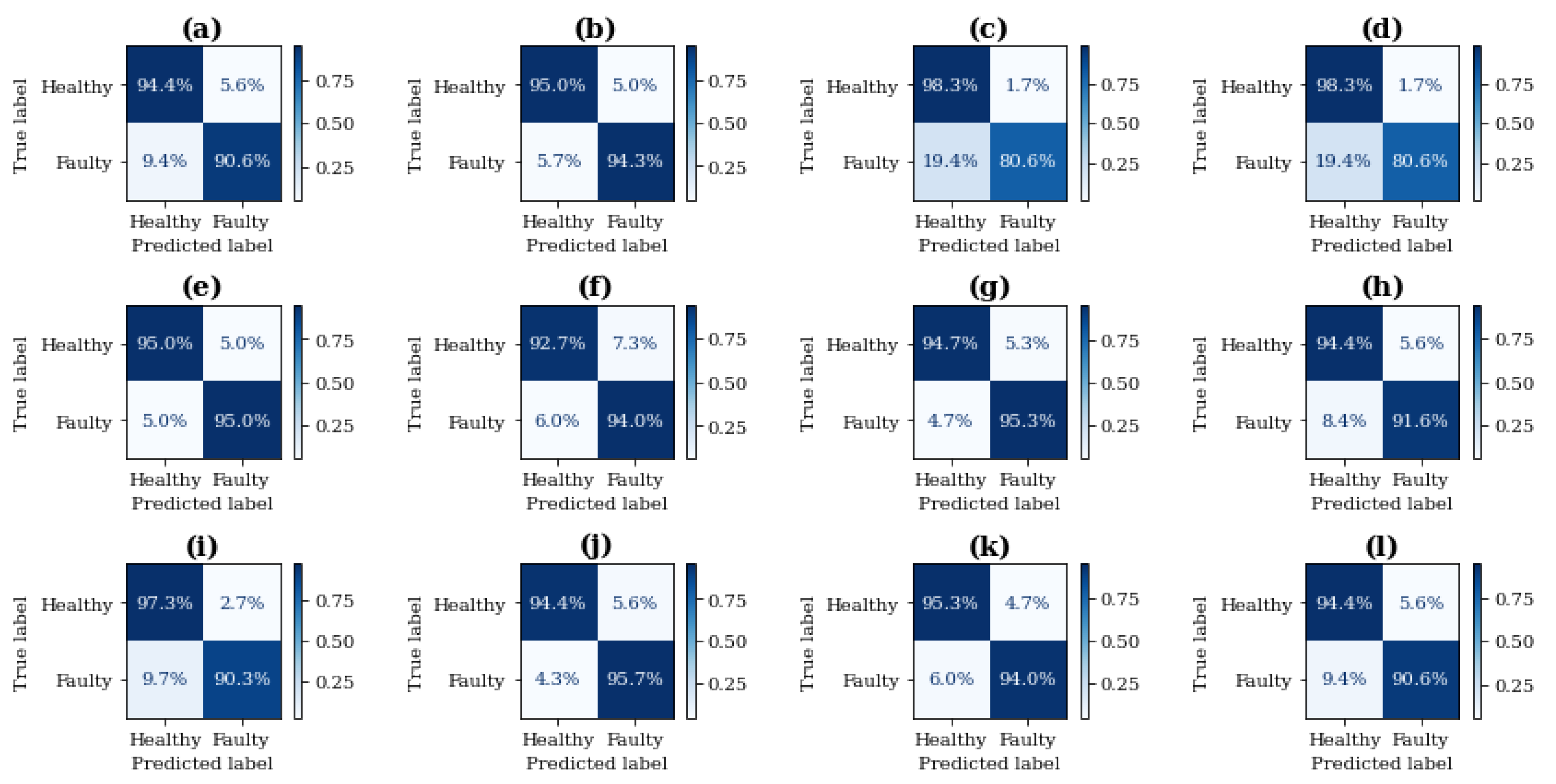
4.6. Performance Evaluations

Individually, it may be hectic to draw a global conclusion based on the confusion matrix comparison since it provides a class-based (local) evaluation of a model; therefore, global evaluation metrics like the accuracy, precision, recall, F-1 score, and training computational costs (in seconds) were employed for a more comprehensive comparative analysis of the algorithms [22].

Table 3. Global performance comparison of ML models.

Algorithm	Accuracy (%)	Precision (%)	Recall (%)	F1-Score (%)	Cost (Secs)
LR	92.50	92.56	92.49	92.50	0.03697
k-NN	94.67	94.67	94.67	94.67	0.01035
SVM-Lin	89.50	90.79	89.47	89.41	0.14247
SVM–RBF	89.50	90.79	89.47	89.41	9.35574
GBC	94.83	94.83	94.83	94.83	12.84497
DT	93.00	93.00	93.00	93.00	0.01374
RF	95.17	95.17	95.17	95.17	17.61929
MLP	93.33	93.34	93.33	93.33	15.47579
NBC	93.83	94.06	93.82	93.82	0.0800
ABC	95.00	95.01	95.00	95.00	0.94587
QDA	94.67	94.68	94.66	94.67	0.0740
GPC	92.50	92.56	92.49	92.50	6.52012

summarises the performance of the classifiers based on these metrics. Accuracy globally evaluates a model’s predictive capability to make correct class predictions, precision returns the percentage of the classes that are true among those the model predicts correctly as true, recall measures the percentage of the cases that the model predicts as true among all of those that are really true, while the F-1 score is the harmonic average of precision and recall.

As observed from Table 3, the RF is the most accurate with accuracy, precision, recall, and F1-score of $95.17\%$, respectively. Although the most accurate, it is the most computationally expensive amongst the algorithms with about $17.62$ s computational time. This is followed by the ABC with $95\%$ accuracy with a much lesser computational time of approximately 1 s. Overall, the RF, SVM–RBF, GBC, GPC, and MLP are the most computationally expensive (based on the test data) while the fast algorithms like the DT and k-NN show quite impressive computational speeds of approximately 0.01 s, respectively. This comparison hints at providing a paradigm for choice of classifier depending on the metric of interest. As is observed in most real-life situations, computational speed is mostly always highly considered, but not to the detriment of predictive efficiencies. In such a situation, one may opt for the ABC considering that although it is not the most accurate, the low computational costs it is associated with renders it more reliable than the others, while the RF would be considered in situations where computational resources are abundant or accuracy is of utmost importance.

4.7. Fault Visualization

Most often, visualizations play an important role for assessing the predictive efficiencies of a diagnostic model; however, in cases where the number of features exceed pictorially presentable dimensions (a maximum of three dimensions), it is advised to employ dimensionality reduction algorithms to reduce the feature dimension for visualization. Several dimensionality reduction algorithms abound for exploration; however, the authors prefer the locally linear embedding (LLE) algorithm over the popular principal component analysis (PCA) and its variants due to the LLE’s comparative superiority for preserving data’s local structure in the newly reconstructed/reduced feature space. Figure 14 shows the fault isolation visualizations of the classifiers on the two-dimensional LLE features from the 13-dimensional MFCC feature vector.

The data points in blue and red circles represent the LLE samples for healthy and faulty states of the gear pump. As shown by the grids, each of the algorithms are quite effective for creating a distinctive hyper-plane between both operating conditions; hence, they are suitable for early wear detection.

5. Conclusions and Drawn Insights

Development (and improvement) of fault detection and isolation modules have become a major interest for researchers, academic institutions, and industries in view of more accurate prognostics and health management. State-of-the-art cost-aware methods are centred on the use of signal processing tools for feature extraction integrated with machine learning algorithms, which provide high accuracy probability for fault isolation with minimal false alarm rates.

Addressing severity of failure modes under FMECA is key to understanding the risk of the failure modes; however, also assessing the likelihood of failure, severity level, and detection rate provides a more reliable perspective for prioritizing failure modes. Following a FMECA on the proposed case study—an AP3.5/100 external gear pump manufactured by BESCO, the study designed an experimental replication of the housing abrasion caused by the inflow of foreign particles into the gear pump to collect vibration data at normal state and failure states. The result of gear pump FMECA identified the fluid leakage and vibrations resulted from the foreign particle-caused abrasion as the most severe, critical and highly probable failure mode. On the other hand, MFCC features were extracted from vibration signals for proper characterization of the pump for early wear detection using traditional machine learning methods with empirical assessments supporting their discriminance levels—a major feature evaluation factor for diagnostics. The accuracies of the machine learning algorithms were explored with the random forest emerging the most accurate with 95.17% test accuracy, precision, recall, and F1-score, respectively. Unfortunately, the results also reveal that it is the most computationally expensive; hence is recommended for applications where computational resource isn’t a major factor. Although not the most accurate, the adaboost classifier’s low computational costs makes it more reliable for cost-aware applications.

Ideally, failure diagnostics precede a prognostics scheme whereby future wear/degradation of the target component are estimated using regression and/or forecasting tools for remaining useful life prediction. Considering that the proposed study reveals that casing wear is the most severe and critical failure mode, we believe that a prognostics scheme should prioritize casing wear/degradation, since it is the most highly probable, severe, and critical failure mode. As continued research, we intend to replicate a run-to-failure experiment in this failure mode for developing a befitting prognostics scheme/model for wear/degradation monitoring and remaining useful estimation.

References

1. Ciani, L.; Guidi, G.; Patrizi, G.; Galar, D. Condition-Based Maintenance of HVAC on a High-Speed Train for Fault Detection. Electronics 2021, 10, 1418. [Google Scholar] [CrossRef]
2. Casoli, P.; Pastori, M.; Scolari, F.; Rundo, M. A Vibration Signal-Based Method for Fault Identification and Classification in Hydraulic Axial Piston Pumps. Energies 2019, 12, 953. [Google Scholar] [CrossRef] [Green Version]
3. Stamatis, D.H. Failure Mode and Effect Analysis FMEA from Theory to Execution, 2nd ed.; ASQ Quality Press: Milwaukee, WI, USA, 2003. [Google Scholar]
4. MIL-STD-1629A, Military Standard: Procedures for Performing a Failure mode, Effects, and Criticality Analysis (24 NOV 1980). Available online: https://extapps.ksc.nasa.gov/Reliability/Documents/milstd1629_FMEA.pdf (accessed on 13 January 2021).
5. Gu, Y.; Li, W.; Zhang, J.; Qiu, G. Effects of Wear, Backlash, and Bearing Clearance on Dynamic Characteristics of a Spur Gear System. IEEE Access 2019, 7, 117639–117651. [Google Scholar] [CrossRef]
6. Natili, F.; Daga, A.P.; Castellani, F.; Garibaldi, L. Multi-Scale Wind Turbine Bearings Supervision Techniques Using Industrial SCADA and Vibration Data. Appl. Sci. 2021, 11, 6785. [Google Scholar] [CrossRef]
7. Dineva, A.; Mosavi, A.; Gyimesi, M.; Vajda, I.; Nabipour, N.; Rabczuk, T. Fault Diagnosis of Rotating Electrical Machines Using Multi-Label Classification. Appl. Sci. 2019, 9, 5086. [Google Scholar] [CrossRef] [Green Version]
8. Esakimuthu Pandarakone, S.; Mizuno, Y.; Nakamura, H. A Comparative Study between Machine Learning Algorithm and Artificial Intelligence Neural Network in Detecting Minor Bearing Fault of Induction Motors. Energies 2019, 12, 2105. [Google Scholar] [CrossRef] [Green Version]
9. Ju, Y.J.; Kim, M.S.; Kim, K.S.; Lee, J.H. Comparison of Machine Learning Algorithms Applied to Classification of Operating Condition of Rotating Machinery. J. Comput. Des. Eng. 2020, 5, 77–87. [Google Scholar] [CrossRef]
10. Ding, C.; Zhao, M.; Lin, J. Sparse feature extraction based on periodical convolutional sparse representation for fault detection of rotating machinery. Meas. Sci. Technol. 2021, 32, 1. [Google Scholar] [CrossRef]
11. Qiao, Z.; Elhattab, A.; Shu, X.; He, C. A second-order stochastic resonance method enhanced by fractional-order derivative for mechanical fault detection. Nonlinear Dyn. 2021, 106, 707–723. [Google Scholar] [CrossRef]
12. Qiao, Z.; Shu, X. Coupled neurons with multi-objective optimization benefit incipient fault identification of machinery. Chaos Solitons Fractals 2021, 145, 110813. [Google Scholar] [CrossRef]
13. Akpudo, U.E.; Hur, J.-W. D-dCNN: A Novel Hybrid Deep Learning-Based Tool for Vibration-Based Diagnostics. Energies 2021, 14, 5286. [Google Scholar] [CrossRef]
14. Kim, S.; Akpudo, U.E.; Hur, J.-W. A Cost-Aware DNN-Based FDI Technology for Solenoid Pumps. Electronics 2021, 10, 2323. [Google Scholar] [CrossRef]
15. Akpudo, U.E.; Hur, J.-W. A CEEMDAN-Assisted Deep Learning Model for the RUL Estimation of Solenoid Pumps. Electronics 2021, 10, 2054. [Google Scholar] [CrossRef]
16. Akpudo, U.E.; Hur, J.W. Towards bearing failure prognostics: A practical comparison between data-driven methods for industrial applications. J. Mech. Sci. Technol. 2020, 34, 4161–4172. [Google Scholar] [CrossRef]
17. Han, T.; Jiang, D.; Zhao, Q.; Wang, L.; Yin, K. Comparison of random forest, artificial neural networks and support vector machine for intelligent diagnosis of rotating machinery. Trans. Inst. Meas. Control 2017, 40, 2681–2693. [Google Scholar] [CrossRef]
18. Akpudo, U.E.; Hur, J. A Cost-Efficient MFCC-Based Fault Detection and Isolation Technology for Electromagnetic Pumps. Electronics 2021, 10, 439. [Google Scholar] [CrossRef]
19. Caesarendra, W.; Tjahjowidodo, T. A Review of Feature Extraction Methods in Vibration-Based Condition Monitoring and Its Application for Degradation Trend Estimation of Low-Speed Slew Bearing. Machines 2017, 5, 21. [Google Scholar] [CrossRef]
20. Akpudo, U.E.; Hur, J.W. A Multi-Domain Diagnostics Approach for Solenoid Pumps Based on Discriminative Features. IEEE Access 2020, 8, 175020–175034. [Google Scholar] [CrossRef]
21. Tang, S.; Zhu, Y.; Yuan, S.; Li, G. Intelligent Diagnosis towards Hydraulic Axial Piston Pump Using a Novel Integrated CNN Model. Sensors 2020, 20, 7152. [Google Scholar] [CrossRef]
22. Akpudo, U.E.; Hur, J.W. Intelligent Solenoid Pump Fault Detection based on MFCC Features, LLE and SVM. In Proceedings of the International Conference on AI in Information and Communication (ICAIIC 2020), Fukuoka, Japan, 19–21 February 2020; pp. 404–408. [Google Scholar]
23. Lee, G.H.; Shin, B.C.; Hur, J.W. Fault Classification of Gear Pumps Using SVM. J. Appl. Reliab. 2020, 20, 187–196. [Google Scholar] [CrossRef]
24. Tjoa, E.; Guan, C. A Survey on Explainable Artificial Intelligence (XAI): Toward Medical XAI. IEEE Trans. Neural Netw. Learn. Syst. 2020, 32, 4793–4813. [Google Scholar] [CrossRef] [PubMed]
25. Asman, S.H.; Ab Aziz, N.F.; Ungku Amirulddin, U.A.; Ab Kadir, M.Z.A. Decision Tree Method for Fault Causes Classification Based on RMS-DWT Analysis in 275 kV Transmission Lines Network. Appl. Sci. 2021, 11, 4031. [Google Scholar] [CrossRef]
26. Li, Z.; Zhang, Y.; Abu-Siada, A.; Chen, X.; Li, Z.; Xu, Y.; Zhang, L.; Tong, Y. Fault Diagnosis of Transformer Windings Based on Decision Tree and Fully Connected Neural Network. Energies 2021, 14, 1531. [Google Scholar] [CrossRef]
27. Xu, G.; Liu, M.; Jiang, Z.; Söffker, D.; Shen, W. Bearing Fault Diagnosis Method Based on Deep Convolutional Neural Network and Random Forest Ensemble Learning. Sensors 2019, 19, 1088. [Google Scholar] [CrossRef] [PubMed] [Green Version]
28. Yang, J.; Sun, Z.; Chen, Y. Fault Detection Using the Clustering-kNN Rule for Gas Sensor Arrays. Sensors 2016, 16, 2069. [Google Scholar] [CrossRef] [PubMed] [Green Version]
29. Pietrzak, P.; Wolkiewicz, M. On-line Detection and Classification of PMSM Stator Winding Faults Based on Stator Current Symmetrical Components Analysis and the KNN Algorithm. Electronics 2021, 10, 1786. [Google Scholar] [CrossRef]
30. Zhang, N.; Wu, L.; Yang, J.; Guan, Y. Naive Bayes Bearing Fault Diagnosis Based on Enhanced Independence of Data. Sensors 2018, 18, 463. [Google Scholar] [CrossRef] [Green Version]
31. Oh, S.H. Improving the Water Level Prediction of Multi-Layer Perceptron with a Modified Error Function. Int. J. Contents 2018, 13, 23–28. [Google Scholar] [CrossRef]
32. KS A 0006:2001. Standard Atmospheric Conditions for Testing. Korean Agency for Technology and Standard, Eumseong-gun, Korea. 2014, pp. 1–2. Available online: https://infostore.saiglobal.com/en-us/standards/ks-a-0006-2001-639645_saig_ksa_ksa_1524462/ (accessed on 13 January 2021).
33. Pumps, Hydraulic, Variable Flow. In General Specification for MIL-P-19692 E; Department of Defense: Washington, DC, USA, 1994; pp. 20–21, 24–25. Available online: http://everyspec.com/MIL-SPECS/MIL-SPECS-MIL-P/MIL-P-19692E_38833/ (accessed on 13 October 2020).
34. Test Powders and Test Particles; KS A 0090, Korean Agency for Technology and Standards: Eumseong-gun, Korea, 2017. Available online: https://shop.standards.ie/Store/Details.aspx?ProductID=2036387 (accessed on 13 October 2020).
35. Nasir, I.M.; Khan, M.A.; Yasmin, M.; Shah, J.H.; Gabryel, M.; Scherer, R.; Damaševičius, R. Pearson Correlation-Based Feature Selection for Document Classification Using Balanced Training. Sensors 2020, 20, 6793. [Google Scholar] [CrossRef]
Figure 1. Operating mode of gear pump (from [23]).
Electronics 10 02939 g001
Figure 2. MFCC feature extraction processes.
Electronics 10 02939 g002
Figure 3. Illustration of a typical DT architecture.
Electronics 10 02939 g003
Figure 4. Illustration of a typical RF architecture.
Electronics 10 02939 g004
Figure 5. Illustration of a typical KNN architecture.
Electronics 10 02939 g005
Figure 6. Illustration of a typical SVM architecture.
Electronics 10 02939 g006
Figure 7. A DNN with three hidden layers (MLPs).
Electronics 10 02939 g007
Figure 8. Proposed wear detection model.
Electronics 10 02939 g008
Figure 9. Diagram showing the experimental setup and and data collection process.
Electronics 10 02939 g009
Figure 10. Images of the housing (a) showing the contact area between the gears and the housing, (b) the contact area with clean working fluid (c) the contact area after the abrasion test, (d) surface profile for contact area with clean working fluid, and (e) surface profile for contact area after abrasion test.
Electronics 10 02939 g010
Figure 11. Gear pump vibration data (a) healthy condition (b) abrasion condition.
Electronics 10 02939 g011
Figure 12. Correlation test result on MFCC features.
Electronics 10 02939 g012
Figure 13. Confusion matrix by (a) LR, (b) KNN, (c) SVM-Lin, (d) SVM–RBF (C = 10), (e) GBC (number of estimators = 1000), (f) DT, (g) RF, (h) MLP, (i) NBC, (j) ABC, (k) QDA, and (l) GPC.
Electronics 10 02939 g013
Figure 14. Fault isolation results by (a) LR, (b) KNN, (c) SVM-Lin, (d) SVM–RBF (C = 10), (e) GBC (number of estimators = 1000), (f) DT, (g) RF, (h) MLP, (i) GBC, (j) ABC, (k) QDA, and (l) GPC.
Electronics 10 02939 g014