
LPNet: Retina Inspired Neural Network for Object Detection and Recognition


Abstract
:1. Introduction
2. Background
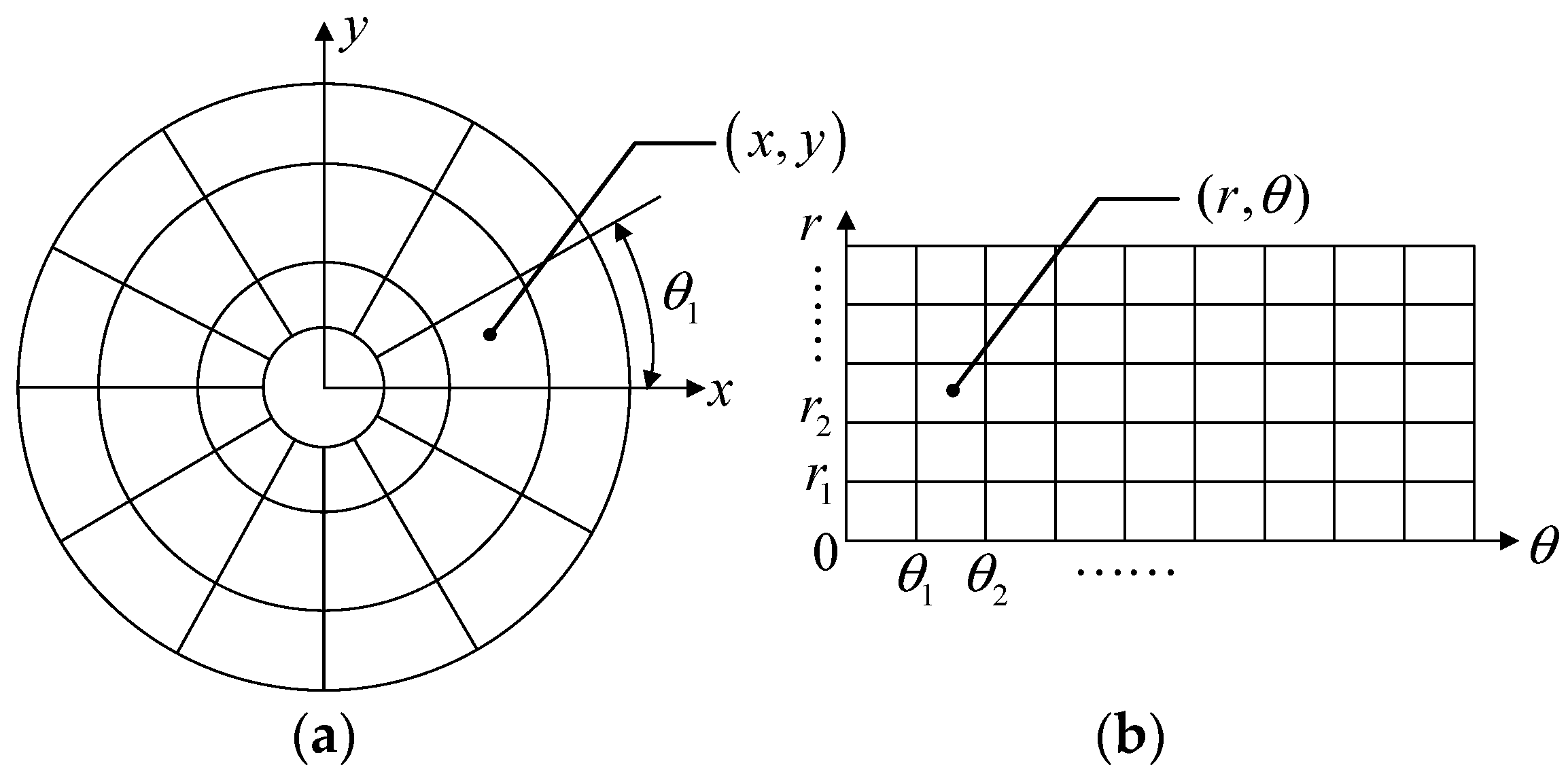
2.1. Log-Polar Transformation
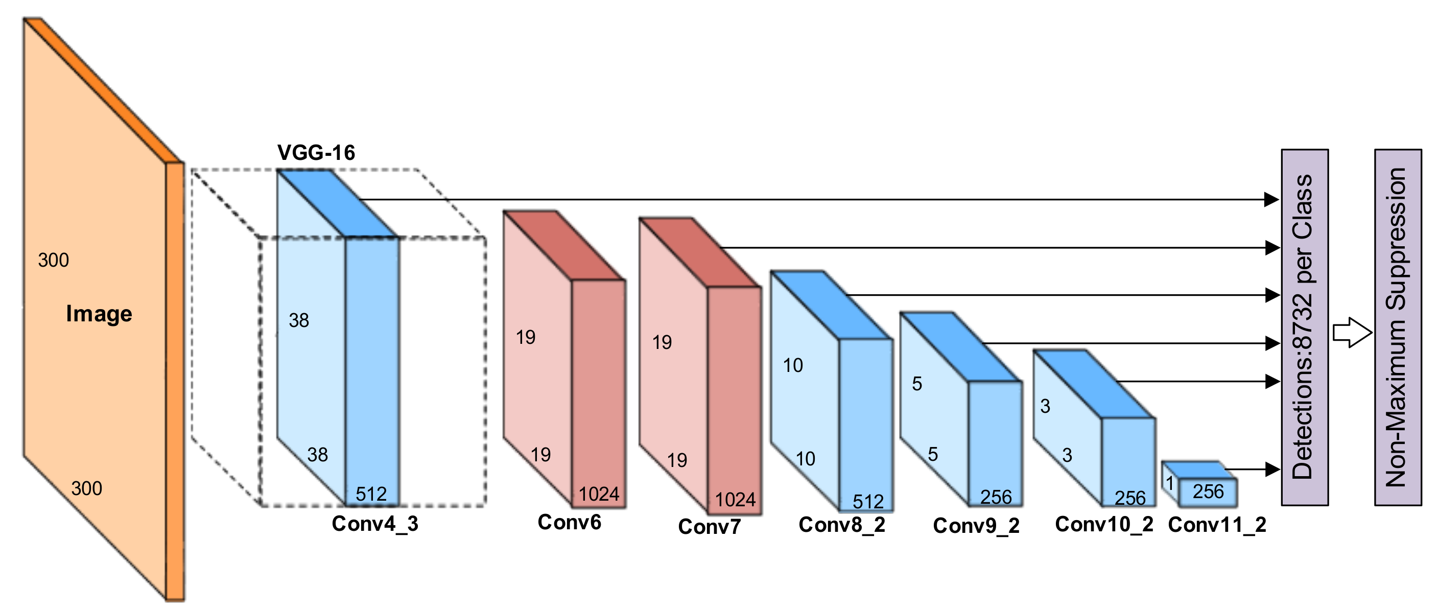
2.2. SSD300
3. LPNet
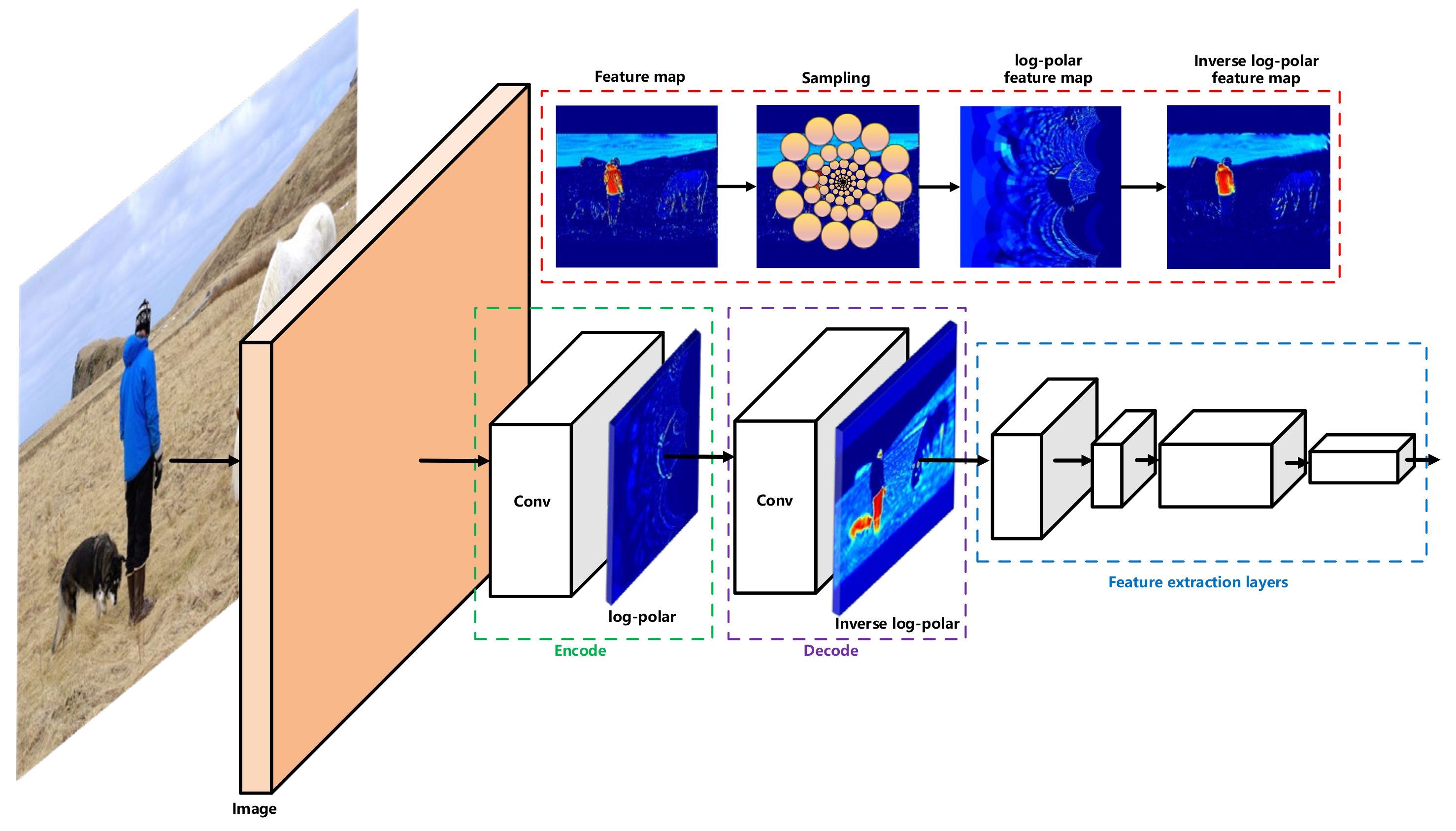
3.1. Architecture Overview
3.2. Sliding LPNet
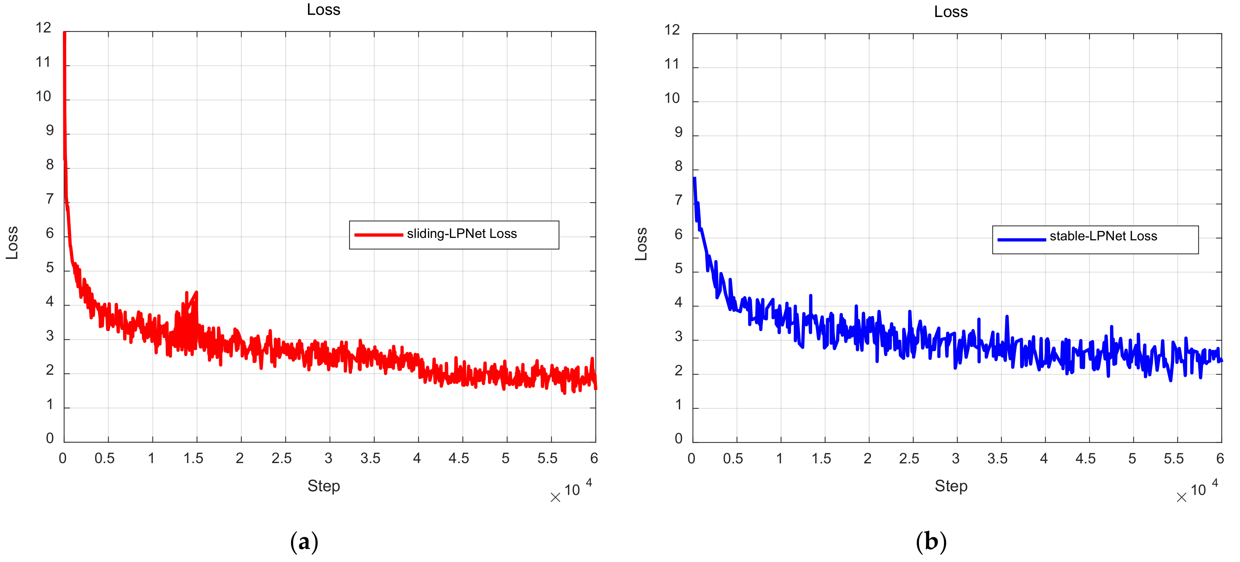
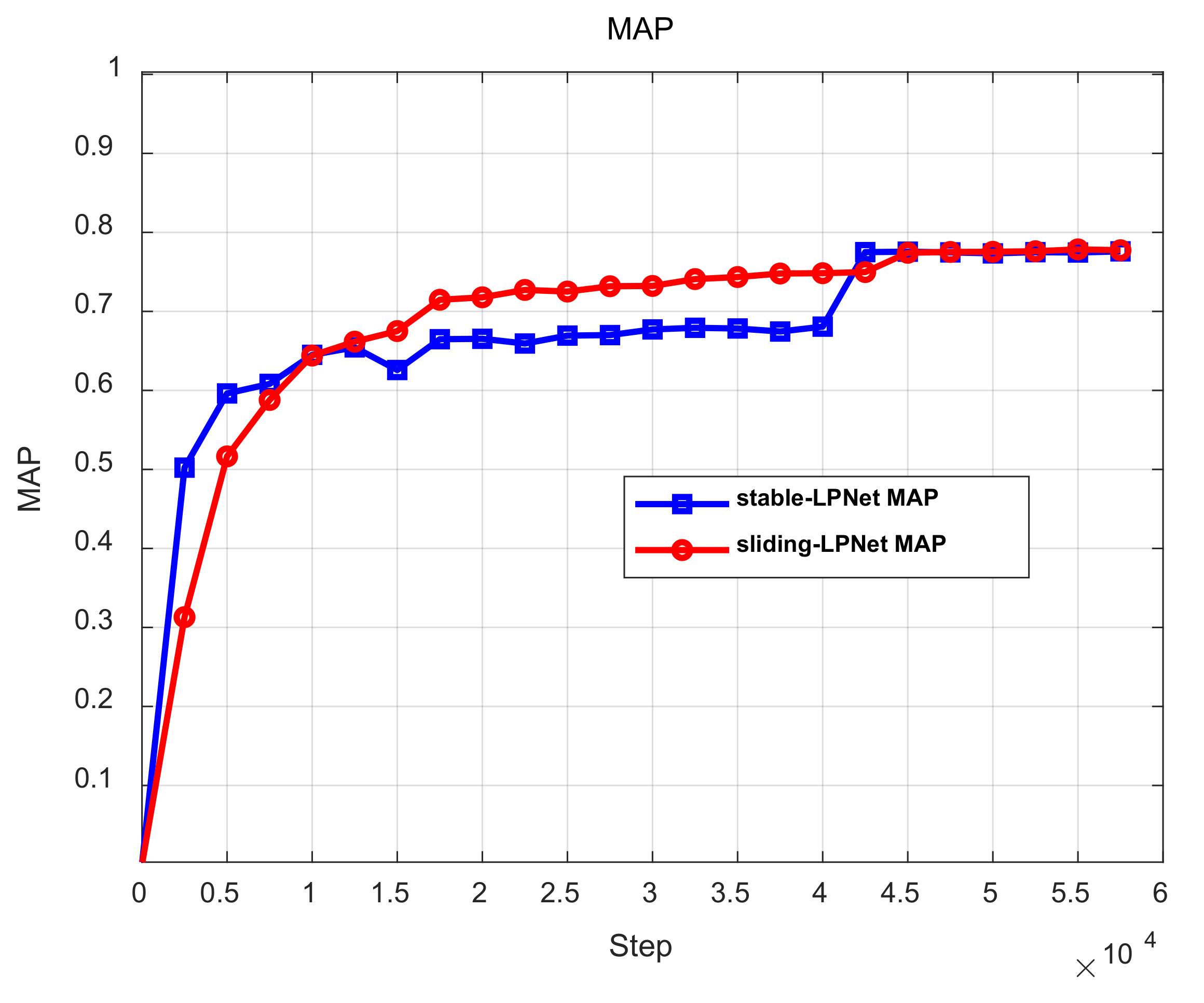
4. Experimental Results and Analysis
4.1. Experiment Setup
4.2. Results
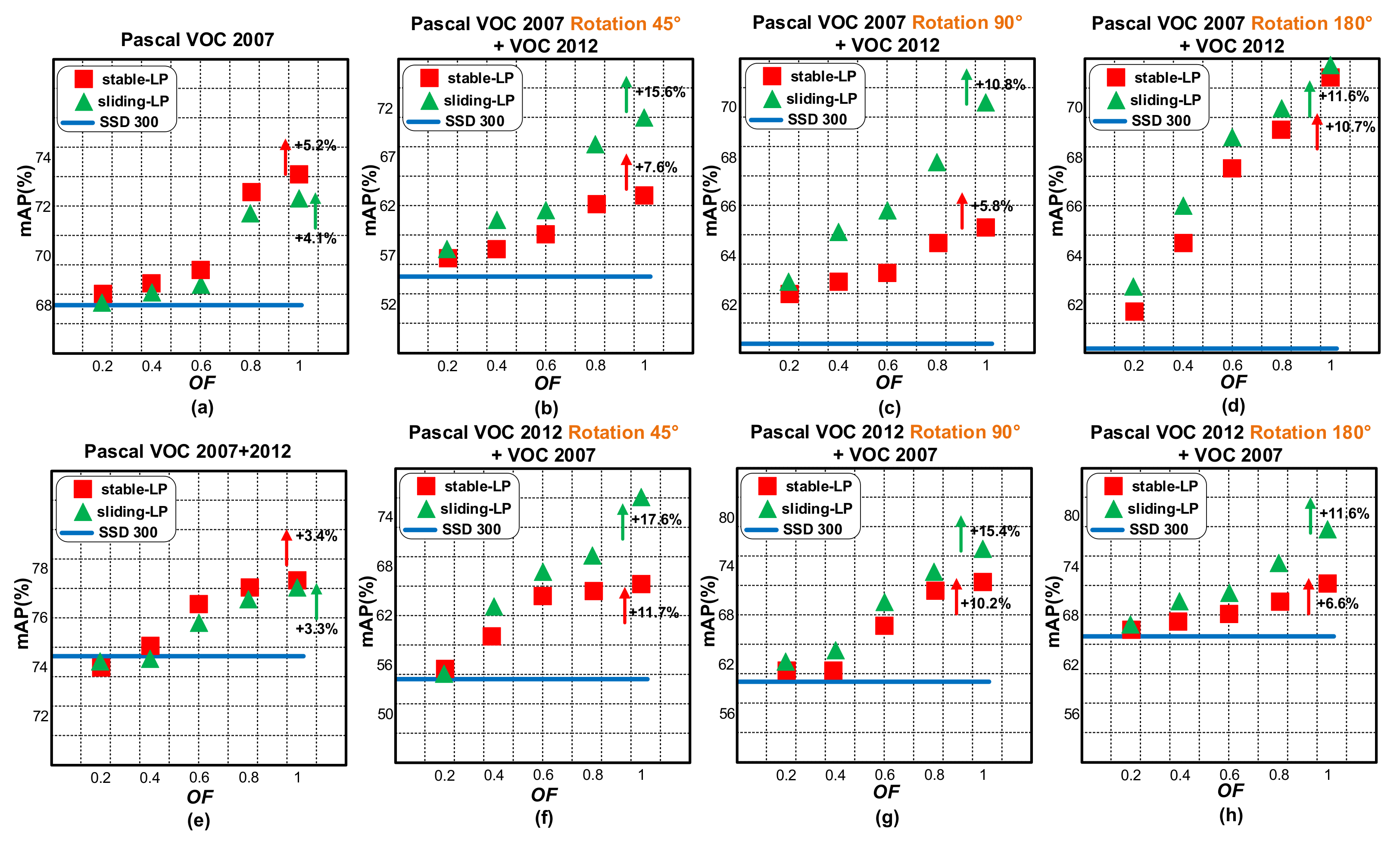
4.3. OF Impact
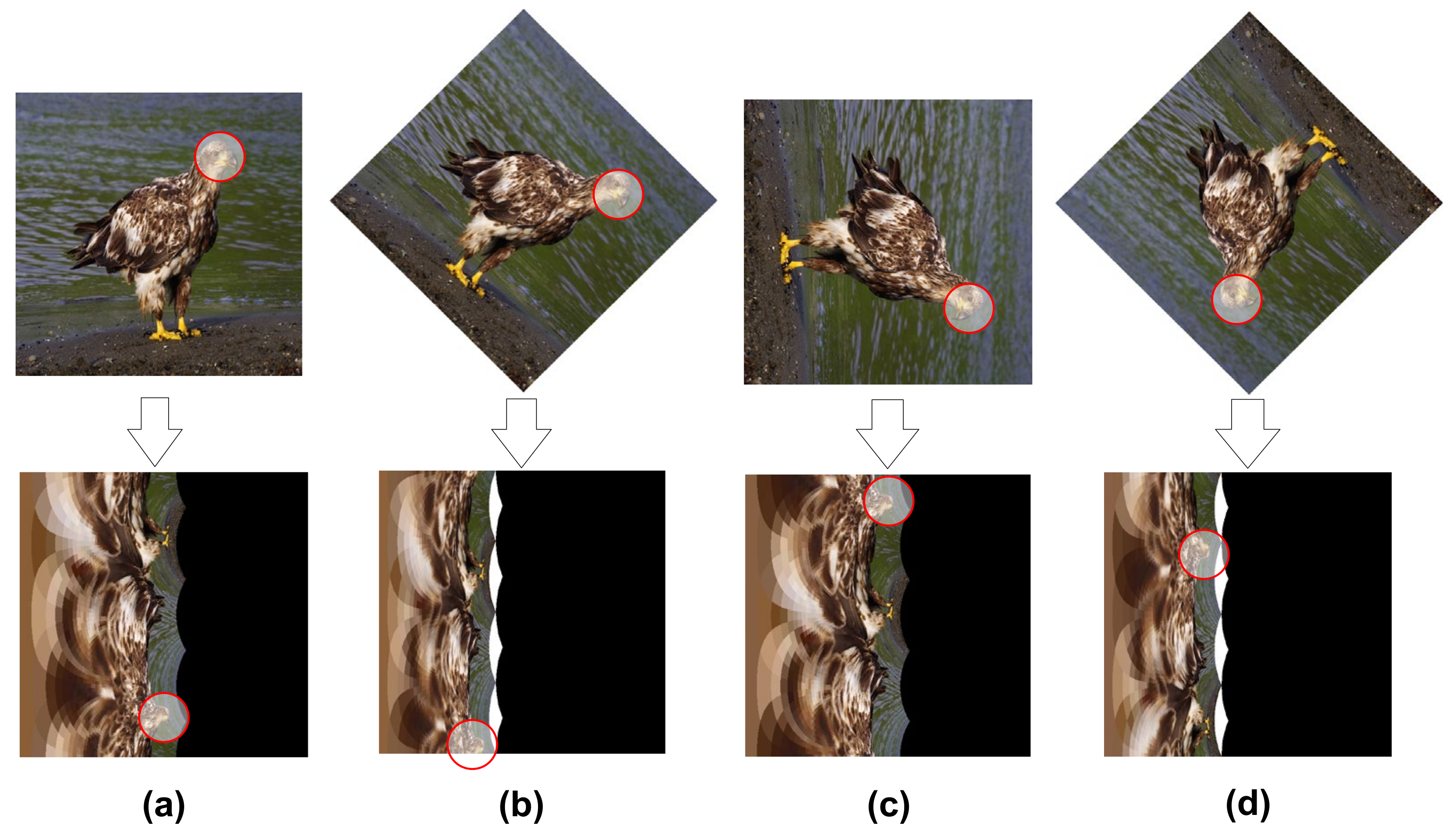
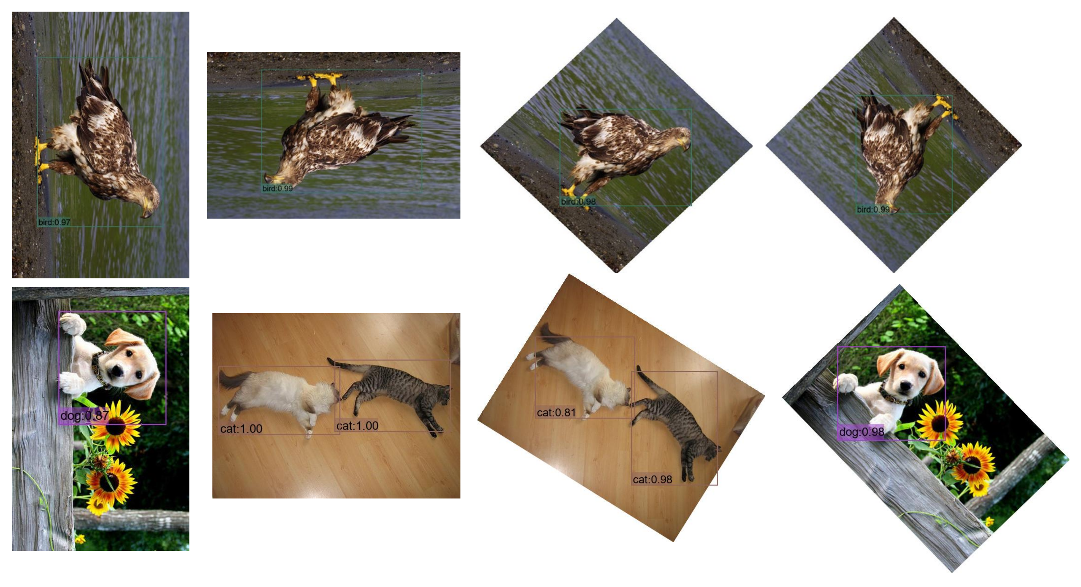
4.4. Dataset Rotation
5. Conclusions and Future Works
Author Contributions
Funding
Data Availability Statement
Conflicts of Interest
References
- LeCun, Y.; Bengio, Y.; Hinton, G.J. Deep learning. Nature 2015, 521, 436–444. [Google Scholar] [CrossRef] [PubMed]
- Xu, Z.; Lan, S.; Yang, Z.; Cao, J.; Wu, Z.; Cheng, Y.J.E. MSB R-CNN: A Multi-Stage Balanced Defect Detection Network. Electronics 2021, 10, 1924. [Google Scholar] [CrossRef]
- Kwon, H.; Kim, Y.; Yoon, H.; Choi, D. Classification score approach for detecting adversarial example in deep neural network. Multimed. Tools Appl. 2021, 80, 10339–10360. [Google Scholar] [CrossRef]
- Fu, C.; Xu, J.; Lin, F.; Guo, F.; Liu, T.; Zhang, Z. Object saliency-aware dual regularized correlation filter for real-time aerial tracking. IEEE Trans. Geosci. Remote Sens. 2020, 58, 8940–8951. [Google Scholar] [CrossRef]
- Li, Y.; Fu, C.; Huang, Z.; Zhang, Y.; Pan, J. Intermittent contextual learning for keyfilter-aware uav object tracking using deep convolutional feature. IEEE Trans. Multimed. 2020, 23, 810–822. [Google Scholar] [CrossRef]
- Ko, K.; Gwak, H.; Thoummala, N.; Kwon, H.; Kim, S. SqueezeFace: Integrative Face Recognition Methods with LiDAR Sensors. J. Sens. 2021, 2021, 4312245. [Google Scholar] [CrossRef]
- Jiao, S.; Gao, Y.; Feng, J.; Lei, T.; Yuan, X. Does deep learning always outperform simple linear regression in optical imaging. Opt. Express 2020, 28, 3717–3731. [Google Scholar] [CrossRef] [Green Version]
- Jiao, S.; Feng, J.; Gao, Y.; Lei, T.; Xie, Z.; Yuan, X. Optical Machine Learning with Single-pixel Imaging. In Adaptive Optics: Analysis, Methods & Systems; OSA: Washington, DC, USA, 2020; p. JW2A.43. [Google Scholar]
- Jiao, S.; Gao, Y.; Feng, J.; Lei, T.; Yuan, X. Outperformance of Linear-regression-based Methods over Deep Learning in Optical Imaging. In Digital Holography and Three-Dimensional Imaging; Optical Society of America: Washington, DC, USA, 2020; p. JW2A.42. [Google Scholar]
- Zaidi, B.F.; Selouani, S.A.; Boudraa, M.; Yakoub, M.S. Deep neural network architectures for dysarthric speech analysis and recognition. Neural Comput. Appl. 2021, 33, 9089–9108. [Google Scholar] [CrossRef]
- Song, Z.J. English speech recognition based on deep learning with multiple features. Computing 2020, 102, 663–682. [Google Scholar] [CrossRef]
- Bochkovskiy, A.; Wang, C.-Y.; Liao, H.Y.M. Yolov4: Optimal speed and accuracy of object detection. arXiv 2020, arXiv:2004.10934. [Google Scholar]
- Chessa, M.; Solari, F. Local feature extraction in log-polar images. In Proceedings of the International Conference on Image Analysis and Processing, Genova, Italy, 7–11 September 2015; pp. 410–420. [Google Scholar]
- Xie, X.; Cheng, G.; Wang, J.; Yao, X.; Han, J. Oriented R-CNN for Object Detection. In Proceedings of the IEEE/CVF International Conference on Computer Vision, Quebec, QC, Canada, 11–17 October 2021; pp. 3520–3529. [Google Scholar]
- Han, J.; Ding, J.; Xue, N.; Xia, G.S. Redet: A rotation-equivariant detector for aerial object detection. In Proceedings of the IEEE/CVF Conference on Computer Vision and Pattern Recognition, Nashville, TN, USA, 19–25 June 2021; pp. 2786–2795. [Google Scholar]
- Remmelzwaal, L.A.; Ellis, G.F.; Tapson, J.; Mishra, A.K. Biologically-inspired Salience Affected Artificial Neural Network (SANN). arXiv 2019, arXiv:1908.03532. [Google Scholar]
- Kim, J.; Sangjun, O.; Kim, Y.; Lee, M.J. Convolutional neural network with biologically inspired retinal structure. Procedia Comput. Sci. 2016, 88, 145–154. [Google Scholar] [CrossRef] [Green Version]
- Nikitin, V.V.; Andersson, F.; Carlsson, M.; Duchkov, A. Fast hyperbolic Radon transform represented as convolutions in log-polar coordinates. Geosciences 2017, 105, 21–33. [Google Scholar] [CrossRef] [Green Version]
- Schwartz, E.L. Spatial mapping in the primate sensory projection: Analytic structure and relevance to perception. Biol. Cybern. 1977, 25, 181–194. [Google Scholar] [CrossRef]
- Araujo, H.; Dias, J.M. An introduction to the log-polar mapping [image sampling]. In Proceedings of the II Workshop on Cybernetic Vision, Sao Carlos, Brazil, 9–11 December 1996; pp. 139–144. [Google Scholar]
- Ebel, P.; Mishchuk, A.; Yi, K.M.; Fua, P.; Trulls, E. Beyond cartesian representations for local descriptors. In Proceedings of the IEEE/CVF International Conference on Computer Vision, Soul, Korea, 27 October–2 November 2019; pp. 253–262. [Google Scholar]
- Wechsler, H. Neural Networks for Perception: Human and Machine Perception; Academic Press: Cambridge, MA, USA, 2014. [Google Scholar]
- Grosso, E.; Tistarelli, M. Log-polar stereo for anthropomorphic robots. In Proceedings of the European Conference on Computer Vision, Sao Carlos, Brazil, 12 October 2000; pp. 299–313. [Google Scholar]
- Massone, L.; Sandini, G.; Tagliasco, V. “Form-invariant” topological mapping strategy for 2D shape recognition. lGVIP 1985, 30, 169–188. [Google Scholar] [CrossRef]
- Jurie, F. A new log-polar mapping for space variant imaging: Application to face detection and tracking. Pattern Recognit. 1999, 32, 865–875. [Google Scholar] [CrossRef]
- Zokai, S.; Wolberg, G. Image registration using log-polar mappings for recovery of large-scale similarity and projective transformations. IEEE Trans. Image Process. 2005, 14, 1422–1434. [Google Scholar] [CrossRef]
- Yang, Z.-F.; Kuo, C.T.; Kuo, T.H. Authorization Identification by Watermarking in Log-polar Coordinate System. Comput. J. 2018, 61, 1710–1723. [Google Scholar] [CrossRef]
- Cheng, Y.; Cao, J.; Zhang, Y.; Hao, Q.J.B. Review of state-of-the-art artificial compound eye imaging systems. Bioinspir. Biomim. 2019, 14, 031002. [Google Scholar] [CrossRef]
- Yang, H.-y.; Qi, S.R.; Chao, W.; Yang, S.-b.; Wang, X.Y. Image analysis by log-polar Exponent-Fourier moments. Pattern Recognit. 2020, 101, 107177. [Google Scholar] [CrossRef]
- Ellahyani, A.; El Ansari, M.J. Mean shift and log-polar transform for road sign detection. Multimed. Tools Appl. 2017, 76, 24495–24513. [Google Scholar] [CrossRef]
- Worrall, D.E.; Garbin, S.J.; Turmukhambetov, D.; Brostow, G.J. Harmonic networks: Deep translation and rotation equivariance. In Proceedings of the IEEE Conference on Computer Vision and Pattern Recognition, Honolulu, HI, USA, 21–26 July 2017; pp. 5028–5037. [Google Scholar]
- Dumont, B.; Maggio, S.; Montalvo, P. Robustness of rotation-equivariant networks to adversarial perturbations. arXiv 2018, arXiv:1802.06627. [Google Scholar]
- Claveau, D.; Wang, C. Systems, A. Space-variant motion detection for active visual target tracking. Robot. Auton. Syst. 2009, 57, 11–22. [Google Scholar] [CrossRef] [Green Version]
- Wolberg, G.; Zokai, S. Robust image registration using log-polar transform. In Proceedings of the Proceedings 2000 International Conference on Image Processing (Cat. No. 00CH37101), Vancouver, BC, Canada, 10–13 September 2000; pp. 493–496. [Google Scholar]
- Zhang, X.; Liu, L.; Xie, Y.; Chen, J.; Wu, L.; Pietikainen, M. Rotation invariant local binary convolution neural networks. In Proceedings of the IEEE International Conference on Computer Vision Workshops, Venice, Italy, 22–29 October 2017; pp. 1210–1219. [Google Scholar]
- Esteves, C.; Allen-Blanchette, C.; Zhou, X.; Daniilidis, K. Polar transformer networks. arXiv 2017, arXiv:1709.01889. [Google Scholar]
- Amorim, M.; Bortoloti, F.; Ciarelli, P.M.; de Oliveira, E.; de Souza, A.F. Analysing rotation-invariance of a log-polar transformation in convolutional neural networks. In Proceedings of the 2018 International Joint Conference on Neural Networks (IJCNN), Rio de Janeiro, Brazil, 8–13 July 2018; pp. 1–6. [Google Scholar]
- Kiritani, T.; Ono, K. Recurrent Attention Model with Log-Polar Mapping is Robust against Adversarial Attacks. arXiv 2020, arXiv:2002.05388. [Google Scholar]
- Remmelzwaal, L.A.; Mishra, A.K.; Ellis, G.F. Human eye inspired log-polar pre-processing for neural networks. In Proceedings of the 2020 International SAUPEC/RobMech/PRASA Conference, Cape Town, South Africa, 29–31 January 2020; pp. 1–6. [Google Scholar]
- Traver, V.J.; Bernardino, A.J.R.; Systems, A. A review of log-polar imaging for visual perception in robotics. Robot. Auton. Syst. 2010, 58, 378–398. [Google Scholar] [CrossRef]
- Matuszewski, D.J.; Hast, A.; Wählby, C.; Sintorn, I.M. A short feature vector for image matching: The Log-Polar Magnitude feature descriptor. PLoS ONE 2017, 12, e0188496. [Google Scholar]
- Hu, B.; Zhang, Z.J.N.C. Bio-inspired visual neural network on spatio-temporal depth rotation perception. Neural Comput. Appl. 2021, 1–20. [Google Scholar] [CrossRef]
- Gamba, P.; Lombardi, L.; Porta, M. Log-map analysis. Parallel Comput. 2008, 34, 757–764. [Google Scholar] [CrossRef]
- Lombardi, L.; Porta, M. Log-map analysis. In Visual Attention Mechanisms; Springer: Boston, MA, USA, 2002; pp. 41–51. [Google Scholar]
- Li, D.D.; Wen, G.; Kuai, Y.; Zhang, X.J. Log-polar mapping-based scale space tracking with adaptive target response. J. Electron. Imaging 2017, 26, 033003. [Google Scholar] [CrossRef]
- Liu, W.; Anguelov, D.; Erhan, D.; Szegedy, C.; Reed, S.; Fu, C.Y.; Berg, A.C. Ssd: Single shot multibox detector. In Proceedings of the European Conference on Computer Vision, Amsterdam, The Netherlands, 11–14 October 2016; pp. 21–37. [Google Scholar]
- Ren, S.; He, K.; Girshick, R.; Sun, J. Faster r-cnn: Towards real-time object detection with region proposal networks. Adv. Neural Inf. Process. Syst. 2015, 28, 91–99. [Google Scholar] [CrossRef] [PubMed] [Green Version]
- Redmon, J.; Divvala, S.; Girshick, R.; Farhadi, A. You only look once: Unified, real-time object detection. In Proceedings of the IEEE Conference on Computer Vision and Pattern Recognition, Las Vegas, NV, USA, 27–30 June 2016; pp. 779–788. [Google Scholar]
- Girshick, R. Fast r-cnn. In Proceedings of the IEEE International Conference on Computer Vision, Santiago, Chile, 7–13 December 2015; pp. 1440–1448. [Google Scholar]


| Location | Value | Location | Value | Location | Value |
|---|---|---|---|---|---|
| (x1,y1) | (50,50) | (x4,y4) | (50,150) | (x7,y7) | (50,250) |
| (x2,y2) | (150,50) | (x5,y5) | (150,150) | (x8,y8) | (150,250) |
| (x3,y3) | (250,50) | (x6,y6) | (250,150) | (x9,y9) | (250,250) |
| Method | mAP | Aero | Bike | Bird | Boat | Bottle | Bus | Car | Cat | Chair | Cow | Table | Dog | Horse | mBike | Person | Plant | Sheep | Sofa | Train | Tv |
|---|---|---|---|---|---|---|---|---|---|---|---|---|---|---|---|---|---|---|---|---|---|
| LPNet(sliding) | 77.6 | 81.8 | 84.5 | 76.2 | 71.9 | 49.4 | 85.9 | 86.3 | 87.5 | 62.0 | 81.6 | 73.9 | 86.1 | 85.8 | 84.1 | 79.8 | 53.7 | 78.4 | 80.8 | 85.7 | 76.7 |
| LPNet(stable) | 77.7 | 82.8 | 83.8 | 75.7 | 71.0 | 51.1 | 86.0 | 86.1 | 88.3 | 62.7 | 81.5 | 84.2 | 86.2 | 87.3 | 84.2 | 79.5 | 53.3 | 77.7 | 80.7 | 85.3 | 77.2 |
| SSD300 [46] | 74.3 | 75.5 | 80.2 | 72.3 | 66.3 | 47.6 | 83.3 | 84.2 | 86.1 | 54.7 | 78.3 | 73.9 | 84.5 | 85.3 | 82.6 | 76.2 | 48.6 | 73.9 | 76.0 | 83.4 | 74.0 |
| Faster [47] | 73.2 | 76.5 | 79.0 | 70.9 | 65.5 | 52.1 | 83.1 | 84.7 | 86.4 | 52.0 | 81.9 | 65.7 | 84.8 | 84.6 | 77.5 | 76.7 | 38.8 | 73.6 | 73.9 | 83.0 | 72.6 |
| Fast [49] | 70.0 | 77.0 | 78.1 | 69.3 | 59.4 | 38.3 | 81.6 | 78.6 | 86.7 | 42.8 | 78.8 | 68.9 | 84.7 | 82.0 | 76.6 | 69.9 | 31.8 | 70.1 | 74.8 | 80.4 | 70.4 |
| OF | 0.1 | 0.2 | 0.3 | 0.4 | 0.5 | 0.6 | 0.7 | 0.8 | 0.9 | 1.0 |
|---|---|---|---|---|---|---|---|---|---|---|
| sliding LPNet (mAP) | 75.2 | 75.8 | 76.1 | 76.3 | 76.5 | 76.6 | 76.9 | 77.2 | 77.5 | 77.6 |
| stable LPNet (mAP) | 75.4 | 75.9 | 76.3 | 76.4 | 76.8 | 77.1 | 77.3 | 77.6 | 77.6 | 77.7 |
Publisher’s Note: MDPI stays neutral with regard to jurisdictional claims in published maps and institutional affiliations. |
© 2021 by the authors. Licensee MDPI, Basel, Switzerland. This article is an open access article distributed under the terms and conditions of the Creative Commons Attribution (CC BY) license (https://creativecommons.org/licenses/by/4.0/).
Share and Cite
Cao, J.; Bao, C.; Hao, Q.; Cheng, Y.; Chen, C. LPNet: Retina Inspired Neural Network for Object Detection and Recognition. Electronics 2021, 10, 2883. https://doi.org/10.3390/electronics10222883
Cao J, Bao C, Hao Q, Cheng Y, Chen C. LPNet: Retina Inspired Neural Network for Object Detection and Recognition. Electronics. 2021; 10(22):2883. https://doi.org/10.3390/electronics10222883
Chicago/Turabian StyleCao, Jie, Chun Bao, Qun Hao, Yang Cheng, and Chenglin Chen. 2021. "LPNet: Retina Inspired Neural Network for Object Detection and Recognition" Electronics 10, no. 22: 2883. https://doi.org/10.3390/electronics10222883