Multi-Method Analysis of Medical Records and MRI Images for Early Diagnosis of Dementia and Alzheimer’s Disease Based on Deep Learning and Hybrid Methods

Abstract

Dementia and Alzheimer’s disease are caused by neurodegeneration and poor communication between neurons in the brain. So far, no effective medications have been discovered for dementia and Alzheimer’s disease. Thus, early diagnosis is necessary to avoid the development of these diseases. In this study, efficient machine learning algorithms were assessed to evaluate the Open Access Series of Imaging Studies (OASIS) dataset for dementia diagnosis. Two CNN models (AlexNet and ResNet-50) and hybrid techniques between deep learning and machine learning (AlexNet+SVM and ResNet-50+SVM) were also evaluated for the diagnosis of Alzheimer’s disease. For the OASIS dataset, we balanced the dataset, replaced the missing values, and applied the t-Distributed Stochastic Neighbour Embedding algorithm (t-SNE) to represent the high-dimensional data in the low-dimensional space. All of the machine learning algorithms, namely, Support Vector Machine (SVM), Decision Tree, Random Forest and K Nearest Neighbours (KNN), achieved high performance for diagnosing dementia. The random forest algorithm achieved an overall accuracy of 94% and precision, recall and F1 scores of 93%, 98% and 96%, respectively. The second dataset, the MRI image dataset, was evaluated by AlexNet and ResNet-50 models and AlexNet+SVM and ResNet-50+SVM hybrid techniques. All models achieved high performance, but the performance of the hybrid methods between deep learning and machine learning was better than that of the deep learning models. The AlexNet+SVM hybrid model achieved accuracy, sensitivity, specificity and AUC scores of 94.8%, 93%, 97.75% and 99.70%, respectively.

1. Introduction

The number of dangerous diseases has increased in recent years due to demographic shifts in developing and developed countries [1]. Despite advances in medical techniques, effective treatments for dementia and Alzheimer’s disease remain elusive, except for some drugs that delay the diseases’ progression. Therefore, early diagnosis plays an important role in stopping the progression of the diseases to their advanced stages [1,2]. Some of the severe chronic conditions that have attracted much attention in the field of mental health are dementia and Alzheimer’s diseases because of their widespread prevalence among the elderly and their harmful effects on the elderly’s cognitive abilities to conduct daily activities normally. Dementia is the loss or impairment of memory to conduct healthy mental abilities due to age or disease; it is characterised by changes in the mind and behavioural disturbance or stroke. It is a syndrome that includes impaired memory, behaviour and thinking and the loss of ability to perform daily activities [3,4]. According to the reports of the World Health Organization (WHO), about 47 million people suffer from dementia around the world, and the number is rapidly increasing annually; the number of sufferers could reach 82 million people by 2030. The underlying causes of dementia are neurodegeneration and weak brain connectivity, which lead to poor decision-making; the non-neurodegenerative mechanisms result in vascular dementia. Alzheimer’s disease (AD) is one of the most common and prevalent types of dementia and accounts for 60% to 70% of dementia cases. Age is the direct cause of AD, especially in people over the age of 65. AD has a more noticeable prevalence among women than men. However, AD aetiology has not yet been identified. The main hypotheses are based on the accumulation of extracellular A$\beta$ peptides and the accumulation of hyperphosphorylated tau proteins inside brain cells. These two structures are biomarkers called amyloid plaques (an accumulation of beta-amyloid fragments between neurons) and tangles (intracellular accumulations of tau protein in the form of twisted fibrils). A biomarker is a measure or indicator of the brain’s biological state. Biomarkers appear early before clinical symptoms appear [5]. Thus, as a histopathological procedure, the accumulation of amyloid plaques and neurofibrillary tangles is responsible for neuronal damage and death [6,7], thereby leading to progressive memory loss with physiological changes in thinking and behaviour. Dementia and Alzheimer’s are multifactorial diseases that occur independently from physiological aging parameters, such as diet, sleep disturbances, environmental factors, sedentary lifestyle and genetic predisposition.

AD is one of the main causes of intellectual disability among the elderly worldwide. At the onset of AD, a combination of psychological and mental evaluation occurs, such as that involving tau protein and cerebrovascular amyloid protein, to find synapses, brain plaques and neuronal degeneration. There are measures to assess cognitive and mental decline in the elderly, such as tacrine for the level of symptoms and assessment of genetic history to identify Down syndrome [8,9]. AD is then evaluated by a brain imaging called Pittsburgh Compound B (PIB), which is based on n-positron emission tomography (PET); it is considered for the early detection and monitoring of AD [10,11]. Subsequently, the AD Neuroimaging Initiative (ADNI) is established; it standardises image formats with psychological and intellectual tests to monitor the effectiveness of treatment and early detection of disease. There is an urgent need to identify biomarkers that can detect histological changes in the brain, which may indicate neurological disorders, such as atrophy and amyloid plaques; these changes may represent early signs of dementia, and AD can be predicted. Thus, biomarkers help us differentiate between dementia and AD and predict them early. In recent years, researchers have provided biomarkers in the form of neuroimaging techniques, such as MRI, single-photon emission computed tomography (SPECT) and Positron Emission Tomography (PET), which had a prominent role in the early diagnosis of both dementia and Alzheimer’s [12]. Diagnosing the soft tissues of the brain and distinguishing them from healthy tissues are essential for the early prediction of dementia and AD. Manually extracting features from MRI images or medical records requires a great deal of time and effort from experts. 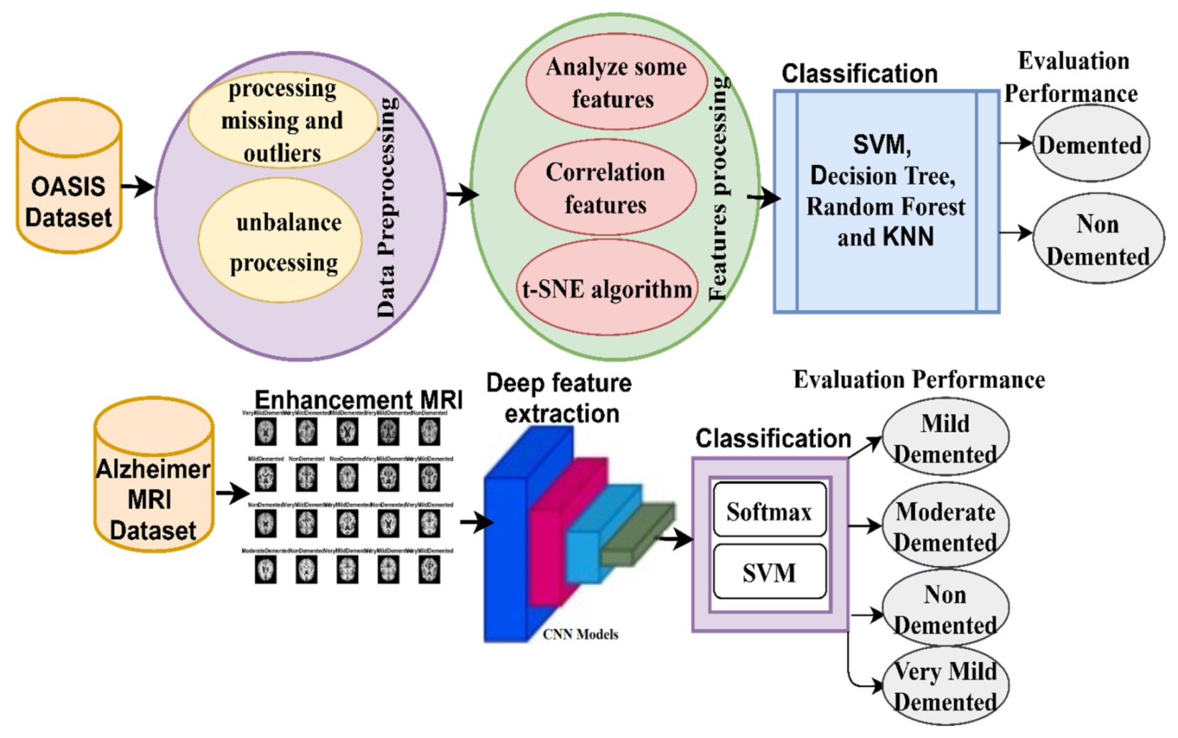Similarities between soft and healthy tissues in MRI make manual diagnosis more prone to errors [13]. Therefore, this paper aimed to evaluate the use of machine learning algorithms on the Open Access Series of Imaging Studies (OASIS) dataset for the early prediction of dementia and the use of deep learning algorithms and hybrid techniques between deep and machine learning on MRI dataset for the early prediction of AD and for differentiating disease stages and severity from mild to moderate to severe. Machine learning, deep learning and hybrid and pattern analysis technologies serve as powerful tools for building predictive models based on MRI images and medical records for computer-aided diagnosis. Deep learning techniques extract deep representative feature maps without the need for manual feature representation. All results are more effective, consistent, less likely to create bias and proven to be effective in diagnosing dementia and AD compared with manual approaches.

Duc et al. introduced a deep learning-based method for assessing Mini-Mental State Examination (MMSE) through resting-state functional Magnetic Resonance Imaging (rs-fMRI); the system yielded good results for the diagnosis of AD [14]. Li et al. presented a deep learning model and validated the diagnosis of 2146 cases of magnetic resonance imaging to predict the progression of mild cognitive impairment (MCI) to AD dementia [15]. Francesco et al. introduced deep learning techniques to evaluate an EEG dataset to distinguish Creutzfeldt–Jakob disease from other dementias. The method is based on the extraction of time frequencies from EEG by continuous wavelet transform (CWT) algorithm and measuring complex EEG signals through permutation entropy (PE) [16]. Amoroso et al. applied the random forest technique to select the most important features extracted from the dataset that contains four classes, namely, HC, AD, MCI and cMCI, and their classification by DNN techniques [17]. Popuri et al. presented a model calculating the FDG-PET DAT score (FPDS) as a score between 0 and 1 for the diagnosis of dementia of Alzheimer’s type (DAT) [18]. Raza et al. introduced a system for diagnosing AD and monitoring similar diseases through machine learning techniques [19]. Aram et al. presented several machine learning algorithms to evaluate the MMSE-KC and CERAD-K datasets for the diagnosis of dementia. The MMSE-KC dataset was diagnosed as normal or abnormal, whereas the CERAD-K dataset was diagnosed as both dementia and mild cognitive impairment [20]. Chen et al. introduced many machine learning algorithms and statistical methods for diagnosing people with dementia or no dementia; among these, Bayesian and SVM algorithms achieved the best performance [21]. Joshi et al. applied machine learning and deep learning methods to diagnose dementia. The system achieved the best accuracy when collecting tests for both machine and deep learning [22]. Cho et al. introduced a double-layer hierarchical architecture for the early diagnosis of dementia. The Bayesian algorithm runs at the top layer, whereas the FCM and PNN algorithms run at the base layer [23]. Trambaiolli et al. presented an SVM algorithm to evaluate the electroencephalography (EEG) dataset to classify EEG signals as normal and Alzheimer’s images. The SVM algorithm achieved an accuracy of 87% [24]. Shanklea et al. presented a machine learning algorithm to predict CDR; the Naive Bayes algorithm achieved the highest accuracy among all algorithms [25]. Ekin et al. presented a 3D VGG convolutional neural network to preserve 3D MRI images while converting them to 2D through convolutional layers. The system was evaluated by using the ADNI and OASIS datasets, and the system achieved an accuracy of 73.4% for the ADNI dataset and an accuracy of 69.9% for the OASIS dataset [26]. Pinaya et al. presented standardised module-based autoencoder models for a neuroimaging dataset for AD diagnosis and trained an independent dataset on autoencoder modules. Then, they monitored the deviation of each patient and identified the deviated brain regions based on the autoencoder units [27]. Jorge et al. presented a spatio-temporal LME method based on Linear Mixed Effects (LME). The method exploits the spatial structure of MRI images to analyse measurements on the cortical surface. The method achieved good results [28]. The main contributions to this study are as follows:

First, for the OASIS dataset:

• Distribution of the converted class records to the non-demented and demented classes based on a feature value of CRD.
• Representation of high-dimensional data in low-dimensional data space by the t-SNE algorithm.
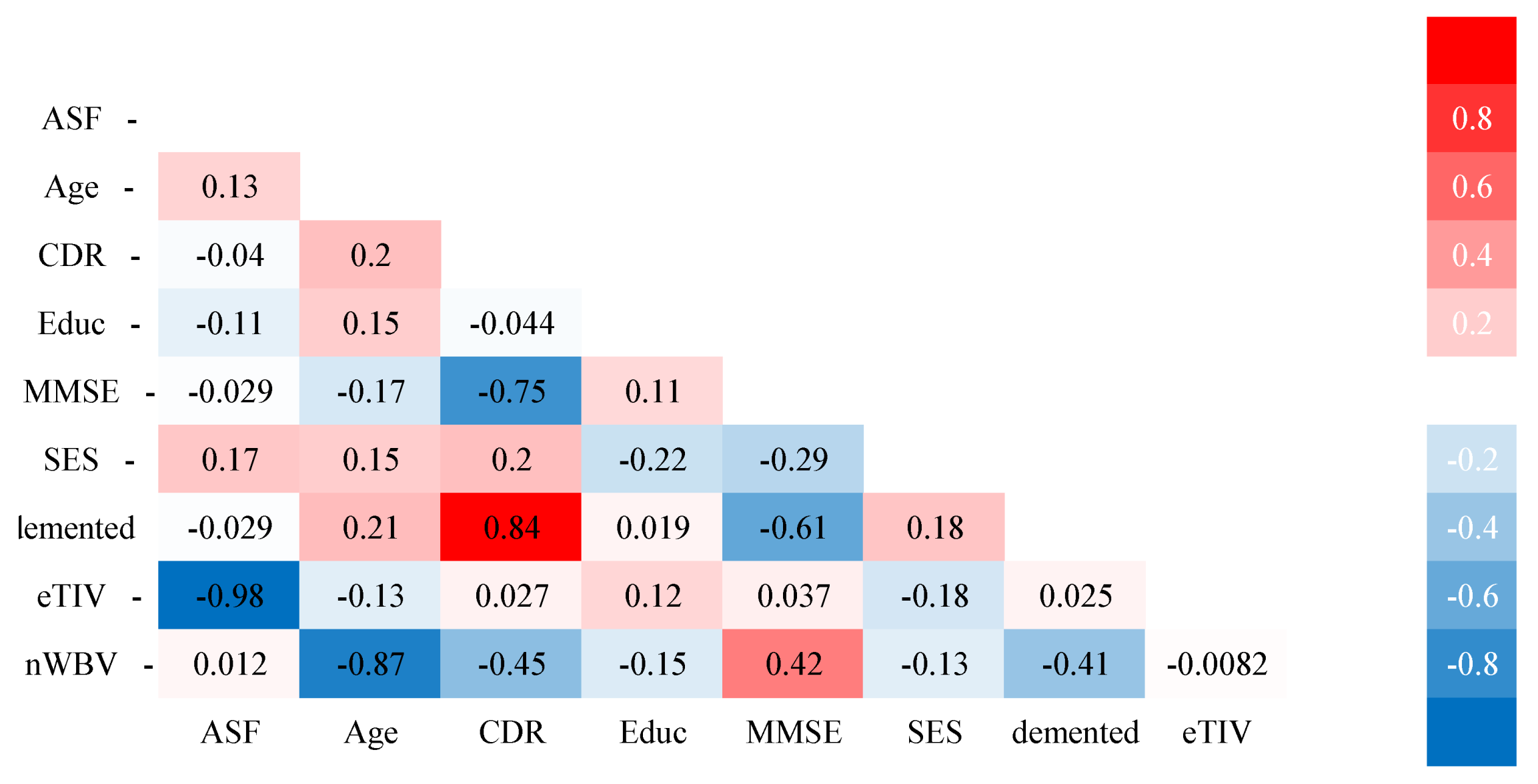
• Representation of the correlation of each feature with the other and the correlation of each feature with the target feature.

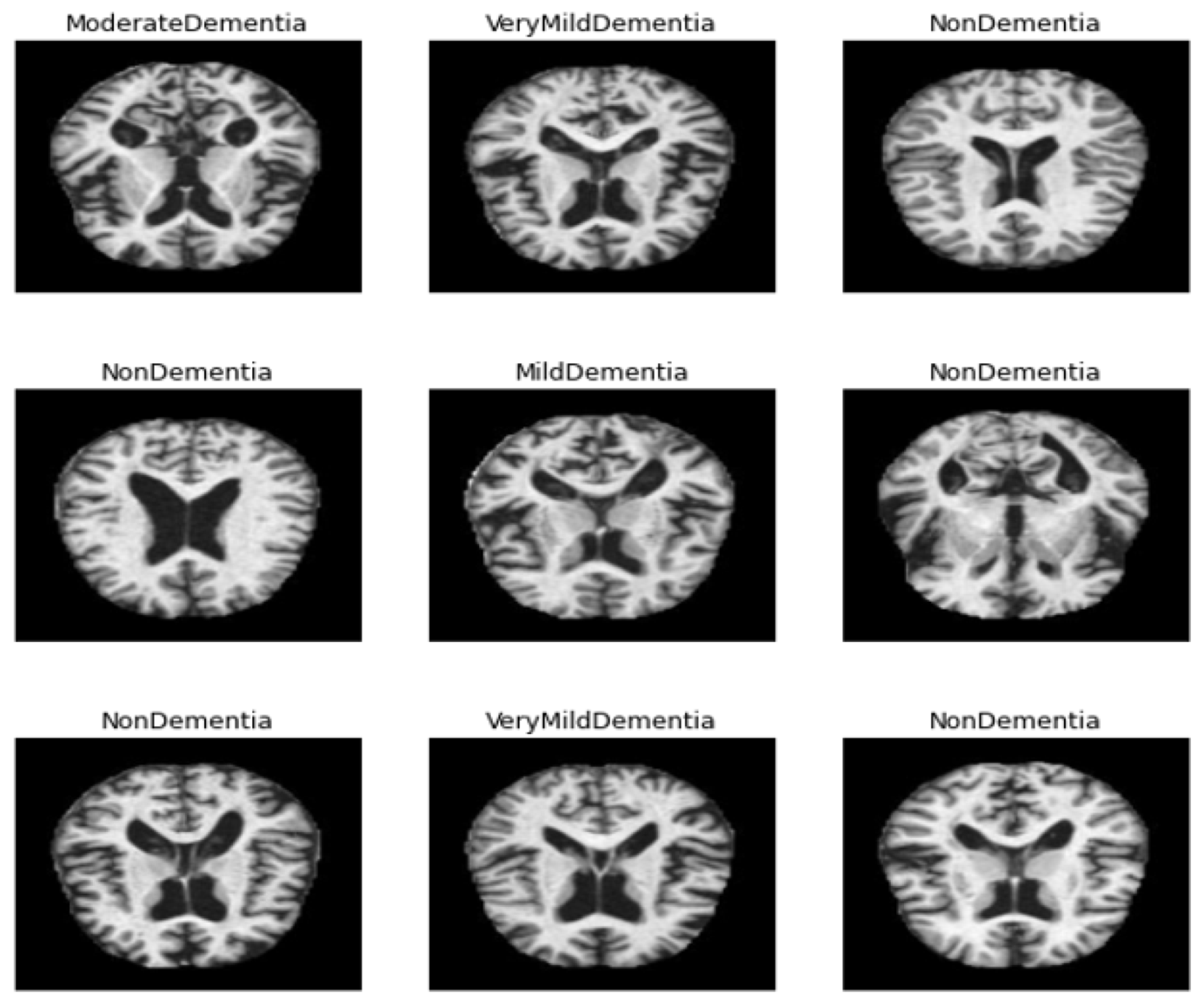
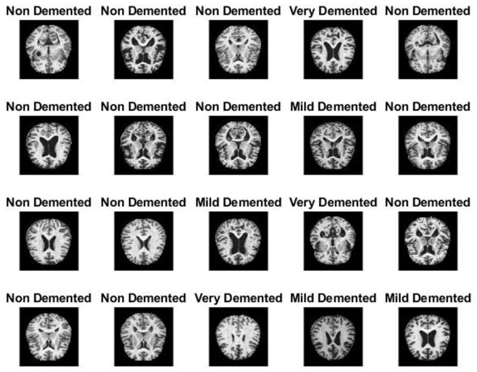
Second, for the MRI dataset:

• Balance the dataset by data augmentation technique to multiply the minority classes.
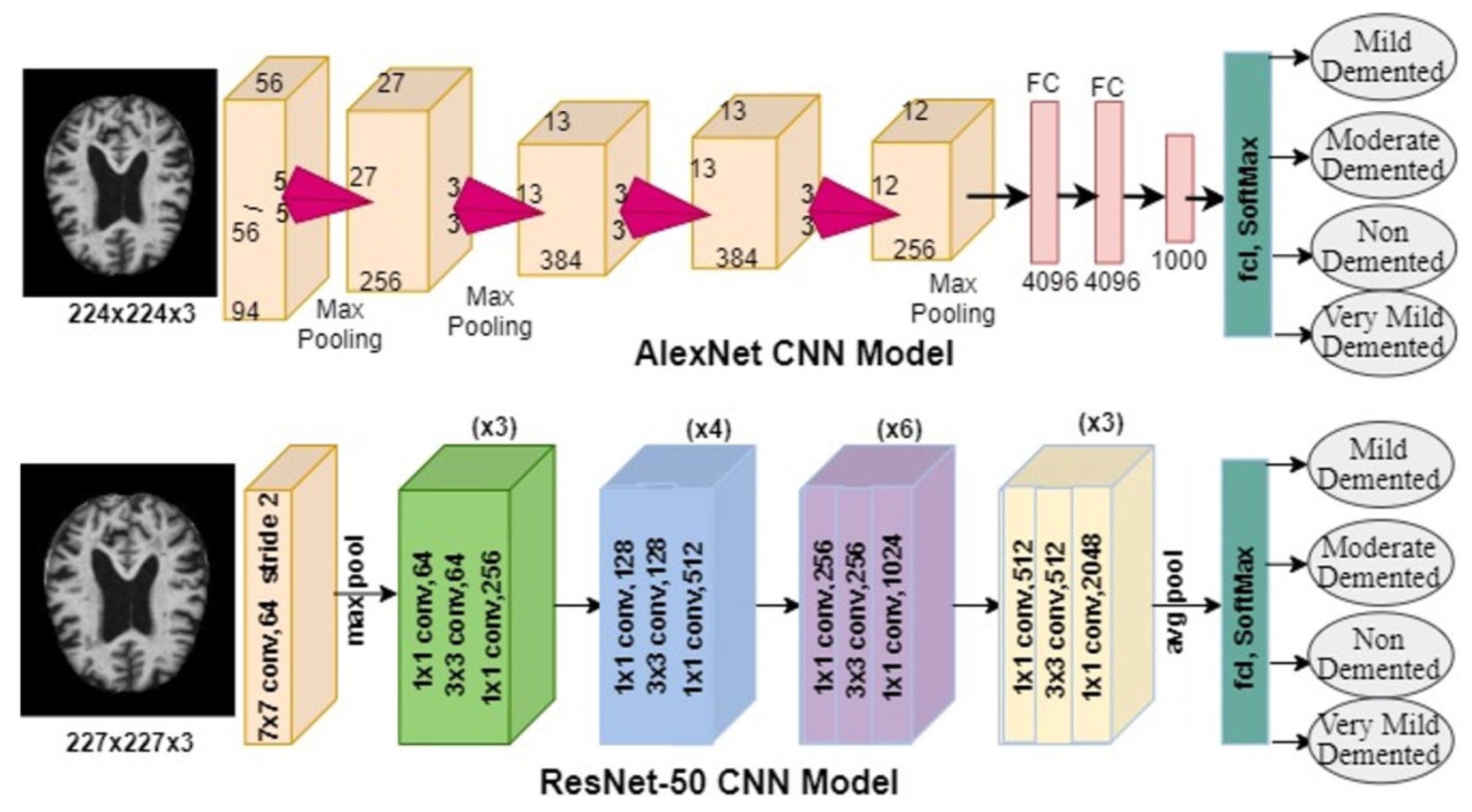
• Apply hybrid techniques between deep learning based on AlexNet and ResNet-50 models and machine learning based on SVM classifier to produce hybrid AlexNet+SVM and ResNet-50+SVM models that achieve high performance and effective diagnosis of AD.
• Machine learning, deep learning and hybrid techniques can be generalised with high efficiency to diagnose dementia and AD with the help of clinicians and experts and support their diagnostic decisions.

The remainder of the paper is organised as follows. Section 2 describes materials and methods and contains subsections for describing the two datasets and processing features. Section 3 reviews classification techniques. Section 4 presents the results of the analysis and diagnosis. Section 5 is the conclusion of the paper.

2. Materials and Methods

In this section, we describe the methodology used to process the OASIS and MRI datasets. The OASIS dataset contains medical records and is used for predicting dementia, whereas the MRI dataset is a made up of images for mild, moderate and severe AD. Figure 1 describes the methodology used to evaluate the proposed systems on the two datasets.

2.1. Description of Two Datasets

In this study, two datasets were used. The first dataset is called OASIS, which contains a combination of medical and environmental examinations (medical records) for the early detection of dementia. The second dataset is MRI, which relies on magnetic resonance imaging of the brain for the early detection of AD.

2.1.1. OASIS Dataset

OASIS dataset is an organisation that aims to make neuroimaging data of the brain available to researchers and interested parties. The OASIS-Cross-sectional [5] and OASIS-Longitudinal [6] datasets extracted from neuroanatomical atlases of MRI images are available. OASIS is a longitudinal neuroimaging and cross-sectional biomarker for normal and AD patients. The dataset is available in XML format and contains clinical and demographic data from MRI imaging. More details on the characteristics of the images and nomenclature can be obtained at http://www.oasis-brains.org/longitudinal_facts.html (accessed on 25 May 2021). The oasis_longitudinal dataset contains 15 features of 374 patients aged between 60 and 90 years old, of whom 37 are converted, 190 are demented and 147 are non-demented.

Table 1. Description of the OASIS dataset for the diagnosis of dementia.

No	Information	Features Name	Explanation
1	Gen Info	Subject.ID	A unique identifier for each patient
2		MRI.ID	A unique identifier for the MRI image of each patient
3		Group	The dataset is divided into converted (it was normal and turned into a dementia patient), demented and normal
4		Visit	Number of patient visits to detect dementia
5		MR.Delay	Not Known
6	Demographics	M.F	Gender (M or F)
7	Info	Hand	Right hand
8		Age	Age in years
9		EDUC	Years of education
10		SES	Socioeconomic status of each patient classified according to the Hollingshead Index of social status, which classifies from 1 as the highest status to 5 as the lowest status
11	Clinical Info	MMSE	Mini Mental state Examination score ranging from 0 as the worst to 30 as the best
12		CDR	Clinical Dementia Rating divided into 0 as no dementia, 0.5 as very mild Alzheimer’s Disease (AD), 1 as mild AD and 2 as moderate AD
13	Derived anatomic	eTIV	Estimated total intracranial volume (mm3)
14	volumes	nWBV	Normalised whole-brain volume expressed as a percentage of pixels in the atlas and categorised as white or grey matter by tissue segmentation
15		ASF	Atlas scaling factor. This is a computed scaling factor that works to convert the original space brain into the Atlas target

describes the dataset, which contains 15 features of 373 patients, including their demographics, clinical and derived anatomic volumes of information.

2.1.2. MRI Alzheimer’s Dataset

The MRI dataset for AD was obtained from the open source Kaggle website. The MRI dataset contains 6400 images separated into four classes, namely, mild dementia disease (896 images), moderate dementia disease (64 images), non-dementia (3200 images) and very mild dementia disease (2240 images) [29]. Figure 2 describes a sample of the MRI dataset for AD. https://www.kaggle.com/tourist55/alzheimers-dataset-4-class-of-images (accessed on 25 May 2021).

2.2. Pre-Processing

One of the most critical processes in data mining and medical image processing is pre-processing. This step transforms raw data into usable information, eliminates noise, processes missing numbers and enhances image quality. In this paper, we used data mining optimisation techniques to improve the OASIS dataset, whereas medical image processing optimisation techniques were used to improve the second dataset containing MRI images.

2.2.1. Pre-Processing of OASIS Dataset

Data cleaning, which involves removing outliers and replacing missing values, is one of the most important steps in data mining. At this stage, we looked at the overall distribution of the numerical and category columns to see which features can help our analysis; these features should not be strongly correlated with the target feature. We also looked at features that have a unique value to remove them. Afterwards, we addressed missing values and datatype mismatches. From the summary statistics, we noted that the Hand feature had only one unique value, which was R, whereas the Subject ID and the MRI ID were not correlated with the target feature. Thus, we removed these three columns from the dataset. The dataset contains 19 missing values for the SES feature by 5% and two missing values for the MMSE feature by 1%. Thus, the median was applied to replace missing values based on neighbouring values.

Table 2. The processing of missing values.

Features Name	No. Missing Value before Handling	No. Missing Value after Treating
Group	0	0
Visit	0	0
MR Delay	0	0
M/F	0	0
Age	0	0
EDUC	0	0
SES	19	0
MMSE	2	0
CDR	0	0
eTIV	0	0
nWBV	0	0
ASF	0	0

describes the processing of missing values before and after the median method.

2.2.2. Pre-Processing of MRI Dataset

The patient’s position inside the scanner, his motions and images obtained from different locations and many other factors all affected the quality of the MRI images, thereby resulting in a difference in the brightness of the images. The bias field is defined as the difference in MRI intensity values from black to white. Therefore, preprocessing is necessary for the success of the following stages in image processing. Otherwise, if the bias field is not corrected, then all next image processing stages will produce inaccurate results. To achieve reliable accuracy in the next steps, the preprocessing algorithms rectify the failures produced by the bias field and remove the noise. In this study, the Mean RGB colour for MRI scans and image scaling for colour constancy were computed. Finally, the averaging filter was applied to improve the MRI images by computing each central pixel according to the average of neighbouring pixels. Deep learning models were used to resize all MRI images. Figure 3 describes sample MRI images after image enhancement.

2.3. Dataset Unbalance Processing

Classification of a dataset containing unbalanced categories is one of the issues that cause poor performance in classification. The rating scales require an equal distribution of the categories except for the accuracy scale. In this paper, the OASIS dataset contains three unbalanced classes, and the MRI dataset contains four unbalanced classes. Thus, we addressed this problem.

2.3.1. Processing the Unbalance of the OASIS Dataset

In the OASIS dataset, there are 373 rows distributed over three unbalanced classes. The dataset is unbalanced and is divided into three classes, namely, non-demented (190 records) (Class 0), demented (147 records) (Class 1) and converted (37 records) (Class 2). Thus, the distribution rates of cases in the dataset among non-demented, demented and converted cases are 51%, 39% and 10%, respectively. In this paper, the Synthetic Minority Over-sampling Technique (SMOTE) was applied. SMOTE is a suitable mechanism to make the dataset balanced. The SMOTE method randomly selects minority class ranks, searches for the closest neighbours of the minority class and randomly generates new samples at a given point for the minority class. The dataset is divided into 80% for training (152 records for class non-demented, 117 records for class demented and 29 records for class converted) and 20% for testing (38 records for non-demented disease, 30 records for demented disease and 8 records for converted disease).

Table 3. OASIS dataset before and after the application of the SMOTE method.

OASIS Dataset
	Training 80%			Testing 20%
Classes	Non-Demented	Demented	Converted	Non-Demented	Demented	Converted
Before OverSampling	152	117	29	38	30	8
After OverSampling	152	152	152	38	30	8

shows the distribution of records before and after the application of the SMOTE method during the training phase. The dataset for all classes became balanced and contained 152 rows for each class.

Table 4. OASIS dataset balancing before and after application of the SMOTE method.

OASIS Dataset
	Training 80%		Testing 20%
Classes	Non-Demented	Demented	Non-Demented	Demented
Before OverSampling	164	134	42	34
After OverSampling	164	164	42	34

shows the balancing of the dataset after the distribution of the records of the converted class to the other two classes based on the CDR feature value. The converted class contains 37 records distributed into 16 records for non-dementia class and 21 records for dementia class. The mechanism will be explained later.

2.3.2. Augmentation Data of MRI Dataset

Deep learning models require a large dataset, but most of the medical datasets do not contain enough images. So, the problem is solved by generating more images from the same dataset. Moreover, when the dataset is small, the problem of overfitting appears due to the lack of data during the training phase. Therefore, the data augmentation method works to generate images during the training phase. In this paper, the MRI dataset contains 6400 images divided into four classes as follows: mild dementia (896 images), moderate dementia (64 images), non-dementia (3200 images) and very mild dementia (2240 images). Thus, the dataset is unbalanced. The augmentation technique was applied to increase the size of the minority dataset class, thereby making the dataset balanced and solving the overfitting problem. The dataset for minority classes was augmented during the training phase by using the following operations: Cropping, Rotation, Brightness, Flipping, Contrast Augmentation. The moderate dementia category contains 64 fewer images than the other categories. Thus, many data augmentations were applied compared with the other categories.

Table 5. The data augmentation technique to balance the MRI dataset during the training phase.

Name of Class	Mild Dementia	Moderate Dementia	Non-Dementia	Very Mild Dementia
Before augmentation	896	64	3200	2240
After augmentation	7258	7040	7400	7392

describes the number of images for each category in the MRI dataset before and after the application of data augmentation, where the increase in the size of the dataset and the balance of the dataset are observed after the augmentation approach. If the data augmentation technique is not used, the problem of overfitting will appear due to the lack of data during the training phase and thus lead to poor diagnostic results. In addition, not using this technique in an unbalanced data set leads to inappropriate overall diagnostic accuracy.

2.4. Analyse Some Features of the OASIS Dataset

As mentioned, the dataset contains approximately 39% of the demented class, that is, most of the data consists of the non-demented class (51%), whereas 10% of the data consists of the converted class. So, we take a look at some numerical features and perform univariate analysis on them to determine if we can identify any patterns or learn anything new. As a result, we started by looking at the most essential feature class, which is the Clinical Dementia Rating (CDR).

Table 6. Statistical measures of the mean and standard deviation of the OASIS dataset.

Features	Age	EDUC	SES	MMSE	CDR	eTIV	nWBV	ASF
count 373	373	354	371	373	373	373	373
mean	77.01341	14.59786	2.460452	27.34232	0.290885	1488.12869	0.729568	1.195461
std	7.640957	2.876339	1.134005	3.683244	0.374557	176.139286	0.037135	0.138092

describes the statistical measures of the mean and standard deviation of the features selected in the OASIS dataset.

2.4.1. CDR Feature

The CDR Scoring is a set of descriptive anchors that help clinicians make accurate ratings. An overall CDR score can be computed using a CDR Scoring Algorithm as follows: Normal is 0, Very Mild Dementia is 0.5, Mild Dementia is 1, Moderate Dementia is 2 and Severe Dementia is 3. This score can be used to describe and track a patient’s level of impairment or dementia. The converted class contains 37 records and, therefore, can be distributed to the other classes based on the CRD characteristic value. When CRD is zero, the records will join the non-demented class, whereas when CRD is greater than or equal to 0.5, all converted class records will join the demented class. Thus, the dataset contained two categories: non-dementia, which consisted of 206 records at 55%; and dementia, which consisted of 167 records at 45%.

2.4.2. Mini Mental State Examination (MMSE)

The MMSE is a clinically-diagnosed clinical practice study that includes 30-point cognitive impairment. When the MMSE is greater than 24, the cognition is normal with 320 cases. When it is below 24, the cognition varies from severe to moderate cognition. Severe cognition takes 9 points and contains 2 cases. Mild cognition ranges from 10 points to 18 points and contains 12 cases. Moderate cognition ranges from 19 points to 23 points and contain 39 cases.

2.4.3. Age

In the dataset, the ages of all cases ranged from 60 years old to 98 years old. The dataset contains 75 cases for ages between 60 years old to 70 years old, 173 cases for ages between 70 and 80 years old, 107 cases for ages between 80 and 90 years old and 16 cases between 90 and 100 years old. The prevalence of dementia in males was after the age of 80 years old, whereas in females, this was after the age of 75 years old.

2.5. Correlation Features

Statistical methods are among the methods to process raw data and make it easy to understand. The data are easy to understand through the use of descriptive statistics that represent the data in the form of tables or graphs. In this paper, the most important features of the dataset were selected, and the relative correlation between all the features of the OASIS dataset was identified. The correlation rate between each feature and another in the dataset was also extracted. The correlation rate between each feature with the target feature was determined. Figure 4 describes the correlation rate feature of one another. Where the correlation of the most important features with each other and with the target feature is noted. For example, the figure shows a correlation between ASF feature with the target feature (demented) of −2.9%, while the relationship between age with a demented at a rate of 21%, while the correlation between CDR feature with the demented feature by 84%, the correlation between Educ feature with the demented feature by 1.9%, the correlation between MMSE feature with the demented feature by −61%, the relationship between SES feature with the demented feature by 18%, and thus the rate of the correlation is found between each feature and the other through Figure 4.

2.6. t-Distributed Stochastic Neighbour Embedding Algorithm (t-SNE)

t-SNE is a nonlinear measuring technique that is used for reducing a high-dimensional dataset and representing it in a low-dimensional space. The technique calculates similar data points in both high-dimensional and low-dimensional spaces. Based on the Gaussian probability density, conditional probability is used to calculate the similarity of data points between the high and low dimensions. To obtain the optimal data in the low-dimensional space, the algorithm minimises the difference between the conditional probabilities in the high and low spaces. Equation (1) depicts the distribution of data points in the high-dimensional space, whereas Equation (2) uses the t-SNE technique to describe similar data points in the low-dimensional space. The algorithm reduces the Kullback–Leibler divergence by using gradient descent to reduce the sum of conditional probability differences between high and low dimensional squares. KL spacing is used to evaluate the conditional probability spacing between both high- and low-dimensional data points, as shown in Equation (3).

$$P(L{o}_i/L{o}_j)=\frac{S(L{o}_i/L{o}_j)}{({\sum }_{m\ne i}^{N}S(L{o}_i/L{o}_m)}$$

(1)

$$Q(H{i}_i/H{i}_j)=\frac{S(H{i}_i/H{i}_j)}{({\sum }_{m\ne i}^{N}S(H{i}_i/H{i}_m)}$$

(2)

$$KL=\sum _i\sum _{j}P(L{o}_i/L{o}_j)log\frac{P(L{o}_i/L{o}_j)}{Q(H{i}_i/H{i}_j)}$$

(3)

where $Lo$ represents the data points in the high dimensional space, and $Hi$ represents the data points in the low dimensional space.

3. Classification Methods

This section introduces the classification methods that were used in this study.

3.1. Classification Algorithm of the OASIS Dataset

The classification algorithms that were used with the OASIS dataset are:

3.1.1. Support Vector Machines (SVM)

SVM is used to solve classification issues for linearly and nonlinearly separable classes. SVM is an algorithm that separates data into different classes. During the training phase, the SVM algorithm finds a line (hyperplane) that separates the dataset data into classes and increases the margins between the different class limits. If the margins between classes is at maximum, then the more accurate the classification effectiveness is. After the algorithm learns and chooses the best hyperplane classification, the model can be applied to new data, known as test data [30].

3.1.2. Decision Trees

Decision trees are an important type of algorithm of machine learning for predictive modelling. The representation of the decision tree model is a binary tree. The decision tree consists of the root that represents the complete set of data, the inner nodes representing the features, and the branches represent the decision-making rules. Finally, the leaf nodes represent the decision to make the prediction. No branching is found after that. Trees are quick to learn and quick to predict. They are also often accurate in diagnosing and categorising the dataset to be solved [31].

3.1.3. Random Forest

Random Forest Algorithm is a machine learning algorithm used for solving classification and regression problems, known as Bootstrap Aggregation or bagging. The bootstrap is a powerful statistical algorithm that guesses a quantity from a dataset, such as means. It takes a large amount of dataset and calculates the means. Then, it calculates the mean of all the outputs of the means to give a strong predictive value. For bagging, the same method as before is used, but instead of taking the entire dataset, multiple training samples are taken, and a model is created for each training sample. When testing a new dataset, each model makes a prediction, and the predictions are averaged to give the best predictive accuracy. Thus, the Random Forest algorithm is a modification of these methods; decision trees are created, and suboptimal divisions are made through randomness rather than optimal divisions. Each model produces a prediction, and the combination of predictions leads to accurate predictive results.

3.1.4. K Nearest Neighbours (KNN)

The KNN algorithm is among the machine learning algorithms used for solving classification and regression problems, and it is simple and effective. The KNN algorithm works by representing the entire training dataset so that it is called the lazy algorithm. The process of predicting a new data point is performed by searching the training dataset to find instances of k that are similar to the new (test) point. The Euclidean distance is used to measure the similarity between the new (test) point and training points to determine the affiliation of the new point. For each new point, the number of neighbours from each class is counted, and the new point is assigned to the majority classes [32]. To store all data, KNN requires storage space, but it performs prediction only when needed. The training data can also be updated over time to keep the prediction effective.

3.2. Deep Learning and Hybrid for the MRI Dataset

Deep learning uses a convolutional neural network (CNN) system, in many fields including the field of medical image processing. These models are commonly used to classify images, signs and medical records to perform ROI detection and early diagnosis [32]. In this paper, the two transfer models of CNN algorithms are AlexNet and ResNet50, which are applied to classify AD. All models contain the three most important layers: convolutional layers, pooling layers and fully connected layers. The first layer in deep learning models is a convolutional layer. The convolution layer wraps around the image with the filter size specified in the convolution layer and passes the result to the next layer. CNN convolutional layers create deep feature maps that summarise the most important deep features in an input. Each convolutional layer performs a specific task. For example, the first layer is concerned with showing the edges, whereas the next layer shows the geometric complexities of an image. Then, the next layer is concerned with showing shapes and colours, and so on. A convolutional layer contains the three most important hyperparameters that affect the performance of this convolutional layer, namely, filter size, zero paddings and stride. Next to the convolutional layer is the ReLU layer, which passes the positive data and blocks the negative data and converts it to zero. Pooling layers are used in deep learning techniques after the convolutional layer. The convolutional layer produces millions of parameters. Thus, the pooling layer reduces the dimensions of deep feature maps. Thus, the number of parameters is reduced, which in turn results in the reduction in computational complexity. There are two types of pooling layers, namely, the Max and the Average pooling layer. The Max pooling layer selects the maximum element in the deep feature map specified by the filter. Thus, the output of the Max pooling layer is a low-dimensional feature map that contains the maximum elements of the previous feature map. The Average pooling layer selects averages of the elements of the feature map specified by the filter. Therefore, the output of the average pooling layer is a low-dimensional feature map that contains the average of the previous feature map elements. The fully connected layer feeds the neural networks forward, as each layer connects to the next. Fully connected layers are the last layers in the network, and they receive the feature map from the pooling or convolutional layer. Then, all the feature maps are placed on one vector, which means they are flattened. Then, they are fed to the fully connected layer. At each layer in the Artificial Neural Network, the following process is performed: $g(W_x+b)$. where x is the input vector, W is the matrix weights of current and previous neurons, b is the bias vector and g is the activation function called ReLU. After passing feature maps from fully connected layers, the last layer of the network is the softmax activation function, which produces neurons of the number of classes entered. In our study, the softmax activation function produced four classes. Each class contained the correct classification according to the input images.

3.2.1. Transfer Learning

Transfer learning is among the deep learning techniques. All CNN models have been pre-trained on millions of images to diagnose more than a thousand classes; thus, this great effort has been exploited to make it the seedbed for solving new classification problems [32]. The idea of transfer learning is to use pre-trained CNN models to solve new related tasks [26]. In this study, the two CNN models AlexNet and ResNet-50 were used.

3.2.2. AlexNet CNN Mode

AlexNet is a model of deep learning designed by Alex Krizhevsky in 2012. The AlexNet architecture contains 25 layers, which are five convolutional layers, to extract deep feature maps. Seven layers of activation functions, called ReLU, pass the positive output and suppress the negative output in feature maps and turn them to zero. Three max-pooling layers reduce the dimensions of the deep feature maps. Two dropout layers turn off 5% of neurons and pass 50% on each iteration, thus reducing overfitting, but this layer increases training time. Three fully connected layers receive feature maps as a flat vector and pass them to the SoftMax activation function, which produces four classes to classify AD. Figure 5 describes an AlexNet architecture showing all layers that pass over six million parameters through it.

3.2.3. ResNet-50 CNN Mode

ResNet-50 is a deep learning model that contains many architectures and models, such as 18, 34, 50, 101 and 152 and has proven to be very efficient in classification. The ResNet-50 architecture contains 177 layers representing 16 blocks. The 177 layers are divided into 49 convolutional layers to extract deep feature maps. Activation functions are called ReLU after the convolutional layers that pass the positive output and suppress the negative output in feature maps and turn it to zero. Two pooling layers, one of the average type and the other of the max type, are used to reduce the dimensions of the deep feature maps. Fully connected layers receive feature maps as a flat vector and pass them to the SoftMax activation function, thereby producing four classes for classifying AD. Figure 5 describes an architecture of the ResNet-50 model showing all layers passing over 23.9 million parameters through it.

3.3. Hybrid between CNN Models with SVM of MRI Dataset

There is a method that uses both deep learning and machine learning techniques [33,34,35,36] together to diagnose AD. This is called a hybrid technique. Deep learning models are used to extract deep feature maps from the input images and train the models. This technique is characterised by its speed of implementation, ability to solve complex computational problems and effective diagnostic accuracy. The hybrid techniques consist of two blocks. The first block includes CNN models to extract feature maps that are considered as input to the second block. The second block is the machine learning SVM algorithm for classifying deep feature maps [37,38]. The next steps implement the hybrid techniques. The imageDatastore is created; this stores images with a label for each class. The dataset is divided into 80% for training and validation (80%:20%) and 20% for testing. CNN models were applied to the training dataset to extract deep feature maps through convolutional layers. The SVM algorithm was applied to classify the test dataset for AD diagnosis.

4. Experimental Result and Discussion

The experiments in this study were conducted as follows:

4.1. Splitting Dataset

The OASIS dataset consists of 374 records for three classes namely, demented, non-demented and converted. The class of the converted class was distributed to both of the other classes based on the CDR feature value. Then, the dataset was divided into 206 cases (55%) of non-demented patients and 168 cases (45%) of demented patients. Dataset imbalances were addressed during the training phase, in which 164 cases were demented, and 164 cases were non-demented. The dataset was divided into 80% for training and 20% for testing. The second dataset (MRI) consists of 6400 images divided into mild dementia disease (896 images), moderate dementia disease (64 images), non-dementia (3200 images) and very mild dementia disease (2240 images). The second dataset was balanced by the data augmentation technique shown in Table 5. The MRI dataset was divided into 80% for training and validation (80:20) and 20% for testing.

Table 7. Splitting the two data sets.

Class	Non-Dementia	Dementia	Mild Dementia	Non-Dementia	Dementia	Mild Dementia
Training	164	164	7258	7040	7400	7392
Testing	42	34	179	13	640	448

shows the division of the two OASIS and MRI datasets after balancing during the training and selection phases for dementia and non-dementia patients for the first dataset and for Alzheimer’s patients with varying severity from mild to moderate to severe for the MRI dataset.

4.2. Evaluation Metrics

The performance of four machine learning algorithms on the OASIS (medical records) dataset was evaluated using four statistical measures, namely, Accuracy, Precision, Recall and F1 score. The MRI dataset was also evaluated by two CNN models, namely, AlexNet and ResNet-50, and hybrid techniques CNN (AlexNet and ResNet-50) with machine learning (SVM classifier). Then, the hybrid became (AlexNet+SVM and ResNet-50+SVM), which used four evaluation scales, namely, Accuracy, Sensitivity, Specificity and AUC. The following Equations (4)–(10) described how to evaluate the proposed system using a confusion matrix that extracts all true positive (TP), true negative (TN), false positive (FP) and false negative (FN).

$$Accuracy=\frac{TN+TP}{TN+TP+FN+FP}\ast 100\%$$

(4)

$$Precision=\frac{TP}{TP+FP}\ast 100\%$$

(5)

$$Recall=\frac{TP}{TP+FN}\ast 100\%$$

(6)

$$F{1}_{score}=2\ast \frac{Precision\ast Recall}{Precision+Recall}\ast 100\%$$

(7)

$$Sensitivity=\frac{TP}{TP+FN}\ast 100\%$$

(8)

$$Specificity=\frac{TN}{TN+FP}\ast 100\%$$

(9)

$$AUC=\frac{TruePositiveRate}{FalsePositiveRate}=\frac{Sensitivity}{Specificity}$$

(10)

where:

• $TP$ is patients’ cases (dementia or AD) that have been correctly classified.
• $TN$ is patients’ cases correctly classified as normal.
• $FN$ is patients’ cases (dementia or AD) classified as normal.
• $FP$ is a normal condition classified as (dementia or AD).

4.3. The Results of the OASIS Dataset

The problem of an unbalanced dataset was overcome, and each feature was evaluated through the correlation of each feature with the other and the correlation of each feature with the target feature. The t-SNE algorithm was also applied to reduce dimensionality by representing high dimensional data in low dimensional space. The features selected were evaluated by four machine learning classifiers, namely, SVM, Random Forest, decision tree and KNN. All algorithms reached superior results for diagnosing dementia. Classifiers were fine-tuned by tuning hyperparameters and reducing the loss function.

Table 8. Results of dementia diagnosis by using machine learning for each class.

Classifiers Phase Class	SVM Testing (20%)		Decision Tree Testing (20%)		Random Forest Testing (20%)		KNN Testing (20%)
	Non-Dementia	Dementia	Non-Dementia	Dementia	Non-Dementia	Dementia	Non-Dementia	Dementia
Precision %	88	93	93	95	98	93	77	98
Recall %	93	88	95	93	93	98	97	81
F1 score %	90	91	94	94	95	96	86	88
Accuracy %	90		94		94		87

describes the results of the proposed systems for diagnosing both dementia and non-dementia. We displayed the results of dementia cases diagnosis, noting that the random forest classifier achieved better results than the rest of the classifiers, as it reached an overall accuracy of 94% and precision, recall and F1 scores of 93%, 98% and 96%, respectively. For the decision tree algorithm, it achieved an overall accuracy of 94% and precision, recall and F1 scores of 95%, 93% and 94%, respectively. The KNN algorithm achieved an overall accuracy of 87% and precision, recall and F1 scores of 98%, 81% and 88%, respectively. The SVM algorithm achieved an overall accuracy of 90% and precision, recall and F1 scores of 93%, 88% and 91%, respectively.

4.4. Results of Alzheimer’s MRI Dataset

The results of Alzheimer’s MRI dataset were discussed as follows:

4.4.1. The Results of the Alzheimer’s MRI Dataset by CNN Models

The problem of the dataset for unbalanced MRI and overfitting was overcome by the technique of data augmentation.

Table 9. Training Parameter Options ResNet-50 and AlexNet Models.

Options	AlexNet	ResNet-50
training Options	adam	adam
Mini Batch Size	130	18
Max Epochs	10	5
Initial Learn Rate	0.0001	0.0001
Validation Frequency	50	5
Training time (min)	34 min 28 s	231 min 17 s
Execution Environment	GPU	GPU

describes the tuning of CNN models in terms of the optimiser, learning rate, Mini Batch Size, maximum epoch, validation frequency and training time. The deep feature maps extracted by AlexNet and ResNet-50 models were evaluated, and the two models reached superior results for the diagnosis of AD. Figure 6 shows a confusion matrix for both models that contains all correctly classified ($TP$ and $TN$) and incorrectly classified ($FP$ and $FN$) cases of AD.

Table 10. Alzheimer’s disease diagnosis results using deep learning and hybrid models between deep learning and machine learning.

Classifier	Deep Learning		A Hybrid between Machine Learning and Deep Learning
	AlexNet	ResNet-50	AlexNet	ResNet-50
Accuracy %	92.20	93.10	94.80	94.10
Sensitivity %	94.50	92.25	93.00	91.75
Specificity %	97.00	97.25	97.75	97.50
AUC %	99.45	98.82	99.70	99.31

shows the results achieved by the two models. The ResNet-50 model achieved better results than the AlexNet model for Accuracy and Specificity, whereas AlexNet achieved better results than ResNet-50 for Sensitivity and AUC. We discussed the evaluation of ResNet-50 and AlexNet for diagnosing all classes of AD.

Table 11. Performance evaluation results on Alzheimer’s MRI datasets.

Diseases	Deep Learning		A Hybrid between Machine Learning and Deep Learning
	AlexNet	ResNet-50	AlexNet	ResNet-50
Mild dementia	95	98.4	88.8	92.7
Moderate dementia	100	92.3	92.3	84.6
Non-dementia	93	93	97.7	96.1
Very mild dementia	98	94.9	93.3	92.2

describes the results achieved in assessing the severity of the AD cases. It is noted that ResNet-50 achieved an accuracy of 98.4%, whereas AlexNet achieved an accuracy of 95% for mild dementia. For moderate dementia, AlexNet achieved 100% accuracy, whereas ResNet-50 achieved 92.3% accuracy. Non-dementia images were rated equally by ResNet-50 and AlexNet, with an accuracy of 93%. For very mild dementia, AlexNet reached an accuracy of 98%, whereas ResNet-50 reached an accuracy of 94.9%.

4.4.2. The Results of the MRI Dataset by Hybrid CNN Models with SVM

The MRI dataset was evaluated by data augmentation technique to create a balanced dataset and to overcome the problem of overfitting. The deep feature maps were extracted by AlexNet and ResNet-50 models. Training of these deep features by CNN techniques required high-performance computers. It took a long time to train the model. Thus, we implemented a technical hybrid of deep learning and machine learning that solves the problem of time and computer devices and achieves effective performance. This technique was one of our contributions. It comprised two blocks. The first block is made up of CNN models (AlexNet and ResNet-50) to extract deep feature maps and send them to the second block. The second block is a machine learning algorithm (SVM) that trains the model and classifies all the input images in a short time. Figure 7 shows a confusion matrix for both hybrid models (AlexNet+SVM and ResNet-50+SVM) containing all correctly classified and incorrectly classified cases of AD. Table 10 shows the results achieved by the two hybrid models, where the AlexNet+SVM model achieved better results than the ResNet-50+SVM model for all measures. The AlexNet+SVM model achieved accuracy, sensitivity, specificity and AUC of 94.8%, 93%, 97.75% and 99.70% straight, respectively. We discuss the evaluation of AlexNet+SVM and ResNet-50+SVM for diagnosing all categories of AD. Table 11 describes the results achieved to assess the severity of AD cases. For mild dementia, ResNet-50+SVM achieved an accuracy of 92.7%, whereas AlexNet+SVM had an accuracy of 88.8%. For moderate dementia, AlexNet+SVM had an accuracy of 92.3%, whereas ResNet-50+SVM had an accuracy of 84.6%. Images for non-dementia were rated 97.7% by AlexNet+SVM, whereas they were rated 96.1% by ResNet-50+SVM. For very mild dementia, AlexNet+SVM had an accuracy of 93.3%, whereas ResNet-50+SVM had an accuracy of 92.2%.

4.5. Performance Comparison between Deep Learning and Hybrid between Deep and Machine Learning

In the previous sections, the performances of AlexNet and ResNet-50 models and that of the hybrid of the two AlexNet+SVM and ResNet-50+SVM models are explained (Table 10). Figure 8 shows the performances of AlexNet and ResNet-50 models and the two-hybrid technique, AlexNet+SVM and ResNet-50+SVM. The hybrid technologies performed better than CNN models (AlexNet and ResNet-50) in terms of accuracy, specificity and AUC, whereas AlexNet and ResNet-50 models performed better than the hybrid technologies in terms of sensitivity measure.

5. Conclusions

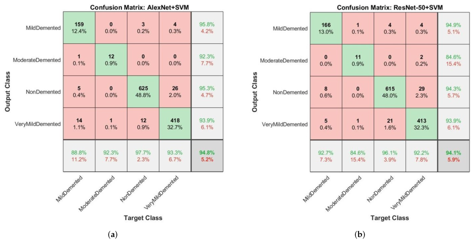
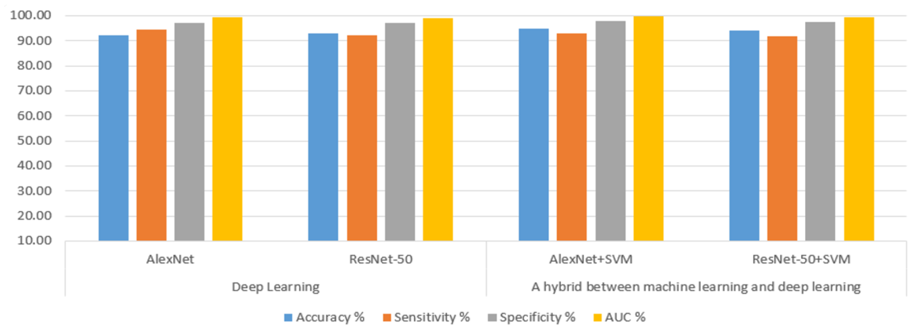
Dementia and AD are among the diseases that affect the elderly and their lives. Thus, an effective diagnosis of AD is an important factor in overcoming the disease. The volume of spending on AD and its economic impact amount to a trillion dollars. This indicates that the early diagnosis of dementia and AD is crucial. Considering the difficulty of manual diagnosis by doctors, artificial intelligence techniques have played an important role in the early diagnosis of dementia and AD. In this paper, we used two datasets. The first dataset was OASIS, which comprises medical records. SMOTE algorithm was applied to balance the dataset. The missing values were processed by replacing them using the median method. The relationship ratio between each feature and the target feature was found. The t-SNE algorithm was used to represent high-dimensional data in low-dimensional space. Finally, these features were diagnosed by four machine learning algorithms, namely, SVM, Decision Tree, Random Forest and KNN, and the dataset was divided into 80% for training and 20% for testing. All algorithms achieved effective results, the best of which was achieved by using the random forest classifier. It achieved an overall accuracy of 94% and precision, recall and F1 scores of 93%, 98% and 96%, respectively. The second dataset is MRI. All images were optimised to remove noise and artifacts through the average filter. Data augmentation method was used to balance the dataset and overcome the problem of overfitting. The dataset was divided into 80% for training and validation and 20% for testing. Deep feature maps were extracted through AlexNet and ResNet-50 models, where 9216 features were extracted for each image. Feature maps were fed to both fully connected layers. These maps were an extension of deep learning and the SVM algorithm and were the features of a hybrid method. The hybrid algorithm between machine learning and deep learning achieved better results than deep learning, with the AlexNet+SVM model achieving accuracy, sensitivity, specificity and AUC values of 94.8%, 93%, 97.75% and 99.7%, respectively.

References

1. Al-Shoukry, S.; Rassem, T.H.; Makbol, N.M. Alzheimer’s Diseases Detection by Using Deep Learning Algorithms: A Mini-Review. IEEE Access 2020, 8, 77131–77141. [Google Scholar] [CrossRef]
2. La Foresta, F.; Morabito, F.C.; Marino, S.; Dattola, S. High-density EEG signal processing based on active-source reconstruction for brain network analysis in Alzheimer’s disease. Electronics 2019, 8, 1031. [Google Scholar] [CrossRef] [Green Version]
3. Bull, F.C.; Al-Ansari, S.S.; Biddle, S.; Borodulin, K.; Buman, M.P.; Cardon, G.; Carty, C.; Chaput, J.P.; Chastin, S.; Chou, R.; et al. World Health Organization 2020 guidelines on physical activity and sedentary behaviour. Br. J. Sport Med. 2020, 54, 1451–1462. [Google Scholar] [CrossRef]
4. Xu, Z.; Deng, H.; Liu, J.; Yang, Y. Diagnosis of Alzheimer’s Disease Based on the Modified Tresnet. Electronics 2021, 10, 1908. [Google Scholar] [CrossRef]
5. Schedin-Weiss, S.; Gaunitz, S.; Sui, P.; Chen, Q.; Haslam, S.M.; Blennow, K.; Winblad, B.; Dell, A.; Tjernberg, L.O. Glycan biomarkers for Alzheimer disease correlate with T-tau and P-tau in cerebrospinal fluid in subjective cognitive impairment. FEBS J. 2020, 287, 3221–3234. [Google Scholar] [CrossRef] [Green Version]
6. Mintun, M.A.; Lo, A.C.; Duggan Evans, C.; Wessels, A.M.; Ardayfio, P.A.; Andersen, S.W.; Shcherbinin, S.; Sparks, J.; Sims, J.R.; Brys, M.; et al. Donanemab in early Alzheimer’s disease. N. Engl. J. Med. 2021, 384, 1691–1704. [Google Scholar] [CrossRef]
7. Mucke, L. Alzheimer’s disease. Nature 2009, 461, 895–897. [Google Scholar] [CrossRef] [PubMed]
8. Petersen, R.C.; Aisen, P.; Beckett, L.A.; Donohue, M.; Gamst, A.; Harvey, D.J.; Jack, C.; Jagust, W.; Shaw, L.; Toga, A.; et al. Alzheimer’s disease neuroimaging initiative (ADNI): Clinical characterization. Neurology 2010, 74, 201–209. [Google Scholar] [CrossRef] [Green Version]
9. Machado, S.D.; Tavares, J.E.D.R.; Martins, M.G.; Barbosa, J.L.V.; González, G.V.; Leithardt, V.R.Q. Ambient Intelligence Based on IoT for Assisting People with Alzheimer’s Disease Through Context Histories. Electronics 2021, 10, 1260. [Google Scholar] [CrossRef]
10. Gyanwali, B.; Lai, M.K.; Lui, B.; Liew, O.W.; Venketasubramanian, N.; Richards, A.M.; Chen, C.; Hilal, S. Blood-Based Cardiac Biomarkers and the Risk of Cognitive Decline, Cerebrovascular Disease, and Clinical Events. Stroke 2021, 52, 2275–2283. [Google Scholar] [CrossRef]
11. Mills, S.; Cain, J.; Purandare, N.; Jackson, A. Biomarkers of cerebrovascular disease in dementia. Br. J. Radiol. 2007, 80, S128–S145. [Google Scholar] [CrossRef]
12. Liu, M.; Zhang, D.; Shen, D. Relationship induced multi-template learning for diagnosis of Alzheimer’s disease and mild cognitive impairment. IEEE Trans. Med. Imaging 2016, 35, 1463–1474. [Google Scholar] [CrossRef] [Green Version]
13. Despotović, I.; Goossens, B.; Philips, W. MRI segmentation of the human brain: Challenges, methods, and applications. Comput. Math. Methods Med. 2015, 2015, 1–23. [Google Scholar] [CrossRef] [Green Version]
14. Duc, N.T.; Ryu, S.; Qureshi, M.N.I.; Choi, M.; Lee, K.H.; Lee, B. 3D-deep learning based automatic diagnosis of Alzheimer’s disease with joint MMSE prediction using resting-state fMRI. Neuroinformatics 2020, 18, 71–86. [Google Scholar] [CrossRef] [PubMed]
15. Li, H.; Habes, M.; Wolk, D.A.; Fan, Y.; Alzheimer’s Disease Neuroimaging Initiative. A deep learning model for early prediction of Alzheimer’s disease dementia based on hippocampal magnetic resonance imaging data. Alzheimer’s Dement. 2019, 15, 1059–1070. [Google Scholar] [CrossRef] [PubMed]
16. Morabito, F.C.; Campolo, M.; Mammone, N.; Versaci, M.; Franceschetti, S.; Tagliavini, F.; Sofia, V.; Fatuzzo, D.; Gambardella, A.; Labate, A.; et al. Deep learning representation from electroencephalography of early-stage Creutzfeldt-Jakob disease and features for differentiation from rapidly progressive dementia. Int. J. Neural Syst. 2017, 27, 1650039. [Google Scholar] [CrossRef]
17. Amoroso, N.; Diacono, D.; Fanizzi, A.; La Rocca, M.; Monaco, A.; Lombardi, A.; Guaragnella, C.; Bellotti, R.; Tangaro, S.; Alzheimer’s Disease Neuroimaging Initiative. Deep learning reveals Alzheimer’s disease onset in MCI subjects: Results from an international challenge. J. Neurosci. Methods 2018, 302, 3–9. [Google Scholar] [CrossRef] [Green Version]
18. Popuri, K.; Balachandar, R.; Alpert, K.; Lu, D.; Bhalla, M.; Mackenzie, I.R.; Hsiung, R.G.; Wang, L.; Beg, M.F.; Alzheimer’s Disease Neuroimaging Initiative. Development and validation of a novel dementia of Alzheimer’s type (DAT) score based on metabolism FDG-PET imaging. NeuroImage Clin. 2018, 18, 802–813. [Google Scholar] [CrossRef] [PubMed]
19. Raza, M.; Awais, M.; Ellahi, W.; Aslam, N.; Nguyen, H.X.; Le-Minh, H. Diagnosis and monitoring of Alzheimer’s patients using classical and deep learning techniques. Expert Syst. Appl. 2019, 136, 353–364. [Google Scholar] [CrossRef]
20. So, A.; Hooshyar, D.; Park, K.W.; Lim, H.S. Early diagnosis of dementia from clinical data by machine learning techniques. Appl. Sci. 2017, 7, 651. [Google Scholar] [CrossRef]
21. Chen, R.; Herskovits, E.H. Machine-learning techniques for building a diagnostic model for very mild dementia. Neuroimage 2010, 52, 234–244. [Google Scholar] [CrossRef] [PubMed] [Green Version]
22. Joshi, S.; Shenoy, P.D.; Venugopal, K.; Patnaik, L. Evaluation of different stages of dementia employing neuropsychological and machine learning techniques. In Proceedings of the 2009 First International Conference on Advanced Computing, Chennai, India, 13–15 December 2009; pp. 154–160. [Google Scholar]
23. Cho, P.C.; Chen, W.H. A double layer dementia diagnosis system using machine learning techniques. In Proceedings of the International Conference on Engineering Applications of Neural Networks, London, UK, 20–23 September 2012; pp. 402–412. [Google Scholar]
24. Trambaiolli, L.R.; Lorena, A.C.; Fraga, F.J.; Kanda, P.A.; Anghinah, R.; Nitrini, R. Improving Alzheimer’s disease diagnosis with machine learning techniques. Clin. EEG Neurosci. 2011, 42, 160–165. [Google Scholar] [CrossRef] [PubMed]
25. Shankle, W.R.; Mania, S.; Dick, M.B.; Pazzani, M.J. Simple models for estimating dementia severity using machine learning. In MEDINFO’98; IOS Press: Amsterdam, The Netherlands, 1998; pp. 472–476. [Google Scholar]
26. Yagis, E.; Citi, L.; Diciotti, S.; Marzi, C.; Atnafu, S.W.; De Herrera, A.G.S. 3D Convolutional Neural Networks for Diagnosis of Alzheimer’s Disease via Structural MRI. In Proceedings of the 2020 IEEE 33rd International Symposium on Computer-Based Medical Systems (CBMS), Rochester, MN, USA, 28–30 July 2020; pp. 65–70. [Google Scholar]
27. Pinaya, W.H.; Scarpazza, C.; Garcia-Dias, R.; Vieira, S.; Baecker, L.; F da Costa, P.; Redolfi, A.; Frisoni, G.B.; Pievani, M.; Calhoun, V.D.; et al. Using normative modelling to detect disease progression in mild cognitive impairment and Alzheimer’s disease in a cross-sectional multi-cohort study. Sci. Rep. 2021, 11, 1–13. [Google Scholar] [CrossRef]
28. Bernal-Rusiel, J.L.; Reuter, M.; Greve, D.N.; Fischl, B.; Sabuncu, M.R.; Alzheimer’s Disease Neuroimaging Initiative. Spatiotemporal linear mixed effects modeling for the mass-univariate analysis of longitudinal neuroimage data. Neuroimage 2013, 81, 358–370. [Google Scholar] [CrossRef] [Green Version]
29. Hastie, T.; Tibshirani, R.; Friedman, J. The Elements of Statistical Learnin. Cited on 2009. p. 33. Available online: http://sutlib2.sut.ac.th/sut_contents/H128492.pdf (accessed on 30 May 2021).
30. Senan, E.M.; Jadhav, M.E.; Kadam, A. Classification of PH2 Images for Early Detection of Skin Diseases. In Proceedings of the 2021 6th International Conference for Convergence in Technology (I2CT), Maharashtra, India, 2–4 April 2021; pp. 1–7. [Google Scholar]
31. Bishop, C.M. Neural Networks for Pattern Recognition; Oxford University Press: Oxford, UK, 1995. [Google Scholar]
32. Senan, E.M.; Jadhav, M.E. Techniques for the Detection of Skin Lesions in PH 2 Dermoscopy Images Using Local Binary Pattern (LBP). In Proceedings of the International Conference on Recent Trends in Image Processing and Pattern Recognition, Aurangabad, India, 3–4 January 2020; pp. 14–25. [Google Scholar]
33. Deng, L.; Yu, D. Deep learning: Methods and applications. Found. Trends Signal Process. 2014, 7, 197–387. [Google Scholar] [CrossRef] [Green Version]
34. Goodfellow, I.; Bengio, Y.; Courville, A. Deep Learning; MIT Press: Cambridge, MA, USA, 2016. [Google Scholar]
35. Bengio, Y. Learning Deep Architectures for AI; Now Publishers Inc.: Hanover, MA, USA, 2009. [Google Scholar]
36. Deng, L. A tutorial survey of architectures, algorithms, and applications for deep learning. APSIPA Trans. Signal Inf. Process. 2014, 3. [Google Scholar] [CrossRef] [Green Version]
37. Aldhyani, T.H.; Alrasheedi, M.; Alqarni, A.A.; Alzahrani, M.Y.; Bamhdi, A.M. Intelligent hybrid model to enhance time series models for predicting network traffic. IEEE Access 2020, 8, 130431–130451. [Google Scholar] [CrossRef]
38. Faust, O.; Ng, E.Y. Computer aided diagnosis for cardiovascular diseases based on ecg signals: A survey. J. Mech. Med. Biol. 2016, 16, 1640001. [Google Scholar] [CrossRef]
Figure 1. Methodology for classifying the OASIS and MRI Alzheimer’s datasets.
Electronics 10 02860 g001
Figure 2. A sample of the MRI Alzheimer’s dataset.
Electronics 10 02860 g002
Figure 3. Sample MRI images after the image enhancement process.
Electronics 10 02860 g003
Figure 4. Correlation between features of the OASIS dataset.
Electronics 10 02860 g004
Figure 5. Architecture of the AlexNet and ResNet-50 models.
Electronics 10 02860 g005
Figure 6. Confusion matrices. (a) Confusion matrix for the AlexNet to evaluate Alzheimer’s disease. (b) Confusion matrix for the ResNet-50 to evaluate Alzheimer’s disease.
Electronics 10 02860 g006
Figure 7. Confusion matrices. (a) Confusion matrix for the AlexNet-50+SVM to evaluate Alzheimer’s disease. (b) Confusion matrix for the ResNet+SVM to evaluate Alzheimer’s disease.
Electronics 10 02860 g007
Figure 8. The performances of deep learning and hybrid techniques.
Electronics 10 02860 g008