Combining Real-Time Extraction and Prediction of Musical Chord Progressions for Creative Applications

Abstract

Recently, the field of musical co-creativity has gained some momentum. In this context, our goal is twofold: to develop an intelligent listening and predictive module of chord sequences, and to propose an adapted evaluation of the associated Music Information Retrieval (MIR) tasks that are the real-time extraction of musical chord labels from a live audio stream and the prediction of a possible continuation of the extracted symbolic sequence. Indeed, this application case invites us to raise questions about the evaluation processes and methodology that are currently applied to chord-based MIR models. In this paper, we focus on musical chords since these mid-level features are frequently used to describe harmonic progressions in Western music. In the case of chords, there exists some strong inherent hierarchical and functional relationships. However, most of the research in the field of MIR focuses mainly on the performance of chord-based statistical models, without considering music-based evaluation or learning. Indeed, usual evaluations are based on a binary qualification of the classification outputs (right chord predicted versus wrong chord predicted). Therefore, we present a specifically-tailored chord analyser to measure the performances of chord-based models in terms of functional qualification of the classification outputs (by taking into account the harmonic function of the chords). Then, in order to introduce musical knowledge into the learning process for the automatic chord extraction task, we propose a specific musical distance for comparing predicted and labeled chords. Finally, we conduct investigations into the impact of including high-level metadata in chord sequence prediction learning (such as information on key or downbeat position). We show that a model can obtain better performances in terms of accuracy or perplexity, but output biased results. At the same time, a model with a lower accuracy score can output errors with more musical meaning. Therefore, performing a goal-oriented evaluation allows a better understanding of the results and a more adapted design of MIR models.

1. Introduction

The concept of musical structure can be defined as the arrangement and relations between musical elements across time. Furthermore, a piece of music possesses different levels of structure depending on the analyzed temporal scale. Indeed, elements of music such as notes (defined by their pitch, duration and timbre) can be gathered into groups like chords, motifs and phrases. Equivalently, these can be combined into larger structures such as chord progressions or choruses and verses. Thus, there can be complex and multi-scaled hierarchical and temporal relationships between different types of musical elements.

Among these different levels of music description, chords are one of the most prominent mid-level features in Western music such as pop or jazz music. The chord structure defines, at a high level of abstraction, the musical intention along the evolution of a song. Indeed, in the case of musical improvisation, it is common for musicians to agree upon a sequence of chords beforehand in order to develop an actual musical discourse along this high-level structure. Thus, a musical piece can be roughly described by its chord sequence that is commonly referred to as its harmonic structure. Some real-time music improvisation systems, such as DYCI2 [1], generate music by combining reactivity to the environment and anticipation with respect to a musical specification which can for example take the form of a chord sequence in the case we are considering. However, it would be a real improvement if the system were able to predict a continuation of the extracted sequence dynamically as a musician plays. Hence, in this paper, we focus on the extraction and prediction of musical chords sequences from a given musical signal. However, this application case invites us to raise questions about the evaluation processes and methodology that are currently applied to chord-based Music Information Retrieval (MIR) models. Indeed, we want here models that reach a high level of understanding of the underlying harmony. Therefore, the classification score that is mainly used to evaluate chord-based MIR models does not seem to be sufficient, and the use of specifically tailored evaluation process appears to be essential.

In this paper, our application goal is to combine chord extraction and chord prediction models in an intelligent listening system predicting short-term continuation of a chord sequence (architecture detailed in Section 2). The musical motivation, discussed in Section 3, comes from the field of human–machine music co-improvisation. Here, we chose to work with chord labels because chords and chord progressions are high-level abstractions that summarize the original signal without a precise level of description, but with a high level of understanding of the musician’s intent. Hence, our application case invites us to raises questions on the methodology and evaluation processes applied to MIR chord-based models. In this line of thought, we discuss in Section 4 the differences between the nature and function of chord labels, as well as the particularity of evaluation processes when chord labels are used with Machine Learning (ML) models. In order to reach our application objective, we divided the project into two main tasks: a listening module and a symbolic generation module. The listening module, presented in Section 5, extracts the musical chord structure played by the musician. Subsequently, the generative module (detailed in Section 6) predicts musical sequences based on the extracted features. In order to provide a consistent functional qualification of the classification outputs, specifically-tailored evaluation processes are carried out for both chord-based models.

2. Objectives: Extracting and Predicting Chord Progressions from a Real-Time Audio Stream

2.1. Designing a Predictive Module That Infer Chord Sequences Based on Real-Time Chord Extraction

Although musical improvisation is associated with spontaneity, it is largely based on rules and structures that allow different musicians to play together properly. In blues or jazz improvisation, these structures are usually based on fixed progression of chords that define guidelines for the whole performance, and their inference becomes very useful. Indeed, in a collective improvisation, it is essential to understand underlying musical structures. Hence, our application case is the development of a system that interacts with a musician in real time by inferring expected chord progressions.

2.2. An Intelligent Listening Module Performing Continuation of Chord Progressions

Figure 1 illustrates the general workflow of the proposed intelligent listening and predictive architecture. In this architecture, the input is an audio waveform obtained by recording a musician in real time. First, the musical signal is processed to obtain a time-frequency representation, from which we extract chord sequences. Thus, a chord label is assigned for each beat of the input signal. Finally, the prediction module receives this chord sequence and proposes a possible continuation. We also add a feedback loop in order to use the predictions to reinforce the local extraction of chords (more detailed information on the connection between the two chord-based models will be given in Section 7).

3. Musical Motivation: Inform Human–Machine Music Co-Improvisation

Our motivation lies in the field of human–machine musical co-improvisation, where the improvisation structure is generated by listening of a human musician and provides specifications to artificial musical agents. Indeed, a first autonomous creative use of the intelligent listening and predictive module could be to use a musician’s playing as input, with the interactive outputs providing chord sequences that can be improvisation guides for other musicians.

In the field of computer science applied to music, co-improvisation processes stem from the interplay between humans and computer agents. That is, a digital system able to play music coherently with a musician in real time. This leads to a co-creation process, where the human listens to the real-time output of the system, itself conditioned by the musician audio stream (see Figure 2).

A prominent example of this idea is Omax [2], which learns the specific characteristics of the musician style in real-time, and then plays along with him from this learned model. Its generative strategy (step number two in Figure 2) is based on Factor Oracle automatons [3], allowing for generating stylistically coherent music using an online or offline audio database.

In recent years, another family of software that provides musical control, while being style-sensitive has been proposed by Nika et al. [4]. In this work, the generative strategy is further improved through the concept of guidance. In this field of human–machine co-improvisation, the notion of guided music generation has two different meanings. On the one hand, guiding can be seen as a purely reactive and gradual process. This approach offers rich possibilities for interaction but cannot take advantage of prior knowledge of a temporal structure to introduce anticipatory behaviour. On the other hand, guiding can use temporal structures (named scenario) to drive the generation process of the entire musical sequence. These scenario-based systems are capable of introducing anticipatory behaviors, but require prior knowledge of the musical context (a predefined scenario).

3.1. Guiding Step-by-Step

The step-by-step process aims to produce automatic accompaniment by using purely reactive mechanisms without relying on prior knowledge. Hence, the input signal from the musician is analysed in real time and the system compares this information to its corpus, allowing for selecting the most relevant parts to generate accompaniments. For instance, SoMax [5] uses a pre-annotated corpus and extracts multimodal observations of the input musical stream in real time. Then, it retrieves the most relevant slices of music from the corpus to generate an accompaniment.

Other software such as VirtualBand [6] or Reflexive Looper [7] also rely on feature extraction (e.g., spectral centroid or chroma) to select the audio accompaniment from the database. Furthermore, improvisation software such as MASOM [8] uses specific listening modules to extract higher-features like eventfulness, pleasantness or timbre.

3.2. “Guiding” with Formal Temporal Structures

Some research projects have introduced temporal specifications to guide the process of music generation. For example, Alexandraki [9] uses a real-time listening system to perform an audio-to-score alignment and then informs an accompaniment system which concatenates pre-recorded and automatically segmented audio units. Another approach to co-improvisation is to introduce different forms of guidance as constraints for the generation of musical sequences. Indeed, constraints can be used to preserve certain structural patterns already present in the database. In this line of thought, the authors of [10] built a system to generate bagana music, a traditional Ethiopian lyre based on a first-order Markov model. A similar approach using Markov models was proposed by Eigenfeldt [11], producing corpus-based generative electronic dance music. Other research, such as that by Donze [12], applied this concept to generate monophonic solo lines similar to a given training melody based on a given chord progression.

The specification of high-level musical structures that define hard constraints on the generated sequences has been defined by Nika [4] as a musical scenario. This approach allows for defining a global orientation of the music generation process. When applied to tonal music, for instance, constraining the model with a specific temporal structure allows the generation to be directed toward a harmonic resolution (e.g., by going to the tonic).

Scenario 1.

In this work, we define a scenario as a formalized temporal structure guiding a music generation process.

An example of scenario-based systems is ImproteK [4], which uses pattern-matching algorithms on symbolic sequences. The generation process navigates a memory while matching predefined scenarios at a symbolic level. This approach is dedicated to compositional workflows as well as interactive improvisation, as the scenario can be modified via a set of pre-coded rules or with parameters controlled in real-time by an external operator.

3.3. Guiding Strategies

In 1969, Schoenberg [13] formulated a fundamental distinction between progression and succession. From their point of view, a progression is goal-oriented and future-oriented, whereas a succession only specifies a step-by-step process.

Co-improvisation systems using formal temporal structures include this notion of progression and introduce a form of anticipatory behaviour. However, the concept of scenario is limited to a predefined configuration of the system (e.g., defined before the performance), which limits the algorithm ability to predict future movements or changes within musical streams.

One idea to enrich the reactive listening would be to extract high-level structures from the musical stream in order to infer possible continuations of this structure. This model, inferring short-term scenarios for the future (e.g., chord progression), to feed a scenario-based music generation system in real time would provide anticipatory improvisations from an inferred (and not just predefined) structure.

The DYCI2 library [1] https://github.com/DYCI2/Dyci2Lib (accessed on 22 October 2021) has been developed to merge the “free”, “reactive” and “scenario-based” music generation paradigms. It proposes an adaptive temporal guidance of generative models. Based on a listening module that extracts musical features from the musician’s input or manually informed by an operator, the system will propose a scenario at each generation step. Each query is compared to previous ones and is dynamically merged, aborted and/or reordered, then launched in due time. The sound generation is then performed with a concatenative synthesis process so that the output sequences match the required short-term progression received from the listening module. Therefore, the DYCI2 library opens a promising path for the use of short-term scenarios.

Nevertheless, the short-term scenarios proposed by DYCI2 are currently generated from simple heuristics and from low-level musical features (e.g., CQT, MFCC, Chromagram). Thus, using a module that infers a short-term scenario (i.e., predicted chord sequence) from high-level feature discovery (i.e., extracted chord sequence) would be a significant improvement. Based on this inference, music generation processes could fully combine the advantages of both forms of “guidance” mentioned above.

Figure 3 illustrates the integration of our system with DYCI2. Hence, each chord sequence constitutes a “short-term scenario” for the agent, which generates a musical sequence in real time corresponding to this specification. This sequence is an “anticipation” that is stored in a buffer, waiting to unfold its rendering in due time or to be partly rewritten depending on the next scenarios sent by the listening module. At each new chord sequence received from the listening module (one per beat), the agent refines the anticipations generated in the previous step, maintaining both consistency with the future scenario, and the outputs played so far. Therefore, depending of the scenario (if the prediction at t-1 is coherent with the prediction at t (in orange on Figure 3) or not (in yellow)), DYCI2 will adapt the generation of the audio concatenated synthesis.

As a result, our goal is to provide a reactive (in the real-time sense) intelligent listening system capable of anticipating and generating improvisation from an inferred (rather than purely specified) underlying structure. In a more general perspective, our proposed intelligent listening system is a step forward for any other co-creative interaction systems [14] that seek to be in touch with live performers as well as musical knowledge in unknown (free), known (scenario), or uncertain environments (continuous scenario discovery, local scenario generation, or simply adaptive discovery of musical intentions in terms of micro-progressions).

In the next section, we raise questions about the nature and the function of chord labels. This leads to considerations that allow us to develop a specifically tailored analyser for MIR chord based models. The proposed methodology and the evaluation processes are then applied to the listening module (in Section 5) and the predictive module (in Section 6).

4. Methodology: Introducing Functional Qualification of the Classification Outputs of MIR Chord-Based Models by Taking into Account the Harmonic Function of the Chords

Deep learning methods and modern neural networks have witnessed tremendous success in Computer Vision (CV) [15] and Natural Language Processing (NLP) [16]. In the field of Music Information Retrieval (MIR), the number of published papers using Deep Learning (DL) models has also exploded in recent years and now represents the majority of the state-of-the-art models [17]. However, most of these works rely straightforwardly on successful methods that have been developed in other fields such as CV or NLP. For instance, the Convolutional Neural Networks (CNN) [18] were developed based on the observation of the mammalian visual cortex, while recurrent neural networks [19,20] and attention-based models [21,22] were first developed with a particular emphasis on language properties for NLP.

When applied to audio, these models are often used directly to classify or infer information from sequences of musical events, and have shown promising success in various applications, such as music transcription [23,24], chord estimation [25,26], orchestration [27,28], or score generation [29]. Nevertheless, DL models are often applied to music without considering its intrinsic properties. Indeed, images and time-frequency representations—and similarly scores and texts—do not share the same properties. In this perspective, chord-based MIR models could benefit from the use of musical properties in their training as well as for efficient evaluation methods.

4.1. Nature and Functions of Musical Chords

In CV, neural networks are commonly used for classification tasks, where a model is trained to identify specific objects, by providing a probability distribution over a set of predefined classes. For instance, we can train a model on a dataset containing images of ten classes of numbers. After training, this network can predict the probabilities over unseen images. Since a digit belongs to only one class, there is supposedly no ambiguity for the classification task.

In the case of music, high levels of abstraction such as chords can be associated with multiple classes. C:Maj, C:Maj7, C:Maj9 are chords of 3, 4, and 5 notes that can be considered in some contexts as labels with different levels of precision defining the same chord. Indeed, one can choose to describe a chord with a different level of detail by deleting or adding a note and, thus, changing its precise qualities. On the other hand, an ambiguity could be present if a note is only played furtively or is an anticipation of the next chord. Strong relationships exist between the different chord classes depending on the musical discourse and the hierarchical behaviour of chord labels. Hence, as underlined in recent studies [30], even expert human annotators do not agree on the precise chord estimation of an audio segment. This could be explained in part by the ambiguity of the Automatic Chord Extraction (ACE) task. On the one hand, a local extraction would define the nature of the chords, which is more related to a polyphonic pitch detection. On the other hand, one would like to transcribe the whole track by performing a functional analysis and then taking into account high-level structures. For our purpose, we prefer to consider a chord as a function that will be used for a piece of music rather than an entity that belongs solely to a specific class [13,31].

In MIR, high-level features are often associated with information that can give a musically understanding of pieces without the ability to precisely reconstruct them. For example, chords and keys can be considered as a higher level of abstraction than musical notes. In the case of the proposed intelligent listening module, the most important objective is to discover the underlying harmonic progression and not a succession of precisely annotated chords. Hence, even a wrongly predicted chord label could actually be an adequate substitute for the original chord and, therefore, still give useful information about the harmonic progression. Indeed, two chords can have different nature (for instance, C:Maj and C:Maj7) but share the same harmonic function within a chord progression.

It is important to note that these previous observations are specific to a high-level of abstraction of the musical characteristics. In the next section, we attempt to give different definitions of transcription in the field of MIR. Although only the ACE task (presented in Section 5) is directly related to automatic music transcription tasks, the sub-mentioned conclusions remain valid for the chord sequence prediction task (detailed in Section 6).

4.2. Differentiate Strict and High-Level Transcriptions in MIR

Music Information Retrieval (MIR) is a rapidly growing research field that relies on a wide variety of domains such as signal processing, psychoacoustics, computer science, machine learning, optical music recognition and all fields of music analysis and composition. In the field of MIR, automatic music transcriptions refers to several tasks that deal with different musical levels.

Klapuri [32] states that the “music transcription refers to the analysis of an acoustic musical signal so as to write down the pitch, onset time, duration, and source of each sound that occurs in it. […] Besides the common musical notation, the transcription can take many other forms, too. For example, a guitar player may find it convenient to read chord symbols which characterize the note combinations to be played in a more general manner.” In addition to this definition, Humphrey [30] describes the chord transcription task as “an abstract task related to functional analysis, taking into consideration high-level concepts such as long term musical structure, repetition, segmentation or key.” With the help of these definitions, we propose two different kinds of transcription named strict transcription and high-level transcription (see Figure 4).

Strict transcription:

We define as strict a transcription that objectively associates a unique label for each section of a musical signal. Labels are defined on the basis of a purely physical analysis and must not have any ambiguity in their definition. For example, the extraction of notes from an instrument recording is a strict transcription. There is only one set of notes that defines perfectly the recording.

High-level transcription:

We define a high-level transcription as the labelling of a musical signal into high-level musical labels. High-level musical labels include all musical information that could be subjective, such as different chords in an harmonic context, the tonality of a song, the structural division of a track, the musical genres, or any human-annotated labels based on perceptual properties.

4.3. Chord Alphabets and Functional Qualification of the Classification Outputs

By taking into account the aforementioned statements on the distinctiveness of musical data and musical chords, we detailed in this section the chord alphabets and evaluation methods tailored for the two studied MIR tasks: the chord extraction and the chord sequence continuation.

4.3.1. Definition of Chord Alphabets

There exist many qualities of musical chords (for example, maj7, min, dim) at different levels of precision. When studying a MIR task such as chord extraction or chord sequence inference, a collection of chord qualities is often defined to determine the level of precision. Thus, the chord alphabet used for this task can be increasingly complex, starting from a simple alphabet containing only major and minor chords, to one with more precisely described chords.

The chord annotations of MIR datasets [33] often include additional notes (in parentheses) and the base note (after the slash). With this notation, reference datasets have thousand chord classes with a fairly sparse distribution. For the two studied MIR tasks, we do not use these extra notes and bass notes:

$$F:maj7\left(11\right)/3\to F:maj7$$

(1)

Nevertheless, even with this first reduction, the number of chord qualities remains large, and, as detailed in Section 4.1, we consider a chord as a function that will be used for a piece of music rather than an entity that belongs solely to a specific class. Therefore, we prefer a high level of understanding of the musician’s intent instead of a precise level of description. As a result, we define three alphabets with a fixed number of chord qualities: $A_0$, $A_1$, and $A_2$. These alphabets are based on prior work on chord extraction tasks [34,35]. Figure 5 depicted the three chord alphabets used for the two MIR tasks. The number of classes in the alphabets increases gradually, chord symbols that do not fit in a particular alphabet are either reduced to the equivalent standard triad or replaced by the no chord sign $N.C.$, as indicated by the black lines.

The first alphabet $A_0$ contains all the major and minor chords, which defines a total of 25 classes:

$$A_0=\{N.C\}\cup \{P\times maj,min\}$$

(2)

where P represents the 12 pitch classes (with the assumption of equal temperament and harmonic equivalency).

Nonetheless, for example in jazz music, the standard harmonic notation includes chords that are not listed in the $A_0$ alphabet. We propose therefore an alphabet that includes all four-note chords found in major scale harmonization. This corresponds to the chord qualities and their parents annotated in the $A_1$ field in Figure 5. The no-chord class N contains other chord qualities that do not fit in a chord class, yielding a total of 73 classes:

$$A_1=\{N.C\}\cup \{P\times maj,min,dim,dim7,maj7,min7,7\}$$

(3)

Finally, the alphabet $A_2$, which is the most complete chord alphabet and that contains 14 chord qualities and 169 classes:

$$\begin{array}{c}\hfill A_2=\{N.C\}\cup \{P\times maj,min,dim,aug,maj6,min6,\\ \hfill maj7,minmaj7,min7,7,dim7,hdim7,sus2,sus4\}\end{array}$$

(4)

4.3.2. Proposed Evaluation: Functional Qualification of the Classification Outputs (by Taking into Account the Harmonic Function of the Chords)

Most of the MIR evaluations for chord-based models are binary: an extracted chord will be considered misclassified if it has a different nature than the targeted one, even if they share the same harmonic function. Hence, usual MIR evaluation methods are at odds with our needs: to have a high level of understanding of the musician’s intent, even without a precise level of description.

Motivated by the insights detailed in Section 4.1, we propose to analyse chord-based models with a functional qualification of the classification outputs. Hence, we seek to observe the qualification of what are usually considered errors. In tonal music, the harmonic functions qualify the roles and the tonal significance of chords, and the possible equivalences between them within a sequence [13,36]. Therefore, our ACE Analyzer [34] is used to analyse the results. It includes two analysis modules designed in the aim of discovering musical relationships between the chords predicted by chord-based models and the target chords. Both modules are generic, independent, and available online http://repmus.ircam.fr/dyci2/ace_analyzer (accessed on 22 October 2021).

The first module identifies errors relating to hierarchical connections or the usual rules of chord substitutions, i.e., the use of one chord in place of another in a chord progression. Some chords may have different nature (i.e., chord qualities) but have the same function within a chord progression. Therefore, a list of usual chord substitutions has been established based on musical knowledge (generally, the substituted chords have two pitches in common with the triad they replace).

The ACE Analyzer’s second module focuses on harmonic degrees. In music theory, a degree is written with a Roman character and corresponds to the position of a note inside a defined scale. The interest of using degrees is that the notation is independent of the pitch of the tonic. A degree is also assigned for each chord obtained by the harmonization of the scale, and is defined by the position of the root note inside the scale. Hence, this module calculates the harmonic degrees of the predicted chord and the target chord using the key annotations in the dataset in addition to the chords: e.g., in C, if the reduction of a chord on $A_0$ is C, it will be considered as “I”, if the reduction of a chord on $A_0$ is D:min it will be considered as “ii”, and so on. Then, it counts the harmonic degree substitutions when possible (e.g., in C, if the reduction of a chord on $A_0$ is C#, it will not correspond to any degree).

The aforementioned evaluation methods and the chord alphabets depicted in Figure 5 can be used for any chord-based MIR models.

5. Automatic Chord Extraction Tasks

In this paper, we are aiming to develop a system that interacts with a musician in real-time by inferring expected chord progressions. Hence, the two studied MIR tasks are the automatic chord extraction and the chord sequence continuation tasks. Furthermore, the insights on chord-based MIR models presented in the previous part will be applied to these two tasks.

In this section, we focus on an automatic chord extraction task which consists of extracting chord labels from an audio waveform. We propose innovative procedures that allow for introducing musical knowledge along with the training of machine learning models. Then, along with more usual evaluation (i.e., binary qualification of the classification outputs), we rely on proposed evaluation methods that take into account the qualification of the classification outputs in terms of harmonic function. These analyses are performed by applying the tailored chord evaluation presented in Section 4.3.2.

5.1. State of the Art

Due to the complexity of the chord extraction task, ACE systems are generally divided into four main modules: feature extraction, pre-filtering, pattern matching and post-filtering [37].

First, the raw signal can be pre-filtered using low-pass filters or harmonic and percussive source separation methods [38,39]. This optional step removes any noise or other percussive data that is not essential to the chord extraction objective. The audio signal is then transformed into a time-frequency representation, such as the short-time Fourier transform (STFT) or the Constant-Q transform (CQT), which yields a logarithmic frequency scale. These representations are sometimes summarized in a pitch bin vector called a chromagram [40]. Then, successive time frames of the spectral transform are averaged into context windows. This smooths the extracted features and takes into account the fact that chords are larger scale events. It was shown that this could be done effectively by feeding the STFT context windows to a CNN to obtain a clean chromagram [41].

Then, these extracted features are classified by relying on either a rule-based chord template system or a statistical model. Rule-based methods give fast results and a decent level of accuracy [42]. With these methods, the extracted features are classified using a fixed dictionary of chord profiles [43] or with a collection of decision trees [39]. However, these approaches are often sensitive to changes in the input signal’s spectral distribution and do not generalize well.

Based on a training data set in which each time frame is connected with a label, the statistical models try to uncover correlations between precomputed features and chord labels. The model is then optimized using gradient descent algorithms to determine the most appropriate parameter configuration. ACE has shown that several probabilistic models, such as the multivariate Gaussian mixture model [44] and neural networks (NN), either convolutional [25,45] or recurrent [46,47], performed well.

5.2. Proposals

We use a Convolutional Neural Network (CNN) architecture in this part because it has been shown to be a very successful statistical model for ACE tasks [35]. However, as discussed in Section 4.1, we also want to rely on the inherent relationships between musical chords to train and analyse our ACE models. Hence, we follow the procedure proposed in [34] to train a network by using prior knowledge underlying chord alphabets. Afterward, the performance of the models will be analysed with the help of the ACE analyser presented in Section 4.3.2.

5.2.1. Dataset

Our experiments are performed on the Beatles dataset as it provides the highest confidence regarding ground truth annotations [48]. This dataset consists of 180 hand-annotated songs, where each audio section is associated with a chord label. The CQT is calculated for each song using a window size of 4096 samples and a hop size of 2048. The transform is mapped to a six-octave scale with three bins per semitone, extending from C1 to C7. We augment the data by transposing everything from −6 to +6 semitones and changing the labels accordingly. Finally, we divide the data into three sets to evaluate our models: training (60 percent), validation (20 percent), and test (20 percent).

5.2.2. Models

For all the different chord alphabets, the same CNN model is trained, but adjusted with the size of the last layer to fit the chord alphabet size. On the input layer, batch normalization and Gaussian noise addition are applied. Then, three convolutional layers are followed by two fully-connected layers in the CNN architecture. The architecture is quite similar to the original chord-based CNN presented for the ACE task [25]. Dropout is introduced between each convolution layer to avoid over-fitting.

We utilize the ADAM optimizer for training, with a learning rate of $2.10-5$ and 1000 epochs. If the validation loss has not improved after 50 iterations, the learning rate is decreased. If the validation loss does not improve after 200 iterations, we end early and keep the model with the best validation accuracy. The results presented afterwards are the mean of 5-cross validation with a random split of the dataset.

5.2.3. Definition of Chord Distances

In most CNN approaches, the model does not take into account the relationships between each class when computing the loss function. In the following, this categorical distance is named $D_0$:

$$D_0(chor{d}_1,chor{d}_2)=\left\{\begin{array}{cc}0\hfill & \mathrm{if}chor{d}_1=chor{d}_2\hfill \\ 1\hfill & \mathrm{if}chor{d}_1\ne chor{d}_2\hfill \end{array}\right.$$

(5)

Here, we want to directly integrate the chord relationships in our model. For example, a C:maj is closer to a A:min than to a C#:maj. Therefore, we introduce musical distances that can be used to define the loss function.

To provide a finer description of chord label relationships, we propose two chord distances that are based on the representation of chords in either harmonic or pitch space.

5.2.4. Tonnetz Distance

A Tonnetz-space is a geometric representation of tonal space that is based on chord harmonic relationships [49,50]. We chose a Tonnetz-space generated by three transformations of the major and minor triads, each changing only one of the chords’ three notes: the relative transformation (transforms a chord into its relative major/minor), the parallel transformation (same root but major instead of minor or vice versa), and the leading-tone exchange (in a major chord, the root moves down by a semitone; in a minor chord, the fifth moves up by a semitone). The use of this space to represent chords has already yielded encouraging results for classification on the $A_0$ alphabet [51].

Here, the cost of a path between two chords is the sum of the successive transformations. Every transformation (relative, parallel and leading-tone exchange) has the same cost. In addition, if the chords have been reduced to fit the $A_0$ alphabet, an additional cost is applied. Chords that are not hierarchically connected to one of the $A_0$ chord alphabet are assigned to the No-Chord class. Thus, a cost between the chords that belongs to $A_0$ and the No-Chord class is also defined. Finally, $D_1$ is defined as the minimal distance between two chords in this space:

$$D_1(chor{d}_1,chor{d}_2)=min\left(C\right)$$

(6)

where C represents the set of all feasible path costs from $chor{d}_1$ to $chor{d}_2$ using a combination of the three transformations,

5.2.5. Euclidean Distance on Pitch Class Vectors

Pitch class vectors have been employed as an intermediate representation for ACE tasks in several studies [52]. In this paper, these pitch class profiles are used to calculate chord distances based on their harmonic content. Hence, each chord in the dictionary is assigned to a 12-dimensional binary pitch vector, with 1 indicating that the pitch is present in the chord and 0 indicating that it is not (for instance C:maj7 becomes $(1,0,0,0,1,0,0,1,0,0,0,1)$). Afterward, the Euclidean distance between two binary pitch vectors is used to define the distance between two chords:

$$D_2(chor{d}_1,chor{d}_2)=\sqrt{\sum _{i=0}^{11}{(chor{d}_1^i-chor{d}_2^i)}^2}$$

(7)

As a result, this distance accounts for the number of pitches that two chords share.

5.2.6. Introducing the Relations between Chords

In order to train the model with the proposed distances, the original labels from the Isophonics dataset http://isophonics.net/content/reference-annotations-beatles (accessed on 22 October 2021) are reduced so that they fit one of our three alphabets $A_0$, $A_1$, $A_2$. Then, we denote $y_{true}$ as the one-hot vector where each bin corresponds to a chord label in the chosen alphabet $A_i$. The model’s output, noted $y_{pred}$, is a vector of probabilities over all the chords in a given alphabet $A_i$. In the case of $D_0$, we train the model with a loss function that simply compares $y_{pred}$ to the original label $y_{true}$. However, for our proposed distances ($D_1$ and $D_2$), a similarity matrix M that associates each couple of chords to a similarity ratio is introduced:

$$M_{i,j}=\frac{1}{D_k(chor{d}_i,chor{d}_j)+K}$$

(8)

K is an arbitrary constant to avoid division by zero. The matrix M is symmetric and normalized by its maximum value to obtain $\overline{M}$. Then, $\overline{y_{true}}$ is computed and corresponds to the matrix multiplication of the old $y_{true}$ and the normalized matrix $\overline{M}$:

$$\overline{y_{true}}=y_{true}\overline{M}$$

(9)

Finally, the loss function for $D_1$ and $D_2$ is defined by a comparison between this new ground truth $\overline{y_{true}}$ and the output $y_{pred}$. Therefore, this loss function can be seen as a weighted multi-label classification.

5.3. Results

The CNN models are trained with the aforementioned chord distances and on the three chord alphabets presented in Section 4.3.1. The results are split into two parts, the first part that is the classification score of the extraction, and the second part that relies on musical rules defined in Section 4.3.2.

5.3.1. Proposed Methodology

For the ACE task, we propose to perform an evaluation based on the functional qualification of the classification outputs (i.e., by studying the harmonic function of the prediction errors). Therefore, we introduced the notion of weak or strong errors depending on the nature of the misclassified chords. Thus, using the two modules (explained in Section 4.3.2) that evaluate the results according to chord substitution rules and harmonic degrees will help to evaluate the ACE models by using a functional approach. For our experiments, we first evaluate models with the usual evaluation (a binary qualification of the classification outputs); then, we perform our proposed analysis in order to understand the functional qualification of the errors for the different models.

5.3.2. Usual Evaluation Binary Qualification of the Classification Outputs (Right Chord Predicted vs. Wrong Chord Predicted)

In order to compare the results with other ACE models, the models are evaluated on three MIREX alphabets: Major/Minor, Sevenths, and Tetrads. [53]. These alphabets correspond roughly to three alphabets defined in Section 4.3.1 (Major/Minor ∼$A_0$, Sevenths ∼$A_1$, Tetrads ∼$A_2$).

CNN models that have the same architecture are trained with varying chord distances ($D_0$, $D_1$ and $D_2$) and an initial chord reduction on different alphabets ($A_0$, $A_1$ and $A_2$). Then, the models are evaluated with the help of the MIREX evaluation library mir_eval https://craffel.github.io/mir_eval/ (accessed on 22 October 2021) on the three selected MIREX alphabets.

According to the results of

Table 1. Results of the 5-fold with the standard deviation: evaluation on MIREX Maj/Min (∼reduction on $A_0$), MIREX Sevenths (∼reduction on $A_1$) and MIREX Tetrads (∼reduction on $A_2$).

Model	MIREX Maj/Min	MIREX Sevenths	MIREX Tetrads
$A_0$-$D_0$	74.97 ± 1.20	_	_
$A_0$-$D_1$	75.39 ± 1.55	_	_
$A_0$-$D_2$	75.22 ± 2.15	_	_
$A_1$-$D_0$	74.30 ± 1.22	63.26 ± 3.09	_
$A_1$-$D_1$	75.86 ± 1.11	62.38 ± 3.00	_
$A_1$-$D_2$	75.47 ± 2.16	63.96 ± 3.87	_
$A_2$-$D_0$	74.86 ± 0.94	63.63 ± 3.53	63.62 ± 3.53
$A_2$-$D_1$	76.00 ± 1.63	61.11 ± 3.86	61.14 ± 3.84
$A_2$-$D_2$	75.29 ± 2.02	64.32 ± 3.62	64.38 ± 3.61

, even if the classification score is very close between models, it appears to better to utilize a distance that takes into consideration the musical relationships between chords when using the Major/Minor alphabet. However, for more complex chord alphabets, the Tonnetz-based distance ($D_1$) applies a penalty of reduction to the $A_0$ alphabet. Hence, this distance seems not suited for more complex chords alphabets, at least in terms of classification score. On the other hand, the Euclidean distance between pitch vectors ($D_2$) always obtains a better classification score on every chord alphabet.

Nonetheless, the MIREX evaluation uses a binary score to compare chords. Because of this approach, the qualities of the classification errors cannot be evaluated. Indeed, for our application case, one could prefer an ACE model with a similar accuracy score but with a better understanding of the underlying harmony.

5.3.3. Proposed Evaluation: Functional Qualification of the Classification Outputs (by Taking into Account the Harmonic Function of the Chords)

In the following experiments, we rely on our specially designed ACE analyser to understand the performance of each model by examining their errors. Our main hypothesis is that, in a real use case, a model can have a similar classification accuracy score but produce errors that have strong musical significance. Indeed, chords have strong inherent hierarchical and functional relationships. For example, misclassifying a C:Maj into A:min or C#:Maj will be seen as equally incorrect under standard evaluation criteria. However, C:Maj and A:min are relative chords, but C:Maj and C#:Maj belong to very different sets of keys. Thus, if the harmonic function is preserved, a misclassified chord can be accepted from a musical point of view and we call this a weak error. Therefore, in the following, we measure the performance of the models, which includes its propensity to output weak errors instead of strong errors (i.e., errors that are not musically accepted).

Substitution Rules

Table 2. Left: total percentage of errors corresponding to inclusions or chord substitution rules, right: percentage of errors with inclusion in the correct triad (% of the total number of errors).

Model	Tot.	⊂ Maj	⊂ min
$A_0$-$D_0$	34.93	_	_
$A_0$-$D_1$	36.12	_	_
$A_0$-$D_2$	35.37	_	_
$A_1$-$D_0$	52.40	23.82	4.37
$A_1$-$D_1$	57.67	28.31	5.37
$A_1$-$D_2$	55.17	25.70	4.21
$A_2$-$D_0$	55.28	26.51	4.29
$A_2$-$D_1$	60.47	31.61	6.16
$A_2$-$D_2$	55.45	25.74	4.78

presents: Tot., the total fraction of errors that can be explained by the whole set of substitution rules implemented in the ACE analyser (see Section 4.3.2), and ⊂ Maj and ⊂ min, the errors with inclusions in the correct triad (e.g., C:maj instead of C:maj7, C:min7 instead of C:min).

Table 3. Left: percentage of errors corresponding to usual chords substitutions rules, right: percentage of errors “major instead of minor” or inversely (% of the total number of errors).

Model	rel. M	rel. m	T subs. 2	m→M	M→m
$A_0$-$D_0$	4.19	5.15	2.37	7.26	12.9
$A_0$-$D_1$	4.40	5.20	2.47	7.66	13.4
$A_0$-$D_2$	5.13	4.87	2.26	8.89	10.89
$A_1$-$D_0$	2.63	3.93	1.53	4.46	8.83
$A_1$-$D_1$	3.05	3.36	1.58	5.53	7.52
$A_1$-$D_2$	3.02	4.00	1.62	5.84	8.07
$A_2$-$D_0$	2.54	4.15	1.51	4.96	8.54
$A_2$-$D_1$	2.79	2.97	1.54	5.29	7.46
$A_2$-$D_2$	3.11	4.26	1.63	5.34	7.59

presents the percentages of errors corresponding to widely used substitution rules: rel. m and rel. M, relative minor and major; T subs. 2, tonic substitution different from rel. m or rel. M (e.g., E:min7 instead or C:maj7), and the percentages of errors m→M and M→m, same root but major instead of minor (or inversely) after reduction to triad. The tables only show the categories representing more than $1\%$ of the total number of errors, but other substitutions (that will not be discussed here) were analysed: tritone substitution, substitute dominant, and equivalence of some dim7 chords modulo inversions.

First, Tot. in Table 2 shows that a huge fraction of errors can be explained by usual substitution rules. This percentage can reach 60.47 percent, implying that many classification errors provide useful indications since they associate chords with equivalent harmonic function. For example, Table 3 reveals that relative major/minor substitutions account for a considerable portion of errors (up to 10%). Furthermore, the percentage in Tot. (Table 2) increases with the size of the alphabet for the three distances: larger alphabets imply more errors that preserve the harmonic function.

Second, for $A_0$, $A_1$ and $A_2$, using $D_1$ instead of $D_0$ increases the fraction of errors attributed to categories in Table 3 (and in almost all the configurations when using $D_2$). Since all of these operations are normally considered as valid chord substitutions, this shows an improvement in the ratio of the right harmonic function to the wrong harmonic function, i.e., in the ratio of weak to strong errors. Finally, results indicate that a significant number of errors (between 28.19 percent and 37.77 percent) for $A_1$ and $A_2$ correspond to inclusions in major or minor chords (⊂ Maj and ⊂ min, Table 2). Therefore, these classifications can be considered as correct from a functional perspective.

Harmonic Degrees

The results of the second module of the analyser reported in Section 4.3.2 are analyzed in this section. As seen in

Table 4. Errors occurring when the target is non-diatonic (% of the total number of errors), non-diatonic prediction errors (% of the errors on diatonic targets).

Model	Non-Diat. Targ.	Non-Diat. Pred.
$A_0$-$D_0$	37.96	28.41
$A_0$-$D_1$	44.39	15.82
$A_0$-$D_2$	45.87	17.60
$A_1$-$D_0$	38.05	21.26
$A_1$-$D_1$	37.94	20.63
$A_1$-$D_2$	38.77	20.23
$A_2$-$D_0$	37.13	30.01
$A_2$-$D_1$	36.99	28.41
$A_2$-$D_2$	37.96	28.24

, the module first determines whether the target chord is diatonic (i.e., belongs to the harmony of the key).

If it is the case, the notion of incorrect degree for the predicted chord is relevant, and the percentage of errors corresponding to substitutions of degrees is computed (see

Table 5. Errors (>2%) corresponding to degrees substitutions (% of the total number of errors on diatonic targets). In this table, columns I∼IV correspond to totals of the errors that satisfy: I substituted to IV or IV substituted to I.

Model	I∼IV	I∼V	IV∼V	I∼vi	IV∼ii	I∼iii
$A_0$-$D_0$	17.41	14.04	4.54	4.22	5.41	2.13
$A_0$-$D_1$	17.02	13.67	3.33	4.08	6.51	3.49
$A_0$-$D_2$	16.16	13.60	3.08	5.65	6.25	3.66
$A_1$-$D_0$	17.53	13.72	3.67	5.25	4.65	3.5
$A_1$-$D_1$	15.88	13.82	3.48	4.95	6.26	3.46
$A_1$-$D_2$	16.73	13.45	3.36	4.70	5.75	2.97
$A_2$-$D_0$	16.90	13.51	3.68	4.45	5.06	3.32
$A_2$-$D_1$	16.81	13.60	3.85	4.57	5.37	3.59
$A_2$-$D_2$	16.78	12.96	3.84	5.19	7.01	3.45

).

The first interesting fact revealed by Table 4 is that 37.99% to 45.87% of the errors occur when the target chord is non-diatonic. It also demonstrates that using $D_1$ or $D_2$ instead of $D_0$ reduces the fraction of errors corresponding to non-diatonic predicted chords (Table 4, particularly $A_0$), which means that the errors are more likely to stay in the right key.

In Table 5, high percentages of errors are associated with errors I∼V (up to 14.04%), I∼IV (up to 17.41%), or IV∼V (up to 4.54%). These errors are not usual substitutions, and IV∼V and I∼IV have respectively 0 and 1 pitch in common. In most circumstances, these percentages tend to decrease on alphabets $A_1$ or $A_2$ and when using more musical distances (particularly $D_2$). Conversely, it increases the amount of errors in the right part of Table 5 containing usual substitutions: once again, the more precise the musical representation is, the more correct the harmonic functions tend to be.

5.4. Conclusions

In an attempt to bridge the gap between musically-informed and statistical models in the ACE field, we experimented the training of Deep Learning based models with the help of musical distances reflecting the relationships between chords. To do so, we trained CNN models on different chord alphabets and with different distances. In order to evaluate our models with a musically oriented approach, we relied on a specifically tailored ACE analyser. We concluded that training the models using distances reflecting the relationships between chords (e.g., within a Tonnetz-space or with pitch class profiles) improves the results both in terms of classification scores and in terms of harmonic functions.

6. Chord Sequence Continuation Tasks

The goal of this article is to propose a system that interacts with a musician in real time by inferring expected chord progressions. In the previous part, we focused on the automatic chord extraction module. This section will present studies on the chord sequence continuation model.

From a technical point of view, our aim is to predict the eight next beat-wise chords given eight beat-wise chords. The eight beat-wise chords that will be given to the model are those extracted with the ACE model. However, for the training of the chord sequence inference model, we will rely on datasets that are only made of symbolic chord progressions. The combination on the two systems will be detailed further in Section 7.

For this task of automatic chord sequence continuation, it has been proven that using additional musical high-level information, such as the key or the downbeat position, within the learning of machine learning models would improve chord sequence continuations in terms of accuracy score. Nevertheless, studying the impact on the predictions in terms of the functional qualification of the classification outputs (by taking into account the harmonic function of the chords) is still an open question. Therefore, in this section, the impact of using additional high-level musical information for the task of chord sequence inference is also studied in terms of qualification of the errors.

6.1. State of the Art

Most recent works on symbolic music inference and symbolic music continuation rely on machine learning and probabilistic models to infer musical information from a dataset of examples. Indeed, neural networks have shown promising results in the generation of new musical material from scratch or as the continuation of a track composed by a human [27,29]. However, these works operate at the note level, and not at the level of chords or chord progressions. In the field of chord sequence continuation or chord sequence generation, most works aim to infer the chord transition probabilities without accounting for the duration of each chord. This research often entails Hidden Markov Models (HMMs) and N-Gram models [54,55,56]. Nevertheless, sophisticated ACE models use a combination of statistical models in order to extract chords along with other musical information such as the track segmentation [57], the chord duration [58], the downbeat position [59] or the key estimation [60]. Depending on the temporal granularity, a lot of inference model use in ACE acts as a temporal smoothing system and gives a very high probability in the self-transition of chords [47,58]. Indeed, it has been shown that the highest predictive score is obtained by a simple identity function in performing continuation with short time frames [28].

Relying on a beat-level quantification appears as a reasonable temporal scale for studying chord transitions. At this time scale, promising results have already been obtained with Long Short-Term Memory (LSTM) networks [61] for generating beat-wise chord sequences matching a monophonic melody. More recent research has focused on the continuation of a beat-wise chord sequence using LSTM [62]. In this work, the aforementioned problem of large self-transition rates is partly alleviated by introducing a temperature factor that modifies the output distribution. At each step of the generation, this mechanism penalizes the self-transition in the generated chord sequence. More generally, it has been repeatedly observed that using LSTM for chord sequence continuation can propagate errors along the prediction [63]. Using teacher forcing allows for minimising this error propagation by feeding ground-truth during the training of the network [64]. However, even with this kind of training, a feed-forward model composed by simple stacks of Multi-Layer Perceptron (MLP) can outperform LSTM for chord sequence continuation [65].

6.2. Proposals

The information on key is highly correlated to the nature of chords that will be present in a song. For each key (minor or major), we have a specific set of musical notes called the scale. In addition, the downbeat position is defined as the first beat of a measure. Depending on its time signature, a measure is often composed by four beats. It has been shown that that beat-wise chords tend to be repeated intensively and that any structural information could give useful information on the chord transitions [59,65].

Using additional musical information such as the chord duration [66] or the information on downbeat position [67] has already shown an improvement in terms of perplexity or mean information content for the task of chord sequence prediction. Nevertheless, understanding the musical impact of using such high-level musical information for the inference of chord sequences is still an understudied area that we explore here through the use of musical relationships between targeted and predicted chords.

In this section, the impact of using high-level musical information for the continuation of chord sequences is studied through a functional qualification of the classification outputs. In this study, we propose to train several models for the prediction of the eight next beat-wise chords given eight beat-wise chords.

The inputs for baseline models are only the initial chord sequence. However, in order to study the impact of adding extra information for the continuation of chord sequences, we add two other pieces of musical information as input: the information on downbeat position and key. Then, we evaluate the impact of using additional high-level information for this task with the help of the specifically tailored chord analyser presented in Section 4.3.2.

6.2.1. Dataset

The Realbook dataset [62] is used for the training of chord sequence continuation models. It contains 2846 jazz songs based on band-in-a-box files http://bhs.minor9.com/ (accessed on 22 October 2021). All files come in a xlab format and contain time-aligned beat and chord information. In order to work at the beat level, the xlab files are processed to obtain a sequence of one chord per beat for each song. Our tests are made on three different alphabet reductions: $A_0$, $A_1$ and $A_2$ (detailed in Section 4.3.1). Then, 5-fold cross-validation is performed by randomly splitting the song files into training (0.8), validation (0.1), and test (0.1) sets with five different random seeds for the splits (the statistics reported in the following correspond to the average of the resulting five scores). Since we do not want a model that predicts exactly the input chord sequence, we propose to remove from the dataset all files that contain the same $A_2$ chord (see Figure 5) repeated for more than eight bars, leading to a total of 78 discarded songs. For all the remaining songs, the beginning of the song is padded with seven beat-wise $N.C$ symbols and we use all chord sub-sequences that contain 16 beat aligned chords, ending where the target is the last eight chords of each song.

6.2.2. Key and Downbeat as Inputs

The inputs for baseline models are only a sequence of eight beat-wise chords. However, we propose to give the information on key or downbeat position as input of our neural networks along with the initial chord sequence.

In diatonic music, the key defines a scale or a series of notes. Considering the major and the natural minor keys for each of the 12 possible tonics plus the No-key symbol, we obtain an alphabet of 25 elements, where P represents the 12 pitch classes and N is the No-key symbol:

$$D_{key}=\left\{N\right\}\cup \{P\times maj,min\}$$

(10)

Chord changes are strongly correlated with rhythmic structure and the downbeat position. The downbeat position is defined as the first beat of each bar. In this work, the information on downbeat position is introduced during the learning by numerating each beat in each measure of the input chord sequence. We note that, in our training dataset, the majority of the tracks have a binary metric (often 4/4). Then, the downbeat position information of each chord in the predicted sequence is a value between 1 and 4.

For our learning task, all the musical information (chord, key and downbeat position) are encoded through a one-hot vector that has the size of the corresponding alphabet.

Thus, in the baseline model called the MLP-Vanilla, the inputs of the models are only the initial sequences of eight chords (see Figure 6, input a). In order to study the impact of adding extra information for the continuation of chord sequences, we add two other pieces of musical information available in the proposed dataset. For MLP-Key, the inputs of our model is the initial chord sequence and the key (Figure 6 part a and b). For MLP-Beat, we use the downbeat position but not the key (Figure 6 part a and c). Finally, for MLP-KeyBeat, we use both key and downbeat position as inputs (Figure 6 part a, b and c). The architecture of these three models is similar to the MLP-Vanilla, except for the first layers that will be shaped to fit the size of the inputs.

6.2.3. Learning the Information on Key and Downbeat Position

Instead of using the ground-truth information such as for MLP-K and MLP-B, we propose in a preliminary experiment to train a network to recognize the key or the downbeat position of an input chord sequence. In the following, this model is named MLP-Aug.

Hence, in order to perform the training of our model, the complete loss is defined as the sum of the prediction loss related to the accurateness of the chord sequence continuation, and the additional losses ${\mathcal{L}}_{downbeat}$ for downbeat and ${\mathcal{L}}_{key}$ for key detection:

$${\mathcal{L}}_{total}={\lambda }_p{\mathcal{L}}_{prediction}+{\mathcal{L}}_{downbeat}+{\mathcal{L}}_{key}$$

(11)

We first train our models to improve the prediction of the downbeat and the key, by setting ${\lambda }_p=0$. Thus, we freeze the two sub-networks and train the network by introducing the prediction loss on the chord sequence. The overall architecture is depicted in Figure 7.

Therefore, we observe in

Table 6. Mean prediction accuracy and standard deviation on the 5-fold for the learning of the key and the downbeat information on $A_0$, $A_1$ and $A_2$ (prediction performed on a symbolic sequence of eight chords).

	${\mathit{A}}_0$	${\mathit{A}}_1$	${\mathit{A}}_2$
Key	53.57 ± 1.73	59.89 ± 3.35	61.12 ± 1.97
Downbeat	88.15 ± 0.60	89.56 ± 0.75	89.76 ± 0.82

that, when the chord alphabet comes with more classes, it increases the prediction accuracy for the key and the downbeat position. Indeed, adding chords with enriched notes will obviously help the network to recognize the key. Some of these chords could also be passing chords and will be located at specific positions within the bar, helping the network to determine the downbeat position.

6.3. Models and Training

In order to evaluate the proposed models, we compare them to several state-of-the-art methods for chord sequence continuation. In this section, we briefly introduce these models and the different parameters used for these experiments.

6.3.1. Naive Baselines

We consider one naive baseline: a repetition model that repeats the last chord of the input sequence.

6.3.2. N-Grams

A N-gram model is trained using the Kneser–Ney smoothing algorithm [68], with $N=9$. This model estimates the prediction probability of the following chord given an input sequence of the previous $N-1$ chords. Unlike neural network models, we do not pad the dataset with N.C. symbols at the beginning of each song. Furthermore, as this method does not need a validation set, we merge the train and validation set and evaluate our model on the test set. During the decoding phase, we use a beam search, saving only the top 100 states (each state contains a sequence of nine chords with their associated probabilities) at each step. The final transition probability of a chord for each step is calculated as the sum of the normalized probabilities of each state in the beam.

6.3.3. MLP-Vanilla

An encoder–decoder architecture is used for the vanilla MLP. The inputs that correspond to a sequence of eight chords are flattened to one vector and a two-dimensional softmax if used on the output in order to apply a Temporal Cross-Entropy loss (see Equation (12)) between the prediction and the target. A batch normalization and a dropout of 0.6 are applied between each layer of the network. In this task, the use of a bottleneck between the encoder and the decoder slightly improved the results compared to the classical MLP. All encoder and decoder blocks are defined as fully-connected layers with ReLU activation. We performed a grid search to select the most adapted network with a variation on four different parameters: the number of layers ($nb\_l\in [1,2,3]$), the size of the hidden layers ($nb\_h\in [100,200,500,1000]$), the size of the bottleneck ($nb\_bn\in [10,20,50,100]$), and the dropout ratio ($r\_do\in [0,0.2,0.4,0.6,0.8]$). Some of these parameters are depicted in Figure 8.

Regarding the accuracy scores and the number of parameters of these models, the MLP-Van that we selected is defined by $[nb\_l=1;nb\_h=500;nb\_bn=50,r\_do=0.4].$

6.3.4. LSTM

A sequence to sequence architecture is used to build our model [69]. Thus, the proposed network is divided into two parts (an encoder and a decoder). The encoder extracts useful information of the input sequences and gives this hidden representation to the decoder, which generates the output sequence. The encoder transforms the input chord sequence into a latent representation that will be fed to the decoder at each step. We propose to introduce a bottleneck to compress the latent variable between the encoder and the decoder. In addition, an attention mechanism is used for the decoder [70]. Thus, the decoder generates the prediction for the next chords for each step of the predicted continuation sequence. This process of generating the chords of the predicted sequence in an iterative way by using LSTM units has been described in previous papers such as with the Seq2Seq model [69]. In order to mitigate the problem of the decoder error propagating across time steps of the prediction, we train our model with the teacher forcing algorithm [64]. Thus, the decoder uses randomly the ground-truth label instead of his own preceding prediction for the sequence continuation. We decrease the teacher forcing ratio from $0.5$ to 0 along the training. Once again, we did a grid search to find correct model parameters. Regarding the accuracy scores and the number of parameters of these models, the LSTM that we selected has a bottleneck and is defined by $[nb\_l=1;nb\_h=200;nb\_bn=50,r\_do=0.4].$

6.3.5. MLP-MS

A multi-scale model which predicts the next eight chords directly, eliminating the error propagation issue which inherently exists in single-step continuation models. It provides a multi-scale modeling of chord progressions at different levels of granularity by introducing an aggregation approach, summarizing input chords at different time scales. This multi-scale design allows the model to capture the higher-level structure of chord sequences, even in the presence of multiple repeated chords [65].

6.3.6. Training Procedure

Our neural network models are trained with the ADAM optimizer with a decreasing learning rate starting at ${10}^{-3}$ and divided by a factor of two when the validation accuracy does not decrease for 10 epochs. We follow a 5-fold cross-validation training procedure, by randomly splitting the dataset into train (0.8), valid (0.1) and test (0.1) sets. In order to evaluate the efficiency of our proposed methods, we also train state-of-the-art baseline models for chord sequence continuation described in the previous part.

Chord Sequence Continuation Loss

For the task of chord sequence continuation, our neural network models are trained with the help of a temporal cross entropy loss. For each chord in the predicted sequence, we apply a Cross Entropy (CE) loss between the target chord and the predicted chord in this position:

$${\mathcal{L}}_{prediction}=\sum _{t=0}^{T}CE\left(pred\left(t\right),target\left(t\right)\right)$$

(12)

Thus, $L_{prediction}$ is the sum of the CE for each time-step of the chord sequence continuation (in the following experiments, the continuation is a sequence of eight beat-wise chords).

6.4. Results

The use of specifically tailored analysers allows a better understanding of the impact of using additional high-level musical information. Indeed, the functional qualification of the classification outputs is primordial in order to analyze the results beyond the classification score and understand in which musical ways the information on key or on the downbeat position can affect the prediction of the different models.

6.4.1. Proposed Methodology

In this paper, we propose to evaluate chord-based models with the help of our specifically tailored analyser that integrate relationships between predicted and targeted chords. Indeed, the classification accuracy score that is used commonly for these kinds of MIR tasks does not provide an in-depth understanding on the performance of the models. Hence, in the following, we are interested in the measurement of performance of the models, which includes its propensity to output weak errors (accepted from a musical point of view) instead of strong errors (errors that are not musically accepted). Therefore, we rely on our ACE analyser to perform musically oriented tests of the classification errors.

In the following, the evolution of the predictive accuracy score is first compared on the different chord alphabet for all the different configurations. Then, complementary predictive evaluations are performed by dividing the dataset between diatonic chords, which are built upon notes of the scale defined by the key of the track and non-diatonic chords. The division of chords into two subsets allows us to see more precisely the impact of the use of musical information. We observe that the use of the key or the position of the downbeat as input strongly constrains the network during the inference of the continuation of a chord sequence. This encourages one to consider the evaluation of the results in adequacy with the applicative purpose. Indeed, this work shows that it would not be relevant to use the same metric when the objective is to obtain an accurate transcription or a functional harmonic information. In the latter case, in the context of the development of a listening module for human musical improvisation machine, we suggest to rely on a more musically-informed evaluation. In order to complete this study, we rely on the ACE analyser (presented in Section 4.3.2) in order to determine the harmonic functions of the predicted and targeted chords. Indeed, the use of this specific analyser allows a better musical understanding of the models’ output than a classification score. Once again, the dataset is divided into diatonic and non-diatonic chords. Thereafter, the ACE analyser is used independently on both subsets in order to understand in depth the differences between the proposed models.

6.4.2. General Predictive Accuracy

Our first experiment is the evaluation of the different models on the three alphabets $A_0$, $A_1$ and $A_2$. We compute the mean prediction accuracy over the output chord sequence (see

Table 7. Mean prediction accuracy and the standard deviation for each method over the chord alphabets $A_0$, $A_1$ and $A_2$ on the 5-fold.

Model	${\mathit{A}}_0$	${\mathit{A}}_1$	${\mathit{A}}_2$
Repeat	32.68 ± 0.75	29.86 ± 0.46	29.37 ± 0.52
9-Gram	37.87 ± 0.64	34.45 ± 0.65	33.76 ± 0.53
LSTM	40.82 ± 0.63	37.22 ± 0.44	35.29 ± 0.43
MLP-Van	41.49 ± 0.63	37.04 ± 0.40	35.47 ± 0.62
MLP-MS	41.45 ± 0.70	37.32 ± 0.32	35.91 ± 0.52
MLP-K	43.85 ± 0.62	37.72 ± 0.32	36.06 ± 0.57
MLP-B	42.06 ± 0.61	38.15 ± 0.37	36.65 ± 0.55
MLP-KB	44.86 ± 0.66	39.33 ± 0.23	37.87 ± 0.70
MLP-Aug	41.38 ± 0.72	37.50 ± 0.33	36.10 ± 0.56

). As a baseline, we present on the first line the predictive score for the repeat model. We note that these models obtain a rather high accuracy even for the most complex alphabets. This can be explained by the fact that it is not rare for chords to be played more than one single beat.

For all the models, we observe that the accuracy decreases when using more complex chord alphabets. With the binary qualification of the classification outputs, we see that the introductions of key and/or downbeat position improve the accuracy score of the MLP on every alphabet, and that the highest accuracy is reached when both are introduced in the MLP model. The MLP-MS models show globally an improvement compared to MLP-Van models. The model that also learns the information on key and downbeat position, denoted MLP-Aug, shows better accuracy scores than MLP-Van or MLP-MS. We also observe that 9-Gram and LSTM models offer similar or worse results in terms of mean prediction accuracy score compared to the MLP models. In order to study the impact of using additional musical information in terms of functional qualifications of the classification outputs, the following section focuses only on the MLP models.

6.4.3. Behind the Score: Understanding the Errors

In this section, we propose to analyze the chord sequence predictions through a functional qualification of the classification outputs (by taking into account the harmonic function of the chords). As aforementioned, the key of a track defines a musical scale, and diatonic chords are build upon this set of notes. Thus, in this section, we first study the evolution of the prediction score when splitting the dataset between diatonic and non-diatonic chords.

Thereafter, we compare the functional relationships between the predicted and the targeted chords. Our goal is twofold: to understand what causes the errors in the first place, and to distinguish “weak” from “strong” errors with a functional approach. As detailed in Section 4.1, the harmonic functions qualify the roles and the tonal significances of chords, and the possible equivalences between them within a sequence [13,36]. To perform these analyses, we use the ACE Analyzer library (see Section 4.3.2) that includes two modules discovering some formal musical relationships between the target chords and the predicted chords.

Distinguishing between Diatonic and Non-Diatonic Targets

For the first experiment, we divide our dataset into diatonic chords and non-diatonic chords. As aforementioned, the key of a track defines a musical scale, and diatonic chords are the ones built upon this set of notes.

Table 8. Mean prediction accuracy for each method over the different chord alphabets on diatonic (D.) and non-diatonic (N-D.) chord targets. The amounts of associated items in the test dataset are in parentheses.

Alphabet	${\mathit{A}}_0$		${\mathit{A}}_1$		${\mathit{A}}_2$
Chord tgt.	D. (1.44M)	N-D. (490k)	D. (1.37M)	N-D. (559k)	D. (1.33M)	N-D. (602k)
MLP-Van	45.88 (660k)	28.58 (139k)	41.96 (574k)	24.98 (139k)	40.80 (541k)	23.70 (142k)
MLP-MS	45.78 (659k)	28.73 (140k)	42.27 (579k)	25.20 (140k)	41.25 (547k)	24.10 (145k)
MLP-K	50.53 (727k)	24.21 (118k)	44.29 (606k)	21.63 (121k)	42.95 (570k)	20.83 (125k)
MLP-B	46.44 (668k)	29.21 (143k)	43.11 (590k)	25.99 (145k)	42.08 (558k)	24.63 (148k)
MLP-KB	51.48 (741k)	25.39 (124k)	45.89 (628k)	23.26 (130k)	44.95 (596k)	22.22 (133k)
MLP-Aug	45.91 (660k)	28.05 (137k)	42.55 (582k)	25.14 (140k)	41.68 (553k)	23.78 (143k)

shows the accuracy scores and the number of correct predictions depending on the nature of the targeted chords for the different models over the different alphabets.

We observe that adding information on the downbeat position (MLP-Beat) improves the prediction scores for both diatonic and non-diatonic chords. The model taking the key into account (MLP-Key) shows an important improvement for the diatonic chords; nevertheless, we observe a decrease of the classification score for the non-diatonic targets. Finally, the model using both key and downbeat position (MLP-KB) presents a better score for the diatonic targets but loses accuracy on the non-diatonic targets. Even if the classification scores of MLP-KB are slightly better for every chord alphabet compared to MLP-Key, we note that the classification score for the non-diatonic targets is better if we do not take the key into account. The model that learns information on key and downbeat, MLP-Aug, obtains better results than MLP-Van on every alphabet for diatonic and non-diatonic chord targets. Thus, learning the key instead of using it does not decrease the accuracy score for the non-diatonic chord targets.

These first observations lead to the conclusion that the use of high-level musical information could be envisaged in different ways depending on the framework in which chord prediction is realised, as well as on the repertoire and the corpus used. For example, in the context of popular music, the accuracy of diatonic chords could be privileged. Therefore, this would encourage the use of the information on key in this situation. Conversely, in a jazz context where modulations, borrowing chords from other keys, and chromatisms are more frequent, one could prefer to gain in precision on non-diatonic chords thanks to the information on downbeat position only, even if it means losing some accuracy on diatonic chords. This conclusion is strengthened if, as studied below, the loss in accuracy is compensated by an improvement in the ratio of classification errors providing nevertheless right harmonic functions.

Substitution Rules and Functional Equivalences

Here, we evaluate models based on the harmonic function of each chord by using relationships between the predicted and the targeted chords. We first study the errors corresponding to usual chord substitutions rules: using a chord in place of another within a chord progression (usually, substituted chords have two pitches in common with the triad that they are replacing); and hierarchical relationships: prediction errors included in the correct triads (e.g., C:maj instead of C:maj7, C:min7 instead of C:min).

In

Table 9. Percentage of errors corresponding to inclusions or usual chord substitution rules.

Model	⊂ Maj	⊂ min	rel.M	rel.m	T s.2
$A_0$-MLP-Van	_	_	4.14	1.64	1.14
$A_0$-MLP-MS	_	_	4.14	1.68	1.17
$A_0$-MLP-K	_	_	4.49	1.72	1.17
$A_0$-MLP-B	_	_	4.33	1.62	1.12
$A_0$-MLP-KB	_	_	4.67	1.69	1.12
$A_0$-MLP-Aug	_	_	4.18	1.61	1.12
$A_1$-MLP-Van	6.96	0.98	3.52	1.58	1.32
$A_1$-MLP-MS	7.07	1.02	3.44	1.68	1.31
$A_1$-MLP-K	7.04	1.12	3.58	1.62	1.29
$A_1$-MLP-B	7.45	1.07	3.58	1.57	1.25
$A_1$-MLP-KB	7.46	1.17	3.72	1.68	1.29
$A_1$-MLP-Aug	7.22	1.06	3.47	1.68	1.32
$A_2$-MLP-Van	7.69	1.14	3.34	1.61	1.23
$A_2$-MLP-MS	7.72	1.19	3.30	1.71	1.29
$A_2$-MLP-K	7.88	1.25	3.42	1.64	1.30
$A_2$-MLP-B	8.30	1.19	3.42	1.68	1.20
$A_2$-MLP-KB	8.40	1.36	3.53	1.67	1.29
$A_2$-MLP-Aug	7.96	1.17	3.27	1.76	1.29

, we present the percentage of errors explained by hierarchical relationships (columns ⊂ Maj and ⊂ min). The three other columns of the right part show the percentages of errors corresponding to widely used substitution rules: rel. m and rel. M, relative minor and major; T subs. 2, tonic substitution different from rel. m or rel. M (e.g., E:min7 instead or C:maj7). Other substitutions (that are not discussed here) were analyzed: same root but major instead of minor or conversely, tritone substitution, substitute dominant, and equivalence of dim7 chords modulo inversions. In the next sections, we call “explainable” the mispredicted chords that can be related to the target chords through one of these usual substitutions.

We observe that introducing the information on the downbeat position generally increases the fraction of errors attributed to the categories presented in Table 9. This shows an improvement in the ratio of classification errors providing nevertheless right harmonic functions, since all these operations are considered as valid chord substitutions. Hence, more errors can be explained and are acceptable from a musical perspective.

Distinguishing between Diatonic and Non-Diatonic Targets

In a finer analysis, we can observe the different ways in which the subsets of diatonic and non-diatonic targets were affected by the use of high-level musical information.

Table 10. For each model: the first line corresponds to the percentage of errors explained by substitution on diatonic (D.) and non-diatonic (N-D.) chord targets, the second line is the total percentage of correct prediction and explainable errors. The amounts of associated items in the test dataset are in parentheses.

Alphabet	${\mathit{A}}_0$
Chord tgt.	D. (1.44M)	N-D. (490K)
MLP-Van expl.	14.87 (115k)	30.74 (107k)
Tot. (OK or expl.)	52.70 (776k)	37.36 (247k)
MLP-MS expl.	14.86 (116k)	30.61 (106k)
Tot. (OK or expl.)	52.58 (775k)	37.52 (247k)
MLP-K expl.	13.79 (98.0k)	30.76 (114k)
Tot. (OK or expl.)	57.50 (825k)	31.66 (232k)
MLP-B expl.	15.05 (116k)	31.12 (107k)
Tot. (OK or expl.)	53.43 (784k)	38.30 (250k)
MLP-KB expl.	13.84 (96.0k)	30.59 (111k)
Tot. (OK or expl.)	58.61 (837k)	33.16 (236k)
MLP-Aug expl.	14.62 (113k)	30.78 (108k)
Tot. (OK or expl.)	52.62 (774k)	36.69 (245k)

presents the amount of “explainable” errors (i.e., that correspond to usual chord substitutions) depending on this criterion on the $A_0$ alphabet (see

Table A1. For each model: the first line corresponds to the percentage of errors explained by substitution on diatonic (D.) and non-diatonic (N-D.) chord targets, the second line is the total percentage of correct prediction and explainable errors. The amounts of associated items in the test dataset are in parentheses.

Alphabet	${\mathit{A}}_0$		${\mathit{A}}_1$		${\mathit{A}}_2$
Chord tgt.	D. (1.44M)	N-D. (490k)	D. (1.37M)	N-D. (559k)	D. (1.33M)	N-D. (602k)
MLP-Van expl.	14.87 (115k)	30.74 (107k)	26.40 (209k)	32.79 (137k)	28.42 (223k)	31.02 (142k)
Tot. (OK or expl.)	52.70 (776k)	37.36 (247k)	53.04 (784k)	33.17 (277k)	52.40 (765k)	31.05 (285k)
MLP-MS expl.	14.86 (116k)	30.61 (106k)	26.59 (210k)	32.79 (137k)	28.73 (224k)	30.96 (141k)
Tot. (OK or expl.)	52.58 (775k)	37.52 (247k)	53.51 (789k)	33.46 (278k)	53.10 (771k)	31.56 (286k)
MLP-K expl.	13.79 (98k)	30.76 (114k)	26.14 (199k)	32.17 (141k)	28.58 (216k)	30.47 (145k)
Tot. (OK or expl.)	57.5 (825k)	31.66 (232k)	55.87 (806k)	28.59 (262k)	55.23 (786k)	27.17 (270k)
MLP-B expl.	15.05 (116k)	31.12 (107k)	27.06 (210k)	33.17 (137k)	29.51 (226k)	31.66 (143k)
Tot. (OK or expl.)	53.43 (784k)	38.30 (250k)	54.78 (801k)	34.62 (282k)	54.50 (785k)	32.43 (291k)
MLP-KB expl.	13.84 (96k)	30.59 (111k)	27.11 (200k)	32.39 (139k)	29.55 (215k)	30.83 (144k)
Tot. (OK or expl.)	58.61 (837k)	33.16 (236k)	58.33 (829k)	30.79 (269k)	58.24 (812k)	29.07 (277k)
MLP-Aug expl.	14.62 (113k)	30.78 (108k)	26.61 (209k)	32.71 (137k)	28.85 (223k)	31.23 (143k)
Tot. (OK or expl.)	52.62 (774k)	36.69 (245k)	53.87 (792k)	33.36 (277k)	53.70 (776k)	31.21 (286k)

in Appendix A for $A_1$ and $A_2$ alphabets).

The first line of the table shows the cumulative percentage of explainable errors for the diatonic (D.) and the non-diatonic (N-D.) chords. For all the models, we observe more explainable errors when the alphabets are getting more complex. The lines expl. show that using information on key and downbeat makes the amount of explainable errors increase for the diatonic chords; the information on downbeat improves the results for the non-diatonic chords; the information on key does not improve the prediction for the non-diatonic chords. Finally, the lines Tot. in Table 10 present the sum of the correct predictions and the explainable errors for each model.

We see here that extending the study to relevant (and not only correct) predictions, the conclusions of the usual binary evaluations in Section 6.4.3 are confirmed: information on key benefits to diatonic chords to the disadvantage of non-diatonic chords, and information on downbeat benefits to all chords. Thus, using the information on downbeat always improves the results independently of the nature of chords, whereas the information on key introduced stronger constraints on the prediction.

Focus on Diatonic Targets

The next two experiments are a focus on harmonic degrees by splitting the dataset between diatonic targets and non-diatonic targets.

Concerning diatonic targets, we observe on the left side of

Table 11. Left: percentage of Non-Diatonic prediction (N-D.p.) over the classification errors when the target is diatonic, right: errors (>2%) corresponding to degrees substitutions (% of the total number of errors on diatonic targets). In this table, the column I∼IV correspond to totals of the errors that satisfy: I substituted to IV or IV substituted to I.

Model	N-D.p.	I∼IV	I∼V	IV∼V	I∼vi	IV∼ii	I∼iii
$A_0$-MLP-Van	22.53	15.54	18.77	4.58	4.53	2.61	2.93
$A_0$-MLP-MS	22.28	15.33	18.66	4.61	4.54	2.68	2.98
$A_0$-MLP-K	13.09	16.24	22.96	2.63	6.85	2.07	4.15
$A_0$-MLP-B	22.30	15.67	18.19	4.77	4.68	2.79	3.04
$A_0$-MLP-KB	12.75	16.61	22.1	2.87	6.96	2.23	4.36
$A_0$-MLP-Aug	21.31	15.80	19.04	4.54	4.66	2.60	3.01

that the non-diatonic predictions for diatonic targets (N-D.p.) tend to decrease when using the information on key (MLP-Key and MLP-KB) or when we learned it (MLP-Aug), which corresponds to more correct harmonic functions when the target is diatonic. Furthermore, the ratios of errors corresponding to usual degree substitutions augment most of the time when we are using the information on key (see the right part of Table 11). Conversely, we see that adding the information on downbeat does not change significantly the harmonic function of the errors compared to the vanilla MLP model. Thus, using the information on key strongly constrains the network to predict diatonic chords. We observe the same trends for the more complex chord alphabets (see

Table A2. Left: percentage of Non-Diatonic prediction (N-D.p.) over the classification errors when the target is diatonic, right: errors (>2%) corresponding to degrees substitutions (% of the total number of errors on diatonic targets).

Model	N-D.p.	I∼IV	I∼V	IV∼V	I∼vi	IV∼ii	I∼iii
$A_1$-MLP-Van	24.89	13.60	19.46	3.55	4.63	2.08	3.14
$A_1$-MLP-MS	24.37	13.5	19.44	3.57	4.66	2.15	3.15
$A_1$-MLP-K	16.59	14.52	22.52	2.79	5.86	1.89	3.66
$A_1$-MLP-B	23.90	13.66	19.42	3.66	4.83	2.15	3.28
$A_1$-MLP-KB	16.37	14.29	21.48	2.86	6.05	2.10	3.99
$A_1$-MLP-Aug	22.81	13.86	19.57	3.48	4.84	2.15	3.24
$A_2$-MLP-Van	26.08	13.45	19.91	3.5	4.49	2.10	2.90
$A_2$-MLP-MS	25.84	13.47	19.48	3.61	4.52	2.19	2.96
$A_2$-MLP-K	19.11	13.75	22.29	2.97	5.50	2.02	3.44
$A_2$-MLP-B	25.24	13.59	19.38	3.6	4.71	2.19	3.06
$A_2$-MLP-KB	17.02	14.10	22.02	2.99	5.79	2.13	3.72
$A_2$-MLP-Aug	24.49	13.61	19.69	3.44	4.60	2.22	3.01

in the Appendix A).

Once again, we conclude that using the information on key improves the results only for diatonic chords, whereas using the information on downbeat always improves the results independently of the nature of the chords.

Focus on Non-Diatonic Targets

Finally, the last study on the functional qualification of the classification outputs is conducted focusing on the evolution of the non-diatonic targets.

We realise this analysis on the major songs only since they are most represented in the dataset. We extract the non-diatonic chords from each song (reduced to the $A_0$ alphabet) to study the corresponding predictions resulting from each of the sub-models. The results are shown in

Table 12. For each class of non-diatonic chord (relative scale starting from the tonic of the key): total amount of instances in the corpus (Tot.) and percentage of correct predictions for each of the models.

	Tot.	MLP-Van	MLP-MS	MLP-K	MLP-B	MLP-KB	MLP-Aug
0-min	15k	27.99	28.63	30.21	28.65	31.07	27.56
1-Maj	18k	26.81	27.47	23.67	28.43	24.88	26.61
1-min	2k	12.48	13.57	10.18	13.37	10.33	13.27
2-Maj	90k	36.77	36.28	30.74	38.13	32.16	36.02
3-Maj	21k	35.29	35.13	30.14	35.59	31.43	35.59
3-min	6k	11.02	10.89	9.41	11.11	9.19	11.14
4-Maj	48k	25.97	26.17	22.53	26.36	24.43	24.66
5-min	33k	18.89	20.0	16.16	19.74	16.91	18.95
6-Maj	8k	29.21	29.79	17.93	29.57	25.0	29.59
6-min	6k	20.72	25.02	15.7	23.05	16.59	18.65
7-min	26k	15.79	15.6	12.36	15.46	12.97	15.35
8-Maj	23k	27.51	27.35	27.3	27.69	28.21	27.43
8-min	2k	14.04	13.62	13.52	14.28	13.85	13.48
9-Maj	75k	29.41	29.99	26.41	30.4	27.78	28.74
10-Maj	44k	32.75	32.54	25.14	33.06	25.11	32.3
10-min	7k	19.75	19.96	14.94	20.36	15.71	19.4
11-Maj	19k	21.69	21.15	19.53	21.49	20.46	21.09
11-min	7k	16.35	16.67	12.31	15.83	13.7	15.11

: all these observations are aggregated thanks to a representation on a relative scale starting from the tonic of the key (0) and graduated in semitones (in the key of C Major, 0-min = C:min, 1-Maj = C#:Maj, etc.).

The table shows the total amount of instances of each non-diatonic chord class in the corpus compared to the amount of correct predictions of the models. First of all, we notice that the non-diatonic chord classes most represented in the dataset correspond to well-known passage chords, secondary dominants that could be used to add color to otherwise purely-diatonic chord progressions or to emphasize the transition towards a local tonality or key. Indeed, the class 2:Maj corresponds to the secondary dominant V/V (fifth degree of the fifth degree of the key), 9:Maj to V/ii, 4:Maj to V/vi, and finally 10:Maj corresponds to bVII, which is frequently used as a substitution of the fifth degree V.

These results show that taking the information on a downbeat position into account (MLP-Beat) improves the prediction accuracy score on the most represented classes (2:Maj, 9:Maj, 4:Maj). We can assume that this can be explained by the function of these transition chords. Indeed, as passing chords, they are often used at the same positions in turnarounds, cadences, and other classical sequences, which may explain why the information on downbeat helps identify them.

Finally, the models using the key (MLP-Aug, MLP-Key and MLP-KB) present a lower amount of correct predicted chords on these same classes. This is in line with the results presented earlier for non-diatonic chords, i.e., the deterioration of the ratio of classification errors providing nevertheless right harmonic functions. However, using the information on the downbeat position always improves the results even for non-diatonic chords.

6.5. Conclusions

In this section, we studied the introduction of musical metadata in the learning of multi-step chord sequence predictive models. To this end, we compared different state-of-the-art models and choose the most accurate one to run our analysis on different chord alphabets. First, we concluded that using information on key globally improves the classifications score as well as ratio of classification errors providing nevertheless right harmonic functions. Secondly, after distinguishing between diatonic and non-diatonic chords, we found that using the metadata about the key only improves the classification score of diatonic chords. In parallel, we observed that introducing the information on downbeat improves both the precision of the diatonic and the non-diatonic predicted chords. A finer analysis of the non-diatonic chords revealed that the non-diatonic chords that are the most represented in the data correspond to passing chords and secondary dominants. We showed that the introduction of information on downbeat helps the model to identify these most relevant non-diatonic chords, which can be explained by their usual positions within the cadences, and thus within the measures. Finally, we conclude that introducing the downbeat position in the prediction of chord sequences always improves the results, with the usual evaluations but also in terms of functional qualification of the classification outputs. However, the introduction of the key should be considered in the light of the corpus used and of the musical repertoire. Indeed, using the information on key could be privileged in mostly diatonic contexts since it only improves the ratio of classification errors providing nevertheless right harmonic functions when the targets are diatonic chords. Conversely, it may not be suitable for repertoires where modulations and non-diatonic chords are frequent if their precise identification is important.

7. Architecture of the Intelligent Listening and Predictive Module

This section details the combination of the chord extraction and sequence continuation model, constituting our intelligent structuring and predictive listening module able to guide creative practices.

The general workflow is depicted in Figure 1. The acoustic signal is first converted into a time-frequency representation. The ACE system presented in Section 5 is then used to extract local chords. This model is designed to receive 15 consecutive spectrogram frames, which leads to an input data frame of approximately 0.7 s. However, most songs have a tempo located broadly between 60 and 220 bpm. Since we want to work at the beat level, the average time step between two local chord extractions may be less than 0.7 s. Therefore, in our implementation, each audio section between two consecutive beats will be composed of 15 identical frames in order to achieve a tempo-independent architecture. These 15 frames are calculated by averaging the audio section’s frequency band contributions.

Secondly, we use the predictive model presented in Section 6 to infer a possible continuation of the previously extracted chord sequence ($\{chor{d}_{n-MaxStep},\cdots ,chor{d}_{n-1}\}$, where MaxStep is the size of the input sequence for prediction).

The resulting chord sequence is thus a short-term prediction of the evolution of the underlying harmonic structure. As mentioned earlier, this information allows many creative applications, notably as a guide in a human–machine co-improvisation context by providing a specification for generative processes. In the following, we present two refinements allowing for enhancing the local extraction and the chord sequence prediction for real-time use. Then, we describe the integration of this intelligent listening and predictive module with the DYCI2 library.

7.1. Using the Temporal Prediction to Enhance Local Extraction

The chord sequence predictive system can be used to reinforce both the extraction and prediction of the next possible chords (red feedback loop in Figure 1). Here, $p_{local}\left(t\right)$ is the probability vector output by the ACE system for dataframe at time t, and $p_{pred}^0\left(t\right)$ is the probability of the first predicted chord of the sequence at time t:

$$p_{enhanced}\left(t\right)=\sigma (p_{local}\left(t\right)+\alpha \ast p_{pred}^0\left(t\right))$$

(13)

where $\sigma {\left(p\left(t\right)\right)}_j$ is defined as

$$\sigma {\left(p\left(t\right)\right)}_j=\frac{e^{p{\left(t\right)}_j}}{{\sum }_{k=1}^K{e}^{p{\left(t\right)}_k}}$$

(14)

The resulting vector is a linear combination of the probability vector $p_{local}\left(t\right)$ and the predictive probability vector of chords at step n, $p_{pred}^0\left(t\right)$. In Equation (13), $\alpha$ is an arbitrary value allowing for weighing $p_{enhanced}\left(t\right)$, balancing between local and predictive probability vectors. In our experiments, we choose a value of $\alpha$ around $0.5$ in order to give more strength to the local chord estimation.

7.2. Using the Prediction at Previous Steps to Enhance the Current Prediction

The predictions at time $t<0$ can also be used to reinforce the current inference

$$p_{pred}^0\left(t\right)=\sum _{j=0}^J\frac{p_{pred}^j(t-j)}{j+1}$$

(15)

where J defines the number of previous predictions to take into account.

Using the previous prediction gives less force to the instantaneous change in the musician’s playing. Thus, the predictions follow more intensively the direction of the chord sequence continuation module.

7.3. Integration with DYCI2

The two models presented in Section 5 and Section 6 are implemented with the Pytorch framework, and can be used independently. Their association in a real-time interactive context is developed in the graphical programming environment Max. Both modules of the intelligent listening and predictive module are available online https://github.com/carsault/chord_extraction_prediction_lib (accessed on 22 October 2021), along with tutorials.

The integration of this intelligent listening and predictive module into the DYCI2 library is realized under the Max environment. First, the input of a musician is processed by the Max library pipo library https://github.com/ircam-ismm/pipo (accessed on 22 October 2021), a Max library for audio feature extraction and real-time segmentation, in order to obtain CQT frames. Then, the intelligent listening and predictive module will predict a possible chord sequence continuation based on its extraction. In real-time application, the beat information is given manually or with the help of a metronome. The information on downbeat position can also be given simultaneously to the musicians (creating a temporal constraint for them) and to the chord sequence continuation module. Figure 3 illustrates the integration of our system with DYCI2. Hence, each predicted chord sequence constitutes a “short-term scenario” for the DYCI2 agent, which generates a musical sequence in real time corresponding to this specification. At each new chord sequence received from the listening module (one per beat), the agent refines the anticipations generated in the previous step, maintaining both consistency with the future scenario, and the outputs played so far.

8. Discussion and Conclusions

In this paper, we combined the tasks of chord extraction and chord sequence prediction in order to infer short-term chord sequences from real-time discovery of chords in a co-improvisation context. Our approach for both tasks was goal-oriented, and we addressed questions about the representation of the input data, musically-informed learning procedures as well as evaluations of chord-based models. Indeed, the usual evaluations of chord-based MIR models rely often on a binary evaluation (i.e., right predicted chord versus wrong predicted chords). Therefore, we proposed to introduce a new type of evaluations that takes into account the harmonic function of chords. Thus, our propose methods allow to evaluate the ratio of classification errors that can be explained by usual chord substitutions or chord inclusions. For the task of chord extraction, we showed that models using distances reflecting the relationships between chords (e.g., within a Tonnetz-space or with pitch class profiles) improves the results both in terms of classification scores and in terms of harmonic functions. For the task of chord sequence prediction, we pointed out that introducing the downbeat position always improves the results, with usual evaluations as well as with the proposed method. However, the introduction of the key for chord sequence prediction should be considered depending of the corpus used and the musical repertoire. Indeed, using the information of key could be privileged in mostly diatonic contexts since it only improves the quality of the outputs in term of harmonic functions for diatonic chords. Conversely, it may not be suitable for repertoires where modulations and non-diatonic chords are frequents if their precise identification is important.

These studies on chord extraction and chord sequence prediction tasks showed that it is mandatory to rethink some of the MIR tasks when used in a creative context. Firstly, the use of the classification models widely used in Computer Vision could not be perfectly adapted to high-level labels such as chord, key, genre or any other subjective labels. Indeed, high-level musical labels have intrinsic and hierarchical relationships that should be taken into account in the development of MIR models. Furthermore, in some creative applications, it could be interesting to gain a better high-level understanding at the cost of a lower classification accuracy. Thus, a solution could be to move from strict labels to functional annotations by taking into account the nature of musical elements. Secondly, the integration of additional musical information in Deep Learning models can improve the results. However, the qualification of the classification outputs should be realized by taking into account the application case at hand. Indeed, a model can obtain better performances in terms of accuracy or perplexity but output biased results. Once again, performing a functional analysis or any high-level test allows a better understanding of the results and a more adapted design of MIR models.

In a more general context, our work led to the design of a theoretical framework which makes it possible to generalize our approach to other musical alphabets if followed. On the one hand, one could analyze the data in order to define annotations that take into account the nature of the elements. Thus, the annotations should have hierarchical and intrinsic relationships. Otherwise, it could be constituted by equivalence classes that represent specific functions. On the other hand, the analyses have to be performed with tailored evaluation methods.
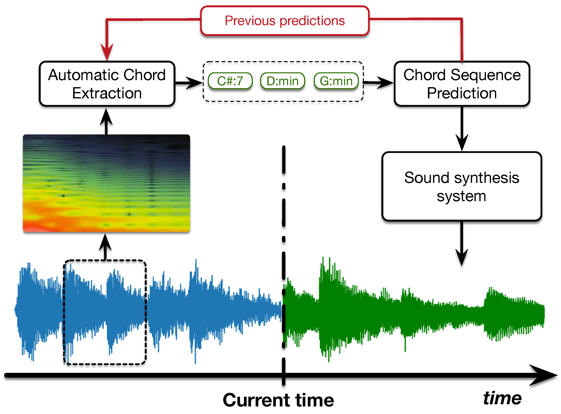
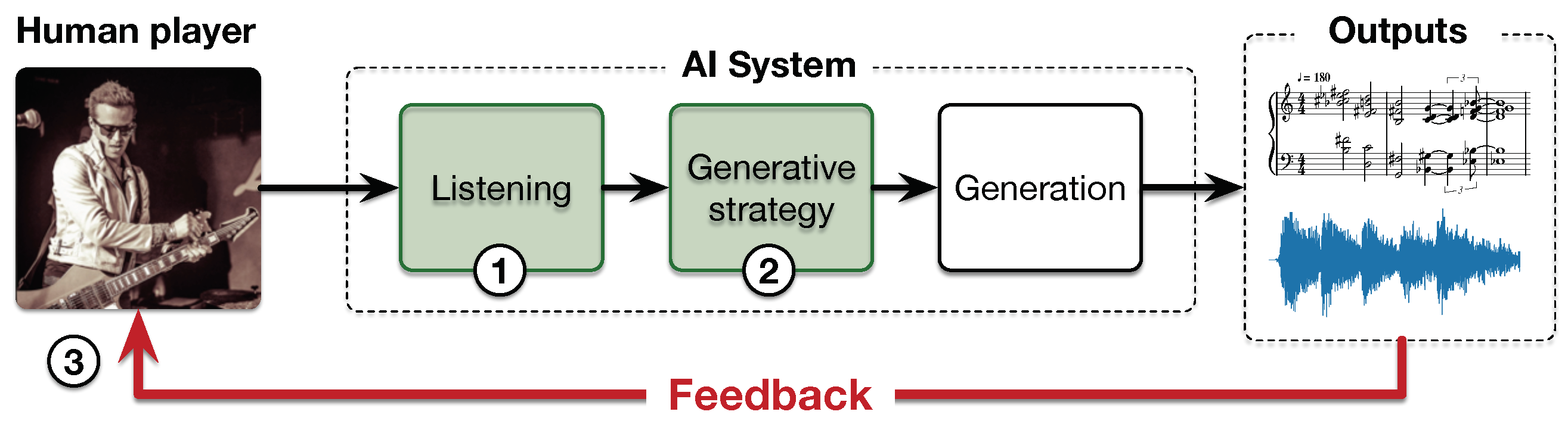
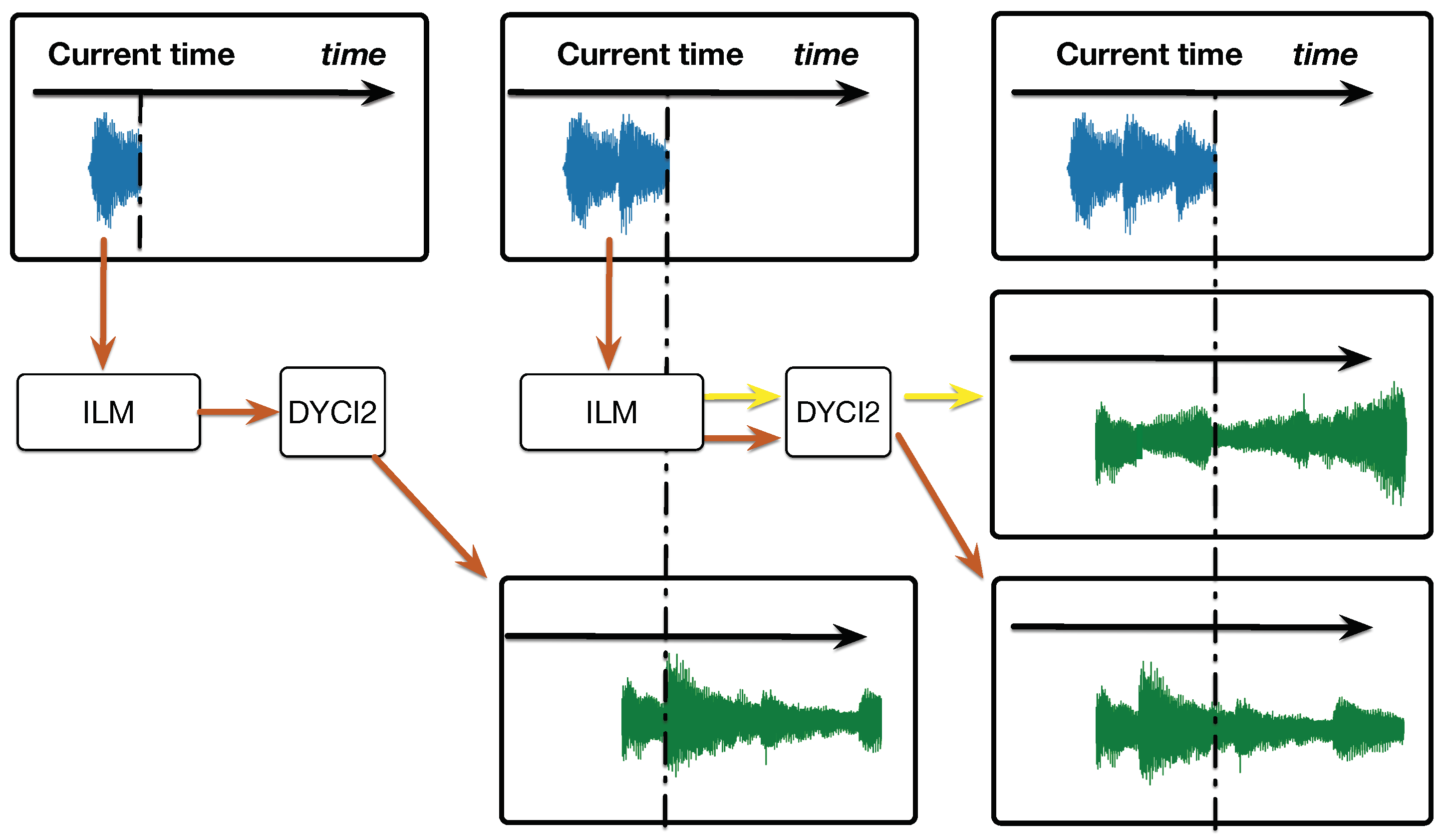
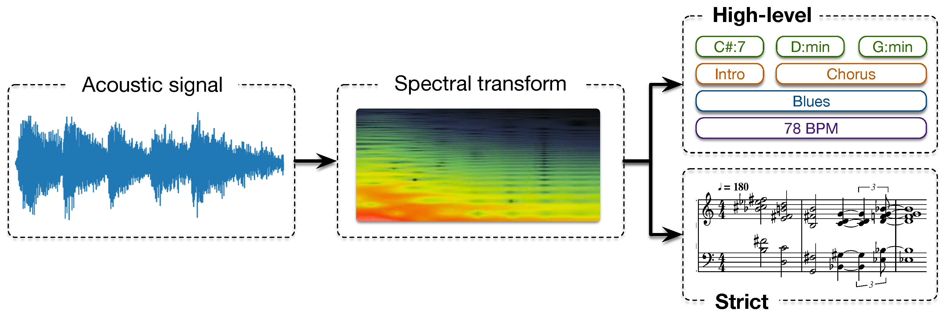
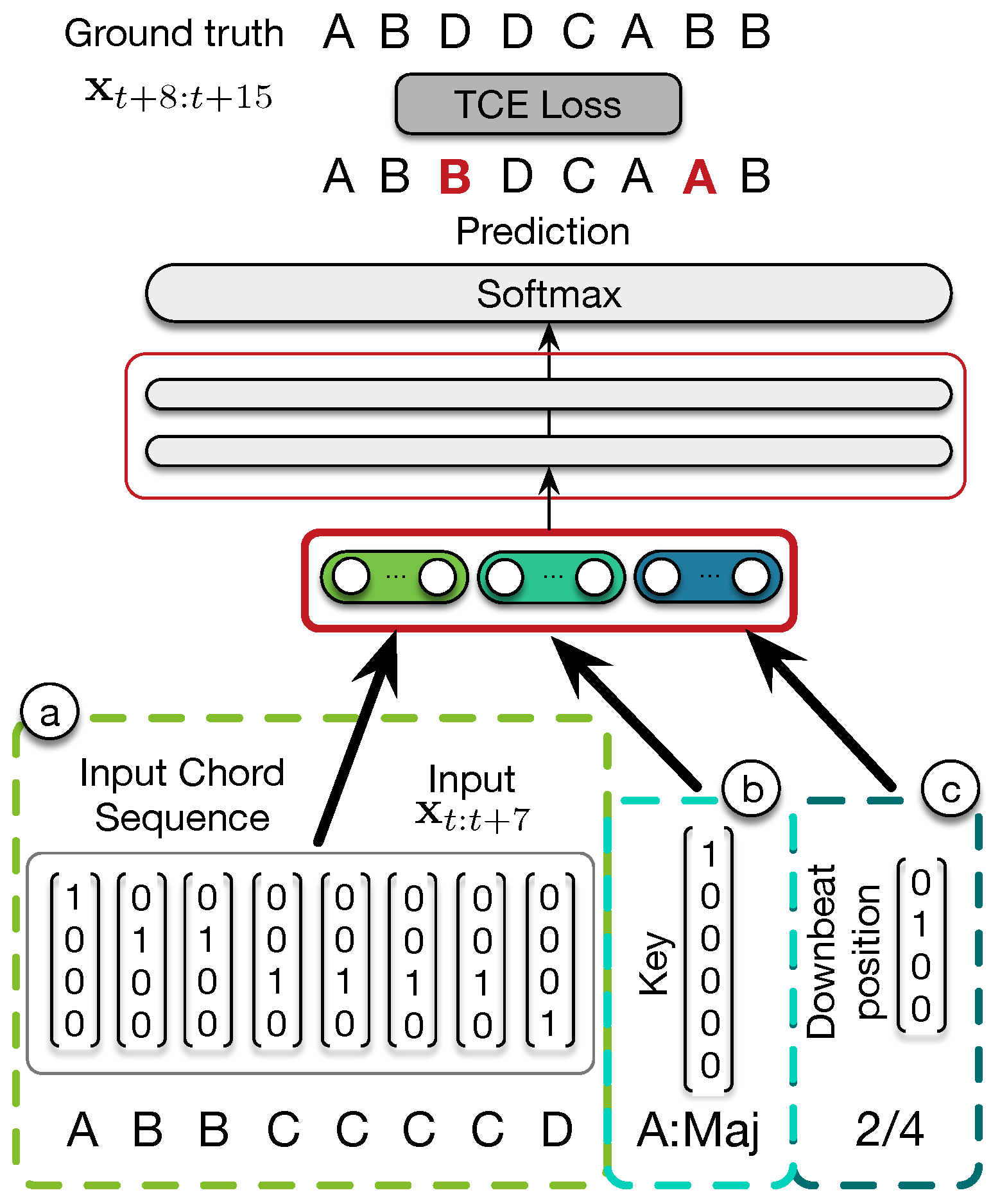
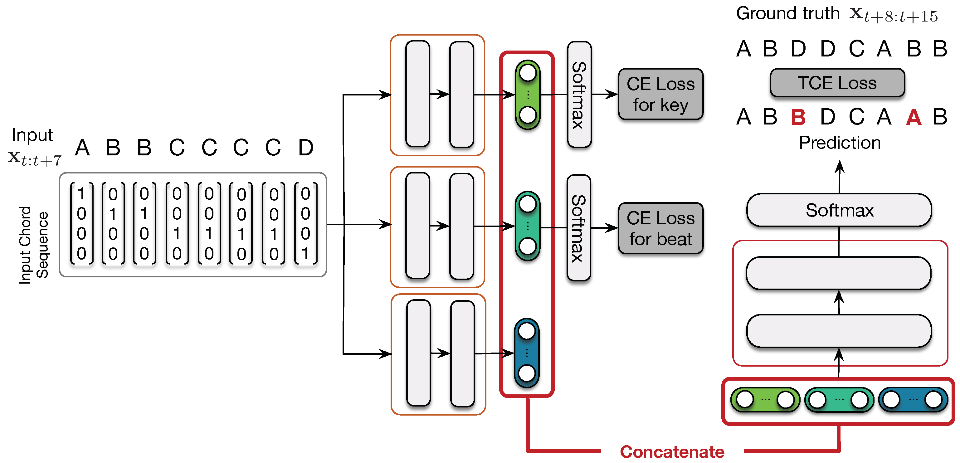
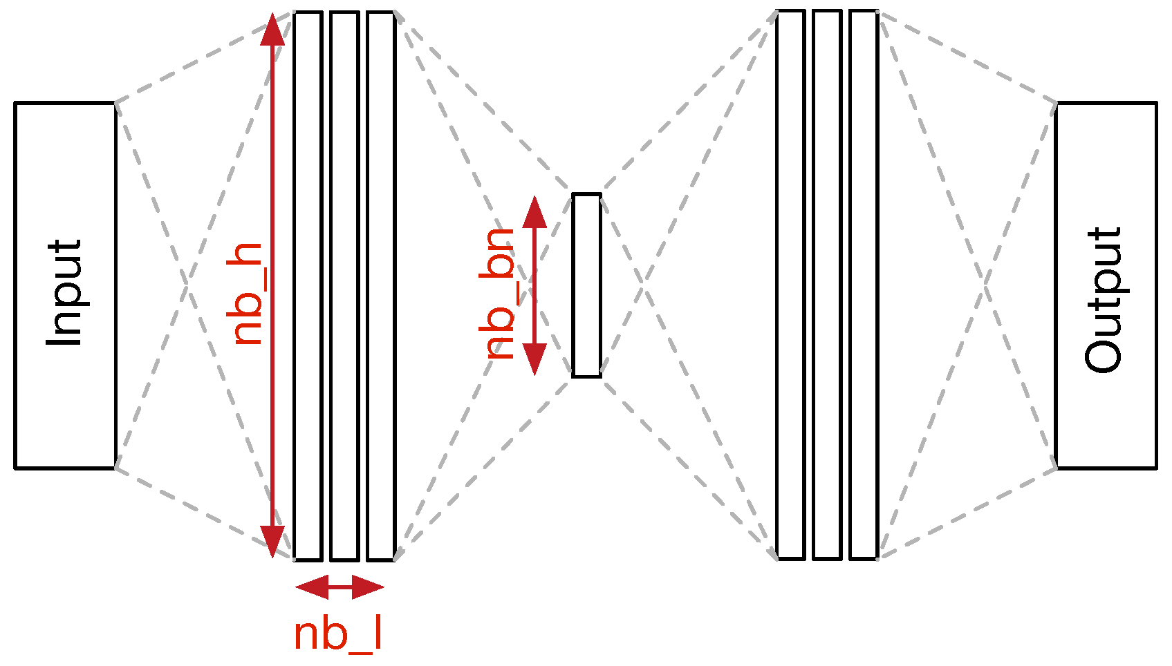