Wireless Power Transfer Using Double DD Coils

Abstract

This paper deals with a wireless power transfer system where a novel structure of transmitting/receiving double DD coils is applied. This system uses two identical double D (DD) transmitter coils stacked on each other to transfer power to two stacked receiver coils. The power is transmitted simultaneously and independently through both transmitter coils to the receiving coils. The magnetic field of the first coil does not interfere with the second coil. Both transmitter and receiver coils are placed on each other and occupy the same footprint, so there is no need for increased space. This can lead to an interesting wireless power transfer system—from single load to double the load and higher power transfer density.

1. Introduction

Research regarding wireless power transfer (WPT) has gained more interest due to the increase in the development of electric vehicles and portable mobile devices. Wireless power transfer can be used to charge and supply electric devices with different power ranges wirelessly, — from a couple of watts used to power up portable electronics such as medical equipment [1] and cell phones [2] to kilowatt ranges for use in charging electric vehicles [3,4,5,6]. Wireless power is transferred via an electromagnetic field. Methods for wireless power transmission differ from each other in the technology used to transfer power and in the distance the power should be transferred [7]. The distance of wireless power transfer is classified as near-field and far-field based on the wavelength (λ) of the electromagnetic radiation in comparison to the antenna dimensions (transmitter). Wireless charging of consumer electronics and electric vehicles is classified under near-field wireless power transfer [8]. The air gap between the transmitter and receiver is usually around a couple of centimeters to a couple of decimeters. The two main technologies used in near-field wireless transfer are Capacitive-wireless Power Transfer (CPT) and Inductive-wireless Power Transfer (IPT). While both technologies provide the opportunity to transfer a wide range of power (W to kW range), the IPT is more suitable for larger gaps and allows higher power density, while CPT is more suitable for smaller air gaps in the range of mm [7]. The main challenge of designing an IPT system is overall system efficiency. The transmitter and receiver coils are loosely coupled magnetically, so the coupling coefficient between coils is usually low. The system efficiency can be increased by increasing the operating frequency. In electrical vehicle applications, the operating frequency of the wireless power transfer is usually 85 kHz, which follows the resolution of the SAE International J2954 Taskforce about Wireless Power Transfer for Light-Duty Plug-in/Electric Vehicles and Alignment Methodology [9]. Maximum wireless charger power is limited by physical constraints of the lithium battery, such as the battery over-voltage and over-temperature. Battery modeling, observation, and the use of models in fast-charging algorithms are presented in [10,11]. The coupling coefficient is dependent on the distance and horizontal misalignment between the transmitter and receiver coils. The traditional coupler structure is unipolar and has poor horizontal misalignment tolerance [5,12]. Reference [13] proposed a new coupler structure called double D, or DD, which improves the horizontal misalignment tolerance. The DD coil is named after its shape compared to the classic spiral planar coil. It consists of two D-shaped coils, placed back-to-back. The DD coupler structure includes a polarized coil and mimics a polarized flux-pipe coil structure, without the double-sided magnetic field [14]. According to [13], horizontal misalignment tolerance along the y-axis is better than tolerance along the x-axis. To improve the design, another quadrature Q coil was added to the receiving DD coil. This resulted in a DDQ receiver coil with better horizontal misalignment tolerance along the x-axes. Reference [15] proposed a layered DD coupler structure (LDD), which improves the magnetic field and increases the power density. The DD coils in the LDD are positioned in a way so that the magnetic field adds up to a larger magnetic field constructively.

This paper presents a double DD coupler topology with a layered coil structure. Each transmitter and receiver includes two DD coils that are rotated by 90° around the z-axis. Due to the rotation between the two DD coils on the transmitter side, the coils are not coupled magnetically and can transfer power independently to their counterparts on the receiving side. This results in higher power density and uniform misalignment tolerance compared to a single DD coil. After the Introduction, Section 2 describes novel double DD coils that can be used in the same way as single-coil applications. Small-scale functional models are designed and evaluated to prove the feasibility of the double DD coils. Section 3 presents the IPT system structure. Section 4 describes the design process of a coupling coefficient measurement system and small-scale IPT system for experimental verification. Section 5 is divided into two parts: the first includes the measurements of inductance and the coupling coefficient of single and double DD coil structures in the x, y and z directions. The second includes the comparison of WPT systems based on single and double DD coil structures. Section 6 contains a discussion about the experimental results. Finally, Section 7 serves as a conclusion relating to the novelties described in this paper.

2. The Proposed Double DD Coil Design

This section describes novel double DD coils and their physical implementation on a small-scale test system. Both transmitter and receiver coils have the same design and the same parameters. The single DD coil structure and the proposed double DD coil structure are presented in Figure 1a,b, respectively. The coil structure in Figure 1a consists of a ferrite plate and a single DD coil with two terminals. The proposed double DD coil structure in Figure 1b consists of a ferrite plate, the first planar DD coil is noted as DD1, and the second planar DD coil is noted as DD2. Coils DD1 and DD2 are rotated 90° to each other. Each of the DD coils has two terminals; therefore, the proposed double DD coil has four terminals.

The DD coils in the single DD coil structure and DD coils in the proposed double DD coil structure have the same dimensions and the same parameters. The DD-shaped coils, shown in Figure 1a,b, have a polarized magnetic field; similar to but unlike the flux-pipe, the magnetic field is only radiated on the one side [15] (the side that is not shielded by the ferrite plate)—similar to ordinary non polarized planar spiral coils. This removes the need for other shielding and magnetic field cancelation, to follow safety standards, and to shield other components of the system.

When excited, the DD coil generates a polarized magnetic field. The main aspects of the magnetic fields of both single DD and double DD coil structures are presented in Figure 2a,b, respectively. Figure 2a presents the magnetic flux lines between the transmitter and receiver pad in the case of a single DD coil structure. The single DD transmitter coil generates the field marked with flux lines (yellow) and induces a voltage in the single receiver coil. Figure 2b presents the magnetic flux lines between the transmitter and receiver pad in the case of the double DD coil structure. DD1 generates the field marked with DD1 flux lines (yellow), and DD2 generates the field marked with DD2 flux lines (red). The main part of the DD1 field is perpendicular to the DD2 field. Due to the perpendicular nature of the DD coils’ fields, these are not linked magnetically. Similar cases are reported in [16,17], where magnetically uncoupled coils are used as a part of a resonator compensation structure. The DD1 field does not induce a voltage in the DD2 coil and vice versa. The DD1 coil would induce the voltage only in a coil that is not perpendicular to it. The coupling coefficient between the transmitter DD coil and receiver DD coil is maximized if both coils are aligned along the same axis.

Because transmitter coils DD1 and DD2 are magnetically uncoupled, they can be excited separate from each other, with different phases, different frequencies, and different currents. The transmitted magnetic fields do not interfere with each other. However, on the secondary, receiver side, the magnetic field does not interact if only the receiving pad is aligned correctly with the transmitting pad. Therefore, if the transmitter coils are excited separately, the receiver is dependent on rotation around the z-axis. Normally, in static WPT applications, in which the transmitter and receiver do not move, that should not be a problem, because the pads have the same orientation.

Practical implementation and measurements are needed to conform to the theory and working principles behind the proposed coil structure of double DD pads. A small-scale model was built to verify the principle of feasibility in a practical application. Figure 3a,b show the structure of the single and double DD coils. The size of the transmission pads was limited by the dimensions of the commercially available ferrite plates, which were square 100 by 100 mm. An ELECTROSOLA Litz wire with a nominal diameter of 0.071 mm and 50 strands was used to reduce the skin and proximity effects.

Implementation of the Layered Double DD Pads

A wound square transmission pad with a single DD coil structure is presented in Figure 3a. It consists of a single DD coil with two terminals and a ferrite plate. The wound square transmission pad with a double DD coil structure is presented in Figure 3b. It consists of two electrically separated DD coils with two terminals each.

The physical dimensions and properties of the small-scale testing coils are given in

Table 1. Transmission pad parameters.

Parameter	Value
Ferrite pad dimensions	100 mm × 100 mm
DD1 number of turns	18 (9 per D coil)
DD2 number of turns	18 (9 per D coil)
DD1 inductance (μH)	45
DD2 inductance (μH)	45
DD1 DC resistance (mΩ)	42
DD1 DC resistance (mΩ)	42

. The inductances of the DD coils were measured with an LRC meter at the frequency of 100 kHz. The coils were designed with an operating frequency of 85 kHz in mind. The DD1 and DD2 coils on the transmitting and receiving side had the same dimensions and same self-inductance. The difference in inductance between DD1 and DD2 came from the addition of the ferrite plate. The DD2 coil was positioned on the top of the DD1 coil. This resulted in lower self-inductance of the DD2 coil. If the DD1 and DD2 coils are nearly the same shape, and are positioned correctly perpendicularly, the coupling coefficient between them is zero. Practical tests show that the DD1 coil induced a negligible voltage level in the DD2 coil.

3. System Structure

The above-described double DD coil structure was evaluated in two stages. Both stages are presented in Figure 4. The first stage was a coupling coefficient measurement (evaluation) in the 3D space, illustrated with the block diagram in Figure 4a. The second stage was an evaluation of the IPT using the double DD coils, illustrated with the block diagram in Figure 4b. The IPT system was used to evaluate the inverter to rectifier power transfer and system efficiency. The double DD coil system was evaluated along with the single DD coil system. In both stages, the single and double DD coils were mounted on the mechanism of a repurposed 3D printer. This mechanism enabled the exact positioning of IPT transfer pads in a 3D space using proper hardware and software reconstructions. The primary transmitting side was mounted on the bottom platform, and the secondary receiving side was mounted on the top platform.

3.1. The Coupling Coefficient Measurement System

The coupling coefficient measurement system consisted of a high-frequency voltage source, a switch-manipulator for different mutual inductance evaluations, and a 3D positioning mechanism for positioning the transmitter and receiver pads. The measurement system is described further in more detail in Section 5.1.

3.2. The IPT System

An IPT system that uses double DD coils is similar to the basic IPT transfer system analyzed in [5,6] (Figure 4b). It is divided into two parts:

• A primary circuit on the transmitter side;
• A secondary circuit on the receiver side.

The primary side includes DC input voltage and a high-frequency inverter (transforms the DC input voltage to high-frequency AC voltage) that is used to drive the transmitter (TX) with a compensation circuit.

The secondary side includes the receiver (RX) coil and a compensation circuit. The RX coil receives the high-frequency AC voltage over the magnetic field. The AC voltage is afterward converted to DC voltage with the rectifier to supply DC voltage to the load. An important part of the circuit is a compensation circuit, which resonates with the inductor (transfer coil) and determines the resonant frequency of the IPT. The compensation circuit usually consists of a capacitor that is parallel (P) or in series (S) to the coil, so the capacitors C_Ti and C_Ri (i = 1,2) are added, as shown in Figure 5. Series–series compensation (SS) was used due to the necessity of a constant operating frequency [18].

4. The Experimental Set Benches

To test the IPT system concept, two experimental set-benches were fabricated and are shown in Figure 6a,b. The first one shown in Figure 6a stands for the setup for a coupling coefficient measurement between two transfer pads in a 3D space. The measurement set-bench included two coils and an inductance measurement circuit. The measurement circuit was based on an auto-balancing circuit [19]. The second one is shown in Figure 6b and stands for the setup for measuring the performance of the IPT system. In both cases, the transmitter and receiver coil were mounted on the previously mentioned 3D positioning mechanisms. The highlighted items in Figure 6a,b represent the measuring circuits, converters, and other parts of the systems. The primary and secondary sides of the IPT system relate to the TX and RX transmission pads. The transmission pads can have a single DD or double DD structure, as described in Section 2.

The parts of the IPT system that were mounted on the positioning mechanism are presented in Figure 6b. The inverter and auxiliary circuits of the synchronous rectifiers were powered by the controlled DC voltage source. The position of the 3D positioning mechanism and the output of the inverter were controlled by the PC application.

4.1. IPT System Parameters

A small-scale experimental IPT model was built to test the proposed double DD structure under the IPT application. The parameters of the IPT system are presented in

Table 2. System parameters.

Parameter	Value
Input voltage (max) UDC (V)	25
Input current (max) IDC (A)	2
Load RL (Ω)	20
TX compensation CT1 (nF)	75.8
TX compensation CT2 (nF)	85.9
RX compensation CR1 (nF)	76.9
RX compensation CR2 (nF)	85.6
Resonant frequency f0 (kHz)	85

. The system was designed with a resonant frequency of approximately 85 kHz. As stated before, the inductances of the DD1 and DD2 coils that compose the double DD coil structure differ from each other. Because of the differences in induction, series compensation capacitors C_Ti and C_Ri must have different values for the system to resonate at the same resonant frequency. Two resonators are formed via the magnetically linked transmitter L_Ti and L_Ri coils with their respective compensation circuits C_Ti and C_Ri (i = 1,2). To protect the system from exceeding the current limit, the DC power source was current limited to 2 A. To reduce the hard switching losses of the inverter, the Zero Voltage Switching (ZVS) technique could be applied [20,21]. In the ZVS region, the IPT system must work with a frequency above the resonant frequency the resonator circuit was designed for. The resonator shows inductive load properties and the current lags the voltage. This is the condition that enables ZVS.

4.2. IPT System Description

Typically, an IPT system consists of one transmitting and one receiving coil. Usually, a half-bridge or a full-bridge transistor inverter is used to drive the TX coil [22]. The full-bridge inverter has the added capability to control the TX coil voltage using Phase Shift Pulse Width Modulation (PSPWM), and so, the voltage at the output of the inverter [6].

Double DD coils can be considered as two separated transmission coils, which transform our system from a system with a single transmitter–receiver to a multi transmitter–receiver system. In a system with multiple coils, each transmitter coil can be driven by a separate full-bridge inverter. The full-bridge inverter consists of two half-bridge transistor legs. Each leg can drive one resonator circuit. The proposed circuit is presented on the left side in Figure 5.

4.2.1. High-Frequency Inverter

Each coil is driven by a separated half-bridge inverter, powered up from the same DC voltage source. Each of the two DD coils can be excited by the same frequency, or even by two different frequencies. The working frequency of the system is determined by the inductance of the coils and the capacitance of the compensation circuit. The high-frequency inverter was designed for maximum transfer power around 50 W. The circuit of the high-frequency inverter consists of four Metal–Oxide–Semiconductor Feld-Effect-Transistors (MOSFET) (FDS5672, ON Semiconductor) and two isolated bridge drivers (SI8275BBD-IS1, Skyworks). It also includes input and output current measurement shunt resistors (R_sh = 20 mΩ) and voltage measurement circuits for use in measuring voltages up to 50 V.

4.2.2. Driving the Inverter MOSFETs

The MOSFETs in a high-frequency inverter are controlled with a control board (LAUNCHXL-F28379D, Texas Instruments) with a Digital Signal Processor (DSP TMS320F28379D). The control card generates 87 kHz phase-shifted PWM signals for transistor drivers. The frequency of the PWM signal can be changed using a PC application. The DSP unit also has analog-to-digital converters (12-bit ADC). The digitalized measurement data are sent through the virtual COM port to the PC for further visualization. The DSP presents the interface between the computer and the IPT system.

4.2.3. Primary and Secondary Compensation Circuits

The primary and secondary resonators are designed to resonate with IPT transfer coils at frequencies around 85 kHz. The primary resonator circuit includes two series resonant capacitors, one for each of the two TX DD coils. On the secondary side, there are two resonators with a single resonant capacitor. Each one of the secondary resonators is connected to a synchronous rectifier.

4.2.4. Synchronous Rectifier

The receiving side of the IPT system with double DD coils can be implemented with two secondary resonator circuits and two rectifiers. On the contrary, the single DD coil can only implement one secondary resonator circuit and a MOSFET-based synchronous rectifier. A system with double DD coils can also power up two separate loads. The proposed receiving side circuit is presented on the right side in Figure 5. Each circuit consists of a receiver DD coil, a compensation capacitor, a synchronous transistor rectifier, and load [22]. The synchronous rectifiers were designed for rectification up to 50 W. The conventional rectier diodes are replaced with four MOSFETs (FDS5672, ON Semiconductor). The synchronous rectifier achieves higher efficiency compared to a conventional diode rectifier by replacing the forward voltage drop on diode and diode resistance for a transistor with smaller R_ON resistance. The transistors are driven with four synchronous rectifier drivers (TEA1993TS, NXP Semiconductors), one for each transistor. Each rectifier also has current and voltage measurement circuits.

5. Simulation and Experimental Results

The simulation and experimental results are presented and a comparison between single- and double-layered IPT systems is shown. Using equivalent circuits, the coupling coefficient was analyzed and measured in the 3D space. The magnetic flux density of single and double DD coils was simulated and compared using the EM Field solver. Finally, the efficiency evaluation and power transfer measurements of the single DD coil and double DD coil system are presented. Measurements on the system were performed at different distances between the transfer and receiver coils, different system frequencies, and different loads. The TX and RX pads were positioned using a 3D measurement rig.

5.1. Coupling Coefficient Measurement between Double DD Pads

To evaluate the coupling coefficient between the transmitting and receiving pads, both pads were mounted on a computerized 3D measurement rig that enabled automated measurements of mutual inductance in a 3D space. Because the proposed double DD pad consists of two separated DD coils, every point in the space requires two mutual induction measurements. A well-known method (from the textbook) [23] was used to evaluate the mutual inductances between the transfer pads. 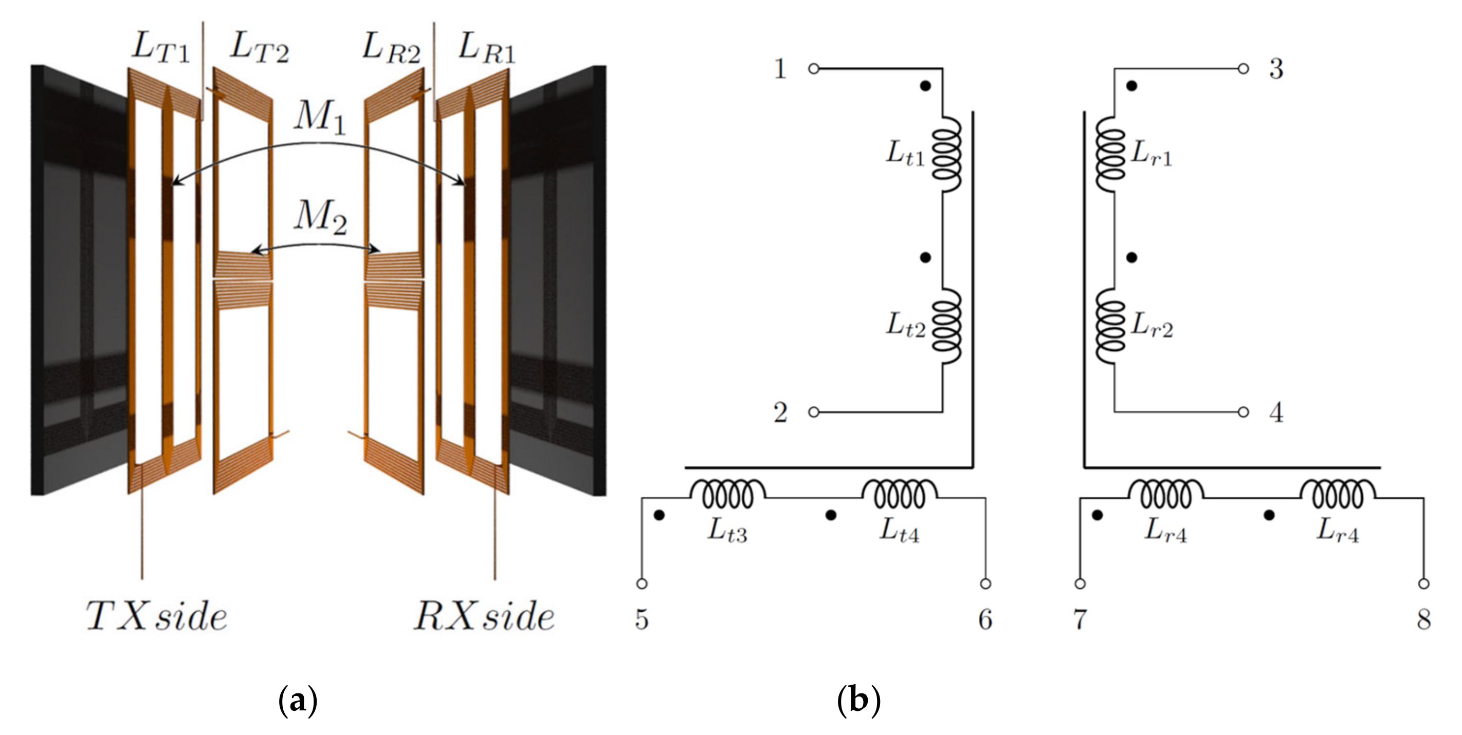The measurement schemes can be simplified, as is shown in Figure 7a−d.

The DD coils on the transmitter and the receiver side were connected in series and two measurements of circuit inductance were performed. Transmitter and receiver coils could be connected in series in constructive or destructive mutual inductance. In the case of constructive mutual inductance, the measured value is denoted as L′, and in the case of destructive mutual inductance, the measured value is denoted as L″.

Mutual inductance between the transferred pad is presented in Figure 7a and the electrical scheme of the coils is presented in Figure 7b. The transmitter DD coil can be divided into two coils with inductance $L_{t1} (L_{t3}) \mathrm{and} L_{t2} (L_{t4})$ (Figure 7c). Similarly, the receiver DD coil can be divided into two coils with inductance $L_{r1} (L_{r3}) \mathrm{and} L_{r2} (L_{r4})$. The flowing mutual inductance measurement is presented for the two D coils of the DD1 transmitter coil. In the case of constructive mutual inductance, mutual inductance between these two parts and their self-inductance adds up to the inductance L′, which can be measured. Likewise, in the case of destructive mutual inductance, L″ can be measured. Using these two measurements, L′ and L″, the mutual inductance between two parts of a single transmitter DD coil $L_{t1} (L_{t3}) \mathrm{and} L_{t2} (L_{t4})$ can be evaluated as follows:

$$L´=L_{t1}+L_{t2}+2M_{t12},$$

(1)

$$L˝=L_{t1}+L_{t2}-2M_{t12},$$

(2)

and after using (1) and (2), the local transmitter DD coil mutual inductances can be obtained:

$$M_{t12}=M_{r12}=\frac{L\prime -L″}{4}$$

(3)

This information from (1) to (3) can be used for TX and RX coil design. The earlier step concludes that the measured inductances between the terminals of the DD coil are slightly different from the sum of the inductance of both spiral coils that make the DD coil. For the further analyses, the measured L’ is denoted with L′ = L_Ti = L_Ri (i = 1,2), as shown in Figure 7b. The coupling coefficient between the TX and RX pads can be evaluated as shown in Figure 7c. The mutual inductances, M_i, can be obtained via the measurement of L_X1 and L_X2 and then calculated as follows:

$$\begin{array}{l}{L}_{X1}=L_{Ti}+L_{Ri}+2M_i,\\ L_{X2}=L_{Ti}+L_{Ri}-2M_i,\end{array}$$

(4)

where L_Ti (L_Ri) (i = 1,2) shows the resulting inductances of both the primary and secondary sides of the newly established transformer (Figure 7d), L_X1 is measured inductance in the case of constructive mutual inductance between the TX and RX coil, and L_X2 is the measured inductance in the case of destructive mutual inductance between the TX and RX coil. In the above analysis, it is supposed that the coils L_t1, L_t2, L_t3, L_t4, L_r1, L_r2, L_r3, and L_r4 are designed with the same number of turns, so, after measuring the inductances L_X1 and L_X2, both mutual inductances M₁ and M₂ (because M₁ = M₂), can be evaluated as:

$$M_1=M_2=\frac{L_{X1}-L_{X2}}{4}$$

(5)

and the coupling coefficient k₁ and/or k₂ could be calculated in every x, y and z point as follows:

$$k_1(x,y,z)=k_2(x,y,z)=\frac{M_i(x,y,z)}{\sqrt{L_{Ti}(x,y,z)L_{Ri}(x,y,z)}}$$

(6)

So, three inductances, L’, L_X1, and L_X2, should be measured to evaluate the coupling coefficient for single and double DD TX–RX coil structures. The DD coils on the transmitter side are placed perpendicularly, $L_{T1}\perp L_{T2}$, and the same on the receiver side, $L_{R1}\perp L_{R2}$, so, due to this, the coupling coefficient between them is near to zero, $k_{L_{T1}\perp L_{T2}}\approx k_{L_{R1}\perp L_{R2}}\approx 0$, and is neglected in further analyses.

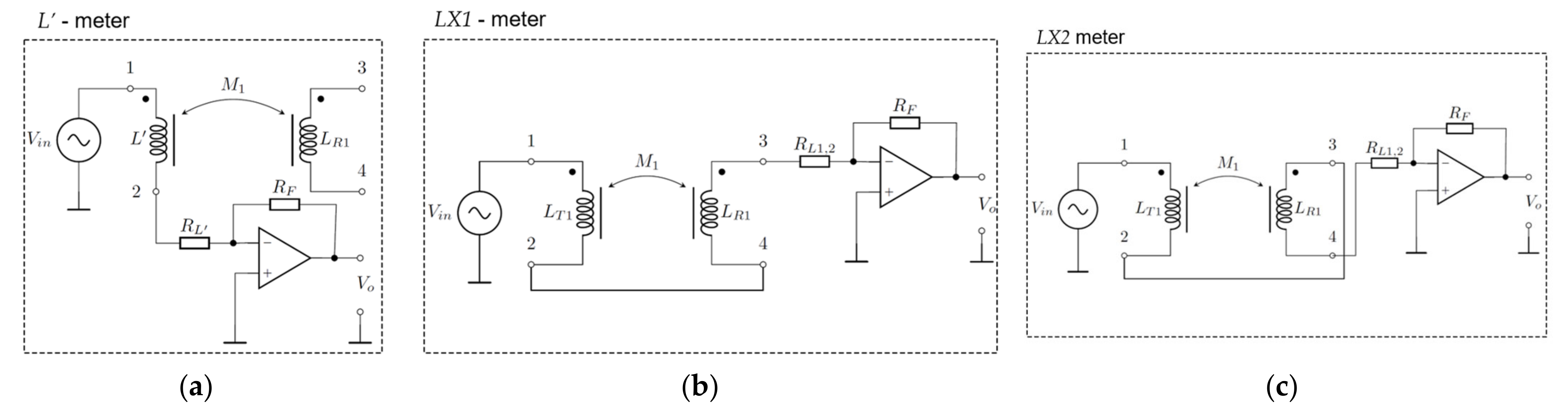
5.2. Measurement of L′, L_X1 and L_X2′ Inductances

The inductance measurement method is based on an auto-balancing circuit, which converts current through unknown impedance of inductance L into voltage using an operational amplifier, as presented in Figure 8 [20].

Figure 8a presents a measurement circuit for measuring self-inductance L′ between terminals 1 and 2 in the case of the DD1 TX coil (between terminals 5 and 6 in the case of the DD2 TX coil). Figure 8b presents a measuring circuit for the measurement of L_X1, and Figure 8c presents a measurement circuit for measuring L_X2. At each x, y and z point, the coupling coefficient k is evaluated for all three inductances.

The relation between the input and the output voltage can be described as follows:

$$\left|\frac{V_O}{V_{in}}\right|=\frac{R_F}{\sqrt{R_L{}^2+{\omega }^2{L}^2}}$$

(7)

where R_F is the value of the resistor used for voltage amplification, L is the inductance of the measured inductor, and R_L is the resistance of the measured coil circuit. Under the assumption that the resistance of the measured coil circuit is near zero ($R_L\approx 0$), Equation (7) can be simplified to:

$$\left|\frac{V_O}{V_{in}}\right|=\frac{R_F}{\omega L}$$

(8)

where V_in stands for the high-frequency voltage source of the sinusoidal excitation signal at the input of the circuit $V_{in}\left(\omega t\right)=\widehat{V}\sin \left(\omega t\right)$, ω = 2πf, and f = 100 kHz. Manipulating (8) the inductance L can be obtained as:

$$L=\frac{R_F}{2\pi f\left|\frac{V_o}{V_{in}}\right|}$$

(9)

The circuit was designed for measurements of inductance between 2.59 μH to 2.38 mH at 100 kHz frequency. The induction of the coil circuit measured with this method was up to 150 μH, which is within the range of the measurement circuit.

5.3. Measurement of the Coupling Coefficient on the x-y Plane

Coupling coefficient measurements were performed using a 3D spatial positioning system. In each position, the inductances of L′, L_X1 and L_X2 were measured and transferred to the PC via serial communication. The calculated coupling coefficient was written and exported to a Comma Separated Value (CSV) file, and afterward visualized in graph form. The coupling coefficient of the single and double DD pad structure was measured on the x-y plane at three different z positions. A single DD coil has the same orientation as the DD1 coil of the double DD coil structure. Therefore, the results for the single DD coil and the results for the DD1 coil in the double DD coil structure were equal. The results are presented in Figure 9 and Figure 10. Measurement was performed on the x-y plane by misaligning the coils in a 50 mm square around the perfectly aligned position. 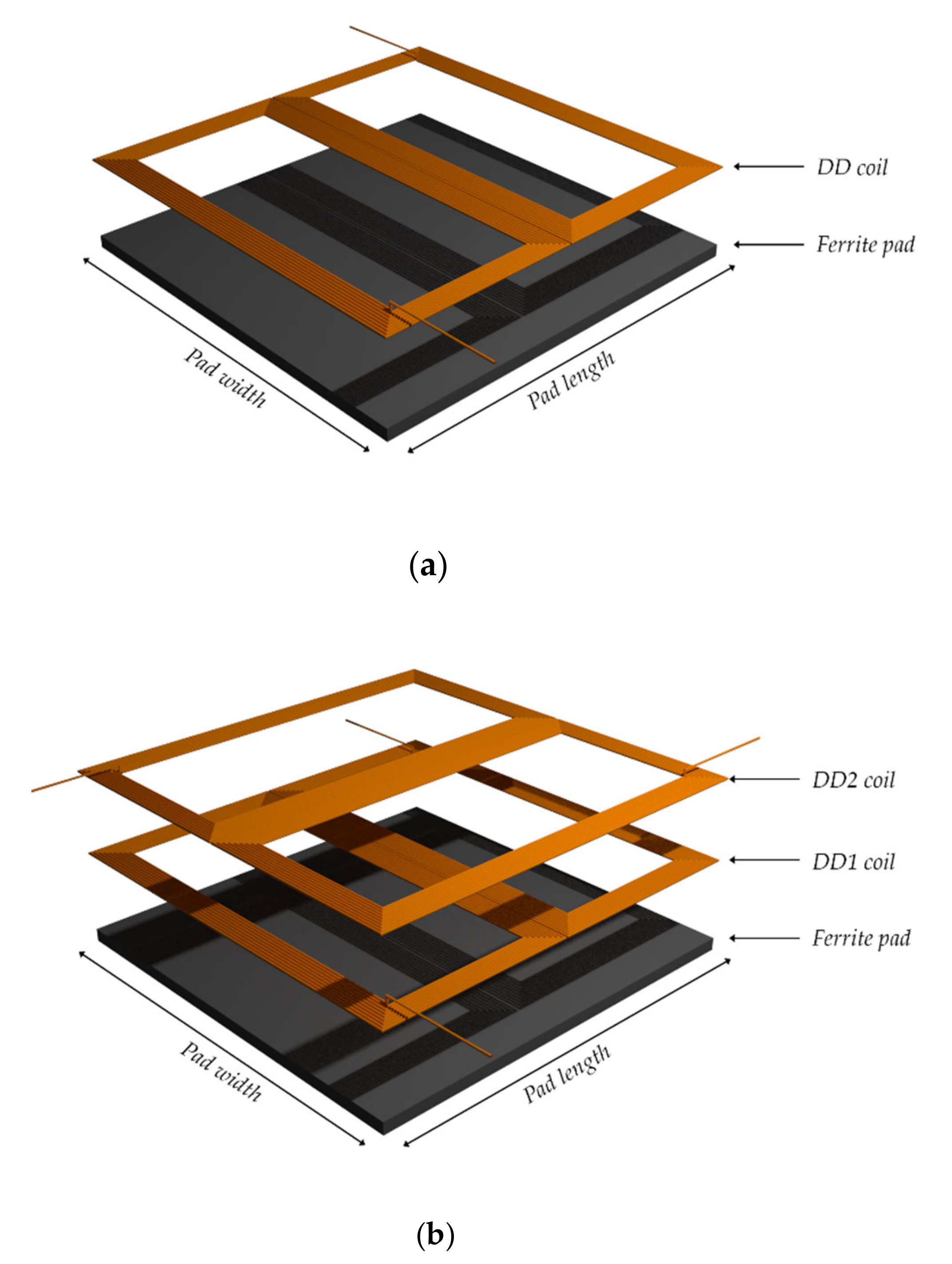The single DD and double DD coil measurement results, considering the coupling coefficients k, k₁, and k₂ at three different z distances between the pads, are presented in Figure 9 and Figure 10, respectively. The coupling coefficient of the DD coil in the single DD coil structure and DD1 coil in the double DD coil structure is marked with a blue surface, and the coupling coefficient of the DD2 coil of the double DD coil structure is marked with an orange surface.

The coupling coefficient is the greatest when both coils are aligned perfectly in an ideal case. Due to the flux-pipe-like magnetic field, the coefficient decreases more in one horizontal direction than in the other horizontal direction. The direction in which the coupling coefficient is less impacted by misalignment is the direction parallel to the main magnetic flux of the coil. In the case of the single DD coil, this direction is along the x-axis. In the case of the double DD coils, the coupling coefficient of the DD1 coil has a greater tolerance for change in the x-direction and the coupling coefficient of the DD2 coil has a greater tolerance for change the y-direction.

To differentiate between the measurements of the DD (DD1) and DD2 coils, the measurements of L′, L_X1 and L_X2 are marked with additional indexes. Self-inductance L′ of the transmitter coil is marked as L_T1 for the DD1 coil and L_T2 for the DD2 coil. Self-inductance of the receiver coil is marked as L_R1 for DD1 coil and L_R2 for DD2 coil. In the case of the evaluation of mutual inductance between the two DD (DD1) coils, the value of L_X1 is denoted by L_X11. Similarly, the value of L_X2 is denoted by L_X21. When the mutual inductance between the two DD2 coils is evaluated, the value of L_X1 is denoted by L_X12 and the value of L_X2 is denoted by L_X22. The measurement data for the DD (DD1) and DD2 coils when misaligned along the x-axis at y = 0 and z = 25.3 mm are presented in

Table 3. Coupling coefficient measurements of the DD (DD1) and DD2 coils in the x-axis at y = 0 and z = 25.3 mm.

Parameter					Value
x (mm)	−25	−22	…	−2	0	2	…	22	25
DD and DD1
LT1 (μH)	47.86	47.95	…	48.13	48.12	48.12	…	47.93	47.87
LR1 (μH)	47.88	47.96	…	48.13	48.13	48.12	…	47.94	47.89
LX11 (μH)	116	117.3	…	121.3	121.4	121.4	…	117.9	117.1
LX21 (μH)	75.48	74.52	…	71.22	71.10	71.08	…	73.84	74.42
M1 (μH)	10.13	10.70	…	12.52	12.58	12.58	…	11.02	10.67
k1	0.21	0.22	…	0.26	0.26	0.26	…	0.23	0.22
DD2
LT2 (μH)	44.06	44.27	…	44.75	44.76	44.76	…	44.35	44.22
LR2 (μH)	43.59	43.8	…	44.26	44.26	44.26	…	43.79	43.66
LX12 (μH)	94.03	98.45	…	114.1	114.3	114.3	…	100.2	97.27
LX22 (μH)	81.27	77.69	…	63.92	63.74	63.74	…	76.08	78.49
M2 (μH)	3.19	5.19	…	12.55	12.64	12.64	…	6.03	4.70
k2	0.07	0.12	…	0.28	0.28	0.28	…	0.14	0.11

. The measurement data for the DD (DD1) and DD2 coils when misaligned along the y-axis at x = 0 and z = 25.3 mm are presented in

Table 4. Coupling coefficient measurements of the (DD) DD1 and DD2 coils in the y-axis at x = 0 and z = 25.3 mm.

Parameter					Value
y (mm)	−25	−22	…	−2	0	2	…	22	25
DD and DD1
LT1 (μH)	47.39	47.58	…	48.12	48.13	48.14	…	47.75	47.63
LR1 (μH)	47.44	47.64	…	48.11	48.12	48.11	…	47.69	47.57
LX11 (μH)	101.6	105.9	…	121.2	121.4	121.4	…	106.8	104
LX21 (μH)	88.06	84.54	…	71.26	71.1	71.1	…	84.08	86.4
M1 (μH)	3.39	5.34	…	12.49	12.58	12.58	…	5.68	4.40
k1	0.07	0.11	…	0.26	0.26	0.26	…	0.12	0.09
DD2
LT2 (μH)	44.62	44.7	…	44.95	44.96	44.96	…	44.86	44.81
LR2 (μH)	44.07	44.16	…	44.38	44.38	44.38	…	44.24	44.2
LX12 (μH)	108.5	109.7	…	114	114.1	114.1	…	110.8	110.1
LX22 (μH)	68.88	68.02	…	64.66	64.58	64.58	…	67.4	67.92
M2 (μH)	9.91	10.42	…	12.34	12.38	12.38	…	10.85	10.55
k2	0.22	0.23	…	0.28	0.28	0.28	…	0.24	0.24

. In Table 3 and Table 4, the values of L_T1, L_T2, L_R1, L_R2, L_X11, L_X12, L_X21 and L_X22 were measured using the auto-balancing circuit. Coupling coefficient k₁ was calculated from M₁ and self-inductance L_T1 and L_R1, and coupling coefficient k₂ was calculated from M₂ and self-inductances L_T2 and L_R2. Compared to a single DD coil (k₁ or just k), the double DD coil has two coupling coefficients (k₁ and k₂) independent of each other. This allows for the possibility of transmitting power independently through each of the DD coils in the double DD coil structure. Theoretically, this allows the double DD coil structure to send twice as much power on the same surface as the single DD coil. 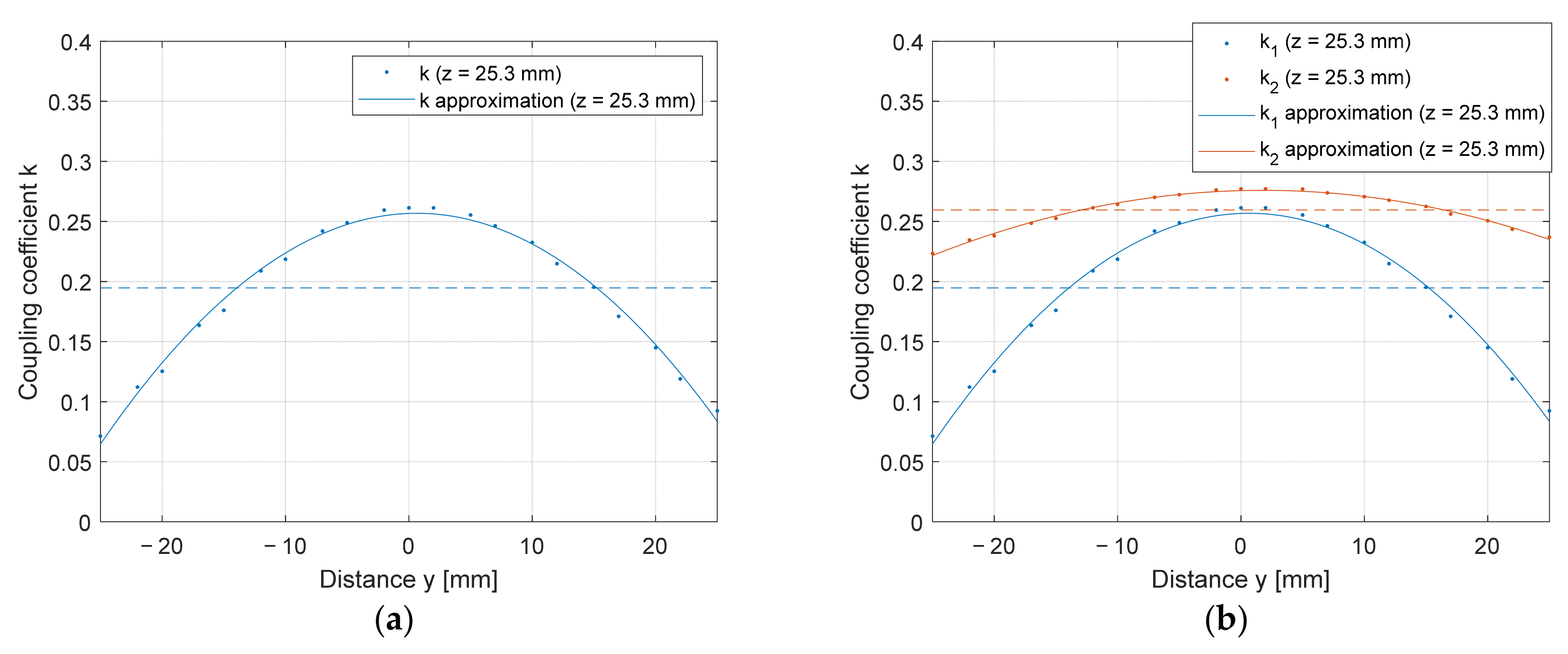Figure 11 and Figure 12 present a slice of a 3D graph with data from Table 3 and Table 4 for single and double DD coils at z = 25.3 mm. The DD coil of the single DD coil structure is the same as the DD1 coil in the double DD coil structure. Figure 11a presents the coupling coefficient of a single coil when the coil is perfectly aligned along the y-axis (y = 0 mm), and Figure 10b presents the coupling coefficient of a double DD coil when the coil is perfectly aligned along the y axis (y = 0 mm). Figure 11a presents the coupling coefficient variation of the single DD coil when the coil is perfectly aligned along the x-axis (x = 0 mm). Figure 11b presents the coupling coefficient variation of the double DD coil when the coil is perfectly aligned along the x-axis (x = 0 mm).

It is difficult to obtain relevant results from the 3D diagrams in Figure 9 and Figure 10, so it is better to extract the relevant information from the 2D diagrams, as shown in Figure 11 and Figure 12. On the diagrams, the data calculated from the measurement points are marked with dots. Quadratic function approximations of the coupling coefficient are marked with a full line. The dashed lines stand for the average coupling coefficient of the DD coils in the single DD and double DD coil structures. In Figure 11b, the DD1 coil in the double DD coil structure has the same misalignment tolerance as the coil in the single DD coil structure. The DD2 coil of the double DD coil structure had a worse horizontal tolerance along the x-axis compared to the DD1 coil. This also reflects in the lower average coupling coefficient k₂ of the DD2 (orange dashed line) when compared to the average coupling coefficient k₁ of the DD1 coil (blue dashed line). On the other hand, in Figure 12b, the DD2 coil of the double DD coil structure performed better than the DD coil in the single DD coil structure along the y-axis. Similarly, it also performed better than the DD1 coil of the double DD coil structure. This reflects in the lower average coupling coefficient k₁ of the DD1 (blue dashed line) when compared to the average coupling coefficient k₂ of the DD2 coil (red dashed line). The DD1 coil of the double DD coil structure performed the same as the DD coil in the single DD coil structure. From Figure 11a and Figure 12a, it can be concluded that the horizontal misalignment along the x-axis had less impact on the coupling coefficient of the single DD coil. On the other hand, the coupling coefficient of the single DD coil was reduced drastically when the coil was misaligned along the y-axis. The two DD coils in the double DD coil structure also showed the same properties as the single DD coil, although along two different axis directions.

In the case of misalignment along the x-axis, the DD1 coil performed better than the DD2 coil (Figure 12b). In the case of misalignment along the y-axis, the DD2 coil performed better than the DD1 coil (Figure 12b). Because efficiency is dependent on the coupling coefficient, the IPT system with the single DD coil performed better when it was misaligned along the x-axis compared to the system with the double DD coil. In the case of misalignment along the y-axis, the IPT system with the double DD coil kept higher efficiency compared to the single DD coil system. The coupling coefficients from Figure 11 and Figure 12 can be approximated using quadratic functions (two sets of equations for each of the two DD coils):

$$k_1\left(x,y=0\hspace{0.17em}\mathrm{mm},z=25.3\hspace{0.17em}\mathrm{mm}\right)=-7.084\cdot {10}^{-5}{x}^2+2.159\cdot {10}^{-4}x+0.2602$$

(10)

$$k_1\left(x=0\hspace{0.17em}mm,y,z=25.3\hspace{0.17em}mm\right)=-2.92\cdot {10}^{-4}{y}^2+3.759\cdot {10}^{-4}y+0.2567$$

(11)

$$k_2\left(x,y=0\hspace{0.17em}mm,z=25.3\hspace{0.17em}mm\right)=-3.164\mathrm{E}\cdot {10}^{-4}{x}^2+4.7019\cdot {10}^{-4}x+0.2787$$

(12)

$$k_2\left(x=0\hspace{0.17em}mm,y,z=25.3\hspace{0.17em}mm\right)=-7.586\cdot {10}^{-5}{y}^2+2.67\cdot {10}^{-4}y+0.2757$$

(13)

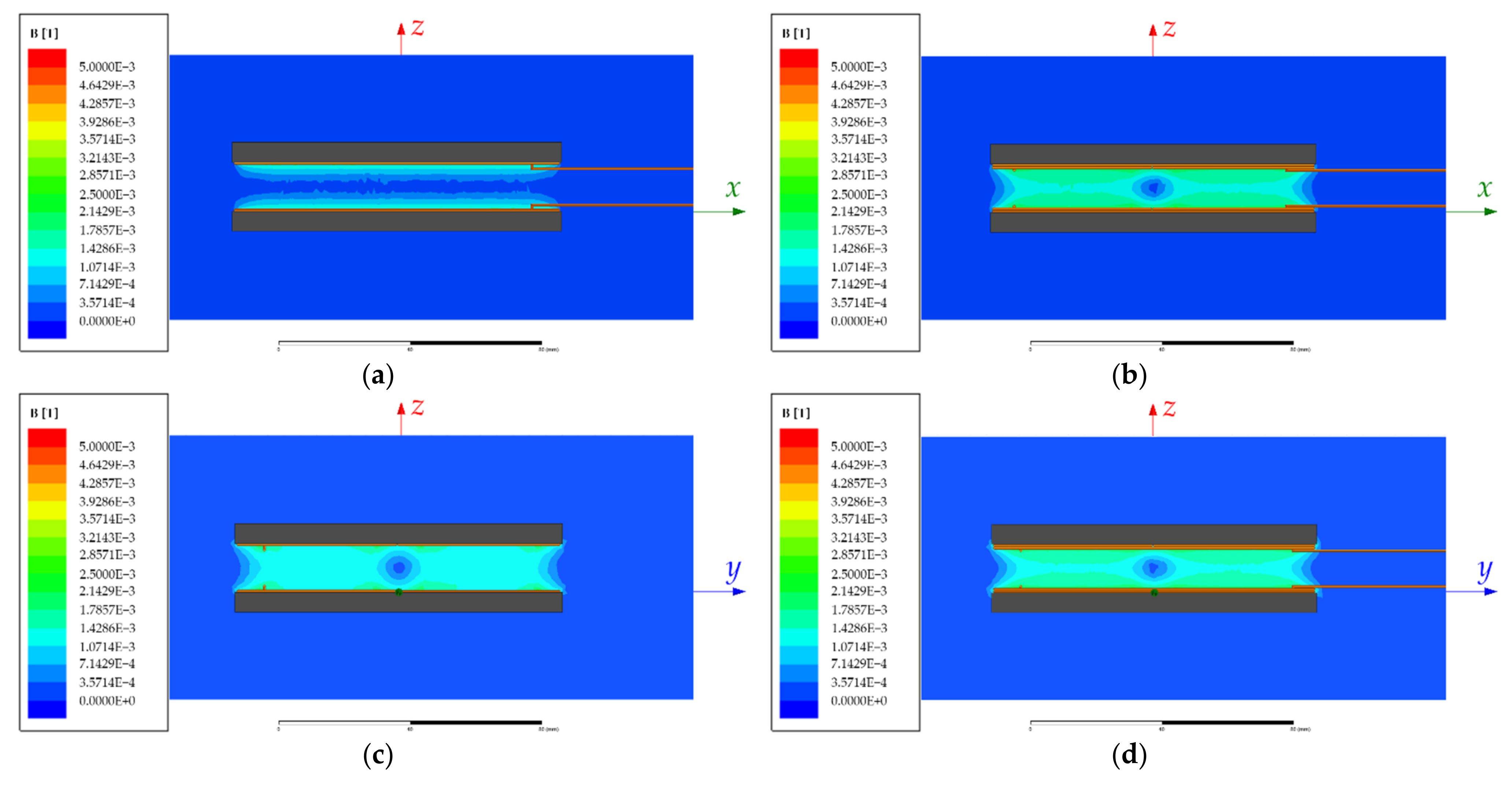
5.4. Simulation of Magnetic Flux Density

The FEM simulation software Ansys Maxwell was used to test the proposed IPT pad design. The transmitter and receiver pads were modeled in a 3D space and had the same dimensions and design as the manufactured coils of the experimental system. The distance between the pads was set to 15.3 mm (in the z-axis, x = 0 and y = 0), and the excitation current for each of the DD coils was set to 1 A. The simulation was used to compare the magnetic flux density of the single and double DD coils.

Figure 13a,c,e present the calculated magnetic flux density of the single DD coil in three vertical planes. Figure 13b,d,f present the magnetic flux density of the layered double DD coils, also in three vertical planes. The magnetic flux density for the single DD coil in the x-z, y-z, and y-x plane are shown in Figure 13a,c,e, respectively. Figure 13b,d,f show the magnetic flux density in the x-z, y-z, and x-y planes for the double DD coils, respectively. From the simulation results, it can be concluded that the magnetic flux density of the double DD coil in the x-z plane is like the magnetic flux density of the double DD coil in the y-z plane. The double DD coil therefore also generates symmetrical magnetic flux density in both the x-z and y-z planes. So, the flux densities are symmetrical when horizontal misalignment is applied across the x and y axes.

In the case of the single DD coil, the magnetic flux density was not symmetrical. Therefore, a parallel can be seen between the magnetic flux density simulation results and the coupling coefficient measurement in the 3D space. Due to the asymmetrical magnetic field of the single DD coil, the coupling coefficient was also not symmetrical. On the other hand, the magnetic flux density of the double DD coil showed symmetry along the x-z and y-z planes, which was also the case with the average coupling coefficient value. The biggest difference in magnetic flux density between the single DD and double DD coil is on the x-y plane, as shown in Figure 13e,f. The magnetic flux density generated by the single DD coil is weaker than the one generated by the double DD coil. The magnetic flux density of the double DD coil also cancels itself out in the top left and bottom right coil quadrant. The receiver coils of the double DD coil structure receive two different components of the generated magnetic field. The DD1 coil receives the y component and the DD2 coil receives the x component. In the case of the single DD coil, the receiver coil only captures the y component of the magnetic field.

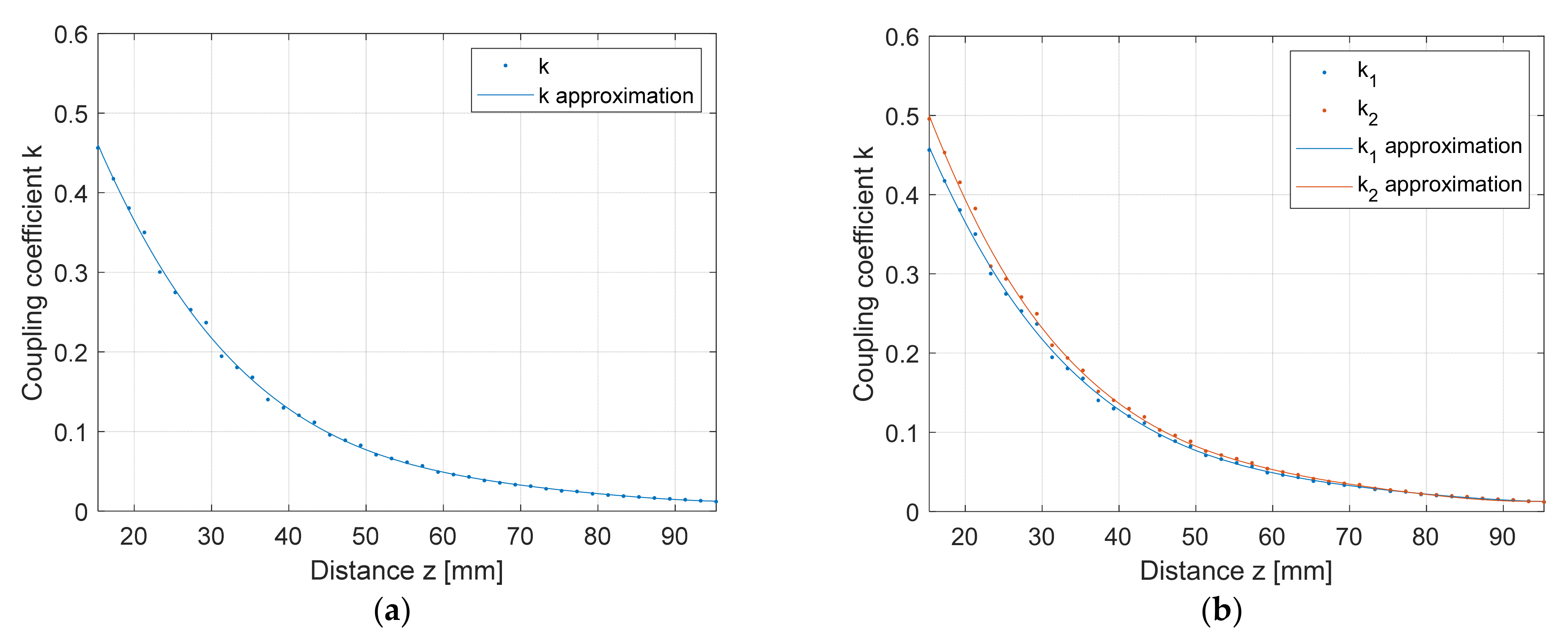
5.5. Measurement of the Coupling Coefficient in the z Direction

The vertical z-axis measurement was performed at distances between 15.3 mm and 95.3 mm with 2 mm steps. Examples of the measurement results are presented in

Table 5. Coupling coefficient measurement of the DD1 and DD2 coils in the z axis at x = 0 and y = 0.

Parameter					Value
z (mm)	15.3	17.3	19.3	21.3	23.3	25.3	27.3	…
DD and DD1
LT1 (μH)	54.27	52.64	51.37	50.44	48.92	48.32	47.87	…
LR1 (μH)	53.47	51.91	50.68	49.84	47.67	47.23	46.86	…
LX11 (μH)	156.90	148.20	140.90	135.40	125.60	121.80	118.70	…
LX21 (μH)	58.58	60.90	63.20	65.16	67.58	69.30	70.76	…
M1 (μH)	24.58	21.83	19.43	17.56	14.51	13.13	11.99	…
k1	0.46	0.42	0.38	0.35	0.30	0.27	0.25	…
DD2	-	-	-	-	-	-	-	-
LT2 (μH)	50.34	48.78	47.52	46.59	45.9	44.52	44.08	…
LR2 (μH)	49.95	48.39	47.15	46.22	44.73	44.15	43.74	…
LX12 (μH)	150	141.2	134	128.3	118.7	114.7	111.6	…
LX22 (μH)	50.58	53.14	55.34	57.32	62.56	62.64	64.04	…
M2 (μH)	50.34	48.78	47.52	46.59	45.9	44.52	44.08	…
k2	0.50	0.45	0.42	0.38	0.31	0.29	0.27	…

. The measurement was performed in the same way as in the case of coupling coefficient measurement in the x-y plane. The values of coupling coefficients in relation to the distance between the transfer coils are presented in Figure 14. The coefficient k of the single DD coil is shown in Figure 14a, and the coupling coefficients k₁ and k₂ of the double DD coil structure are shown in Figure 14b. The evaluated maximum coupling coefficient between coils was $k\cong 0.5$ at the first distance of 15.3 mm. The DD2 coil in the double DD structure had a slightly better coupling coefficient when compared to the DD1 coil, because it was placed on top of the DD1 coil, and, therefore, the distance between the two DD2 coils was shorter than the distance between the two DD1 coils.

The coupling coefficient of both the single DD and double DD coil structures was highly dependent on the z distance between the coils. Therefore, the efficiency of the IPT system reduced drastically with increased distance between the coils.

Using the measured data and polynomial approximation, equations to calculate the coupling coefficient between each DD coil at x = 0 and y = 0 can be calculated as:

$$k_1\left(x=0,y=0,z\right)=1.823\cdot {10}^{-8}{z}^4-5.826\cdot {10}^{-6}{z}^3+7.131\cdot {10}^{-4}{z}^2-4.048\cdot {10}^{-2}z+0.9327$$

(14)

$$k_2\left(x=0,y=0,z\right)=2.474\cdot {10}^{-8}{z}^4-7.478\cdot {10}^{-6}{z}^3+8.669\cdot {10}^{-4}{z}^2-4.689\cdot {10}^{-2}z+1.04$$

(15)

where the coupling coefficient between the two DD1 coils is noted as k₁, the coupling coefficient between the two DD2 coils is noted as k₂, and z is the distance between the coils in mm. Equations (14) and (15) can be used to calculate the coupling coefficients of the IPT system.

5.6. Experimental Evaluation of the IPT System

To evaluate and highlight the advantages of the proposed double DD coil structure, the IPT system using double DD coils was compared to the IPT system using single DD coils. The proposed DD coils were not compared to two completely overlapping DD coils, stacked on top of each other. The overlapping DD coils do not show the same uncoupled characteristics, as two perpendicular DD coils. The two overlapping coils on the TX and RX pad have a high coupling coefficient between them and cannot transfer power independently of each other, which can also present problems in system control.

The efficiency of the experimental system was compared to simulation with similar parameters under the same conditions. Efficiency was evaluated at three different transfer frequencies: 80 kHz, 87 kHz, and 90 kHz, and the coupling coefficient was varied between 0.16 and 0.5. The simulated and measured efficiency of the single DD coil system is presented in Figure 15a. At coupling coefficients larger than 0.3, the efficiency of the measuring system is almost the same as the efficiency of the simulated system. At coupling coefficients smaller than 0.3, the difference between simulated and measured results is larger.

A simulated system has overall greater efficiency when compared to the measurements on the proposed system. The simulated and measured efficiency of the proposed double DD coil system is presented in Figure 15b. The efficiency of the double DD coil is similar to a single DD coil. Simulation results have higher efficiency than the measured results. In the case of the single DD and double DD coil system, both systems exhibit the highest efficiency at an operating frequency around 87 kHz, which is close to the resonant frequency of the IPT system.

Experimental evaluation was performed for both single and double DD IPT systems. The proposed double DD pad structure and the same parameters were used in both systems for the sake of simplicity. In the case of the single DD IPT system, the DD2 coil of the double DD transmission pad was disconnected from the inverter. Therefore, the single DD IPT system only used the DD1 coil. In the case of the double DD IPT system, both DD1 and DD2 coils of the double DD transmission pad were used. The single and double DD IPT systems were evaluated at the same voltages from a controlled DC voltage source.

In the case of both coil structures, the impact of distance between power transfer pads on the DC–DC efficiency of the IPT system and the transferred power was measured. The measurement was performed at five different operating frequencies, under and above the resonant frequency of the systems. Tests were performed under 10 Ω load.

To evaluate the impact of the load change on the system efficiency and transferred power, the load was varied between 1 Ω and 30 Ω at three different distances. The operating frequency of systems was set to 87 kHz. Finally, the impact of horizontal x and y-axis misalignment on the DC–DC efficiency and transferred power was performed to showcase the difference in horizontal misalignment tolerance between the two coil structures.

The single DD coil system presented baseline performance compared to the double DD coil system. The distance between transfer pads varied between 15.3 mm and 95.3 mm. System efficiency and transferred power were evaluated at each measurement point. The initial evaluation was performed at five different operating frequencies. The first frequency was at 80 kHz, which is under the resonant frequency the system was designed for. The second frequency was 87 kHz, which is near the resonant frequency of the system. The other three evaluated frequencies were above the resonant frequency, at 90 kHz, at 95 kHz, and at 100 kHz. In the above resonant frequency range, the resonator circuit showed inductive load properties.

The results of the single DD IPT structure at different frequencies are shown in

Table 6. Single DD IPT system at different resonant frequencies.

f (kHz)	z (mm)	k	UDC (V)	IDC (A)	Uout (V)	Pout (W)	η (%)
8000	15.3	0.46	25	0.32	8.58	6.88	86
	17.3	0.42	25	0.43	9.81	8.99	83.67
	20.3	0.36	25	0.57	11.27	11.87	83.3
	22.3	0.32	25	0.78	13.08	15.99	82
	25.3	0.28	25	1	14.45	19.51	78.06
	27.3	0.25	25	1.2	15.1	22.48	74.94
	30.3	0.21	25	1	12	13.46	69.02
	35.3	0.16	25	0.9	10.93	11.46	59.21
	$⋮$	.	.	.	.	.	.
8700	15.3	0.46	25	0.32	8.52	6.78	84.8
	17.3	0.42	25	0.43	9.92	9.2	85.55
	20.3	0.36	25	0.54	11.01	11.33	83.92
	22.3	0.32	25	0.41	12.53	14.67	82.66
	25.3	0.28	25	0.87	13.65	17.41	80.06
	27.3	0.25	25	1.08	14.99	21	77.78
	30.3	0.21	18.85	0.98	12.04	13.55	73.34
	35.3	0.16	13.85	0.97	9.65	8.7	64.78
	$⋮$	$⋮$	$⋮$	$⋮$	$⋮$	$⋮$	$⋮$
9000	15.3	0.46	25	0.37	8.94	7.47	80.75
	17.3	0.42	25	0.46	10.29	9.9	86.05
	20.3	0.36	25	0.58	11.21	11.74	81
	22.3	0.32	25	0.7	12.44	14.46	82.65
	25.3	0.28	25	0.81	12.96	15.7	77.52
	27.3	0.25	25	0.9	13.64	17.39	77.28
	30.3	0.21	24.45	0.92	13.06	15.94	70.87
	35.3	0.16	24.75	0.92	12.52	14.65	64.34
	$⋮$	$⋮$	$⋮$	$⋮$	$⋮$	$⋮$	$⋮$
9500	15.3	0.46	25	0.45	10	9.35	83.11
	17.3	0.42	25	0.52	10.81	10.92	84.00
	20.3	0.36	25	0.6	11.48	12.32	82.13
	22.3	0.32	25	0.62	11.54	12.45	80.32
	25.3	0.28	25	0.6	11.08	11.47	76.47
	27.3	0.25	25	0.56	10.48	10.26	73.29
	30.3	0.21	25	0.48	9.44	8.33	69.42
	35.3	0.16	25	0.35	7.58	5.37	61.37
	$⋮$	$⋮$	$⋮$	$⋮$	$⋮$	$⋮$	$⋮$
10,000	15.3	0.46	25	0.51	10.67	10.64	83.45
	17.3	0.42	25	0.54	10.91	11.12	82.4
	20.3	0.36	25	0.52	10.49	10.28	79.11
	22.3	0.32	25	0.47	9.8	8.98	76.39
	25.3	0.28	25	0.38	8.59	6.9	72.59
	27.3	0.25	25	0.32	7.73	5.58	68
	30.3	0.21	25	0.25	6.6	4.07	45.14
	35.3	0.16	25	0.16	4.65	2.02	50.52
	$⋮$	$⋮$	$⋮$	$⋮$	$⋮$	$⋮$	$⋮$

. Parameter z varied between 15.3 mm and 95.3 mm. The coupling coefficient k was calculated using the approximated Equation (14). Voltage U_DC and current I_DC were measured at the input of the high-frequency inverter. Voltage U_out was measured at the output of the rectifier. Output power P_out was calculated and further used to calculate the system efficiency η.

The results of the double DD IPT structure at different frequencies are given in

Table 7. Double DD IPT system at different resonant frequencies.

f (kHz)	z (mm)	k1	k2	UDC (V)	IDC (A)	Uout1 (V)	Uout2 (V)	Pout (W)	η (%)
8000	15.3	0.46	0.50	25	0.6	8.05	8.34	12.56	83.7
	17.3	0.42	0.45	25	0.88	10.04	9.76	18.32	83.2
	20.3	0.36	0.39	25	1.1	10.82	11.39	23.07	83.8
	22.3	0.32	0.35	25	1.58	13.37	12.93	32.33	81.85
	25.3	0.28	0.30	25	1.91	13.85	14.61	37.88	79.32
	27.3	0.25	0.27	20.6	2	13.34	12.38	30.96	75.13
	30.3	0.21	0.23	19.5	2	12.23	12.18	27.73	71.1
	35.3	0.16	0.17	20.95	2	12.26	11.23	25.83	61.66
	$⋮$	$⋮$	$⋮$	$⋮$	$⋮$	$⋮$	$⋮$	$⋮$	$⋮$
8700	15.3	0.46	0.50	25	0.67	8.49	8.79	13.96	83.33
	17.3	0.42	0.45	25	0.89	10.16	9.7	18.44	82.88
	20.3	0.36	0.39	25	1.11	10.98	11.41	23.43	84.45
	22.3	0.32	0.35	25	1.44	13.03	12.27	29.94	83.16
	25.3	0.28	0.30	25	1.79	13.56	14.26	36.19	80.87
	27.3	0.25	0.27	22.35	2	13.92	13.24	34.49	77.16
	30.3	0.21	0.23	18.85	2	11.79	12.65	27.95	74.13
	35.3	0.16	0.17	13.85	2	9.4	10.37	18.31	66.09
	$⋮$	$⋮$	$⋮$	$⋮$	$⋮$	$⋮$	$⋮$	$⋮$	$⋮$
9000	15.3	0.46	0.50	25	0.73	8.98	9.24	15.52	85.02
	17.3	0.42	0.45	25	0.95	10.57	10.09	19.96	84.03
	20.3	0.36	0.39	25	1.2	11.4	11.79	25.14	83.79
	22.3	0.32	0.35	25	1.45	13.03	12.24	29.87	82.4
	25.3	0.28	0.30	25	1.73	13.26	13.91	34.52	79.8
	27.3	0.25	0.27	25	1.89	14.32	13.57	36.37	76.98
	30.3	0.21	0.23	24.45	2	13.31	14.38	35.88	73.38
	35.3	0.16	0.17	24.75	2	12.31	13.83	32.04	64.72
	$⋮$	$⋮$	$⋮$	$⋮$	$⋮$	$⋮$	$⋮$	$⋮$	$⋮$
9500	15.3	0.46	0.50	25	0.91	10.15	9.99	18.96	83.32
	17.3	0.42	0.45	25	1.08	11.36	10.72	22.80	84.45
	20.3	0.36	0.39	25	1.27	12.23	11.44	26.21	82.55
	22.3	0.32	0.35	25	1.32	12.37	11.55	26.77	88.12
	25.3	0.28	0.30	25	1.3	12.2	11.12	25.47	78.36
	27.3	0.25	0.27	25	1.19	11.36	10.58	22.52	75.70
	30.3	0.21	0.23	25	1.06	10.57	9.53	18.93	71.43
	35.3	0.16	0.17	25	0.76	7.93	7.66	11.36	59.79
	$⋮$	$⋮$	$⋮$	$⋮$	$⋮$	$⋮$	$⋮$	$⋮$	$⋮$
10,000	15.3	0.46	0.50	25	1.04	11.15	10.55	22.02	84.7
	17.3	0.42	0.45	25	1.13	11.6	10.84	23.56	83.39
	20.3	0.36	0.39	25	1.11	11.48	10.42	22.46	80.95
	22.3	0.32	0.35	25	1	10.73	2.85	19.83	79.31
	25.3	0.28	0.30	25	0.81	9.46	8.62	15.31	75.6
	27.3	0.25	0.27	25	0.66	7.88	7.77	11.45	69.37
	30.3	0.21	0.23	25	0.52	6.92	6.62	8.19	63,01
	35.3	0.16	0.17	25	0.35	5.23	4.55	4.49	51.27
	$⋮$	$⋮$	$⋮$	$⋮$	$⋮$	$⋮$	$⋮$	$⋮$	$⋮$

. Parameter z varied between 15.3 mm and 95.3 mm. Coupling coefficient k₁ was calculated using the approximated Equation (14), and coupling coefficient k₂ was calculated using the approximated Equation (15). Voltage U_DC and current I_DC were measured at the input of the high-frequency inverter. Voltages U_out1 and U_out2 were measured at the output of the rectifiers. Output power P_out was calculated and further used to calculate the system efficiency η.

Table 6 and Table 7 include data for five different frequencies. At each frequency, 8 points between 15.3 mm and 35.3 mm are given. When distance z was greater than 35.3 mm, the coupling coefficient reduced to under 0.16. The efficiency of the system was drastically reduced to under 60% and was not significant for the evaluation of overall system performance.

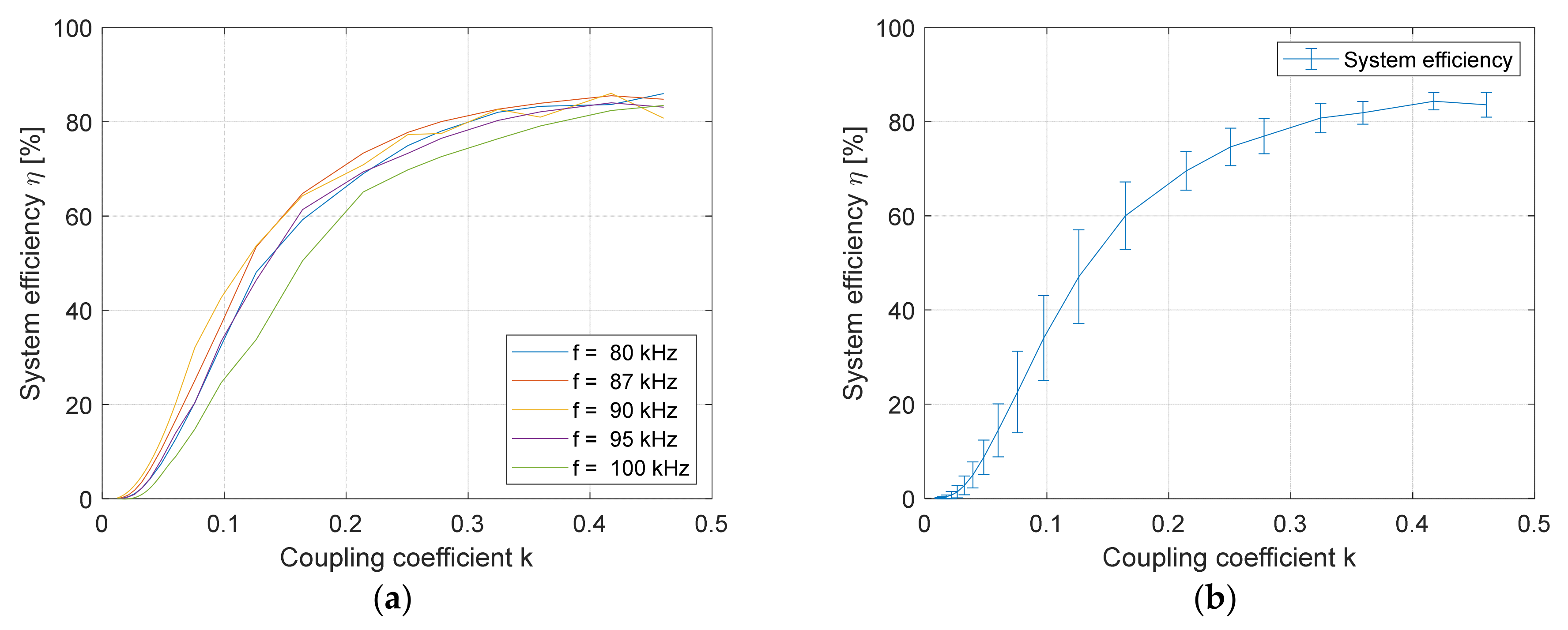
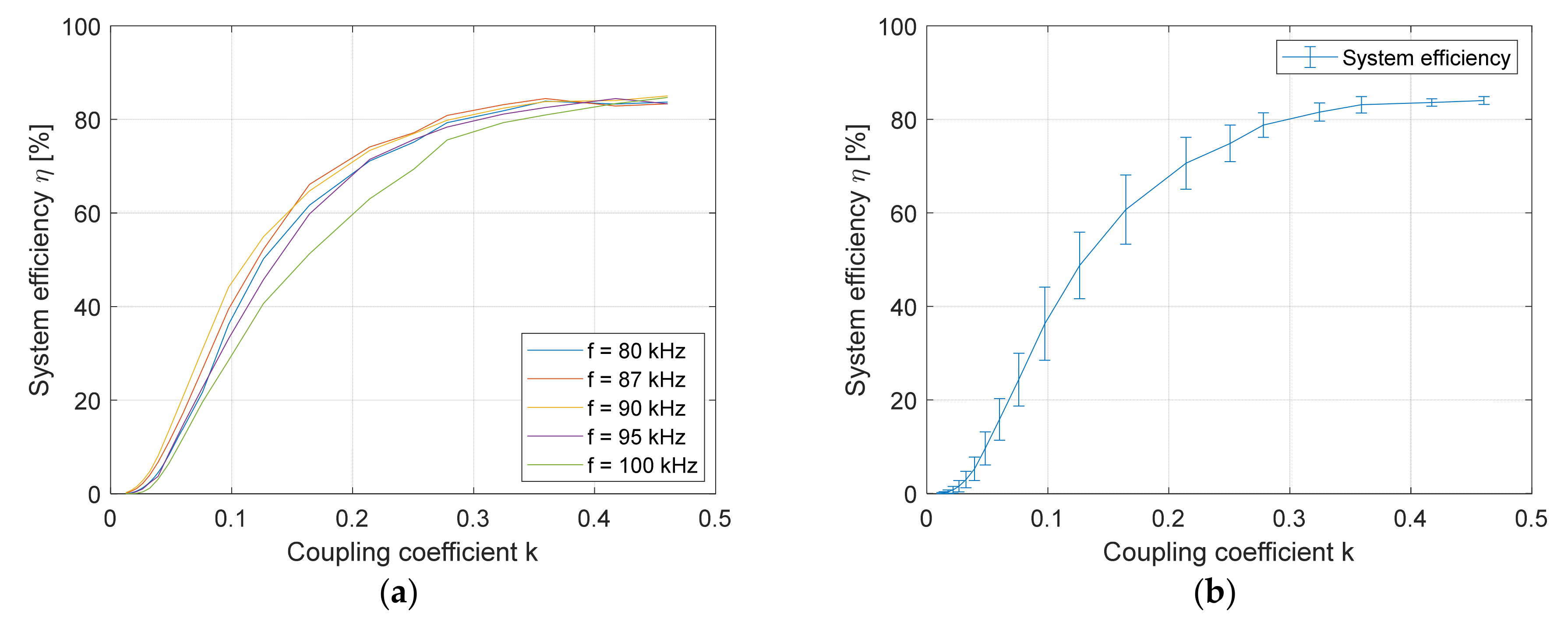
The efficiency of the single DD system is presented in the graph in Figure 16a,b. The efficiency of the double DD system is presented in the graph in Figure 17a,b. There was a small difference in efficiency between the operating points of the systems. The highest efficiency was around 84%. The different resonant frequencies do not show a significant impact on efficiency. Overall, at 90 kHz, both systems showed the best efficiency during the entire distance interval. When further increasing the frequency to 95 kHz and 100 kHz, the efficiency of both IPT systems decreased. In both cases, the efficiency was lowest when the transmitter coils were excited at 100 kHz. Figure 16b or Figure 17b present the average system efficiency and the maximum deviation from the average efficiency of the single DD and double DD IPT systems, respectively. In both cases, the largest deviation occurred under coupling coefficient 0.2.

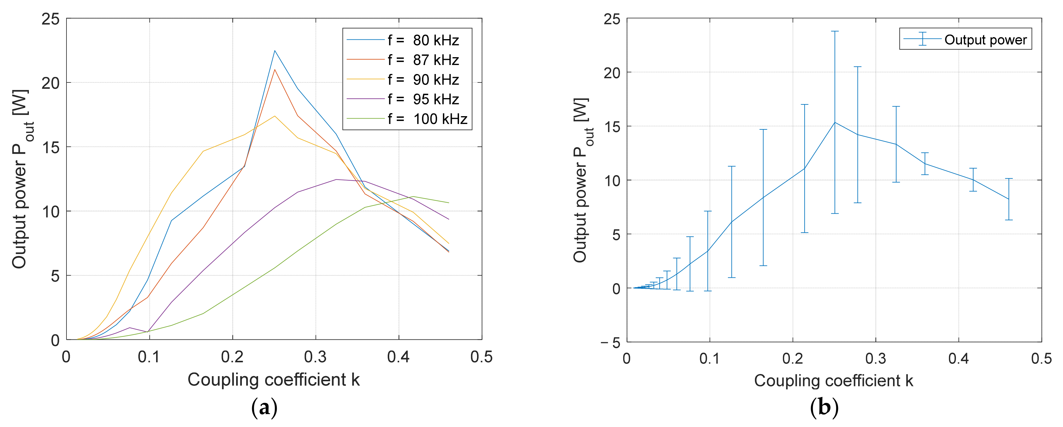
The output power capability of the single DD system is presented in Figure 18a,b. The output power capability of the double DD system is presented in Figure 19a,b. The average power output of both systems is presented in Figure 18b and Figure 19b for the single DD IPT and double DD IPT systems, respectively. In both cases, the deviation from average output power was significantly larger compared to the deviation from the average system efficiency in Figure 16b and Figure 17b. The capability of the double DD system is presented in Figure 19a,b. In the case of the double DD system, the input current was limited to 2 A DC. The double DD system had higher transfer power compared to the single DD system. The highest power transfer capability of the double DD system was around 36.4 W at 90 kHz. At the same frequency and distance, the single DD system transferred 17.4 W, around half as much. The output power of both systems decreased significantly at 95 kHz and 100 kHz.

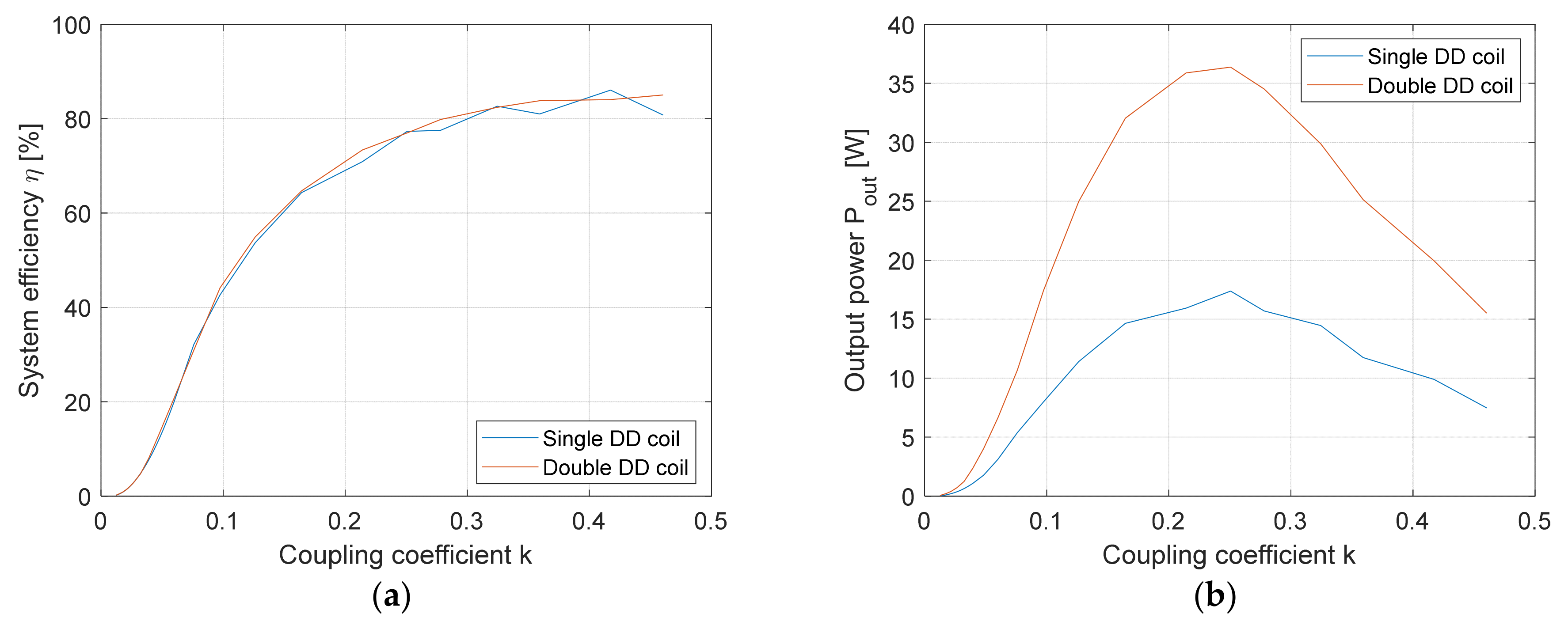
To evaluate the performance of the double DD system further, a direct comparison between the efficiency and output power is presented in Figure 20 and Figure 21. The results in Figure 20 are at the frequency of 87 kHz, and the results in Figure 21 are at the frequency of 90 kHz. Both the single DD and double DD IPT systems had remarkably similar efficiency. The biggest difference was in the transmitted power at the output of the system. Because the IPT system with double DD transmits power using two, uncoupled and independent coils, it can transfer twice as much power as the single DD system. Therefore, the double DD IPT system is the most attractive for wireless power transfer.

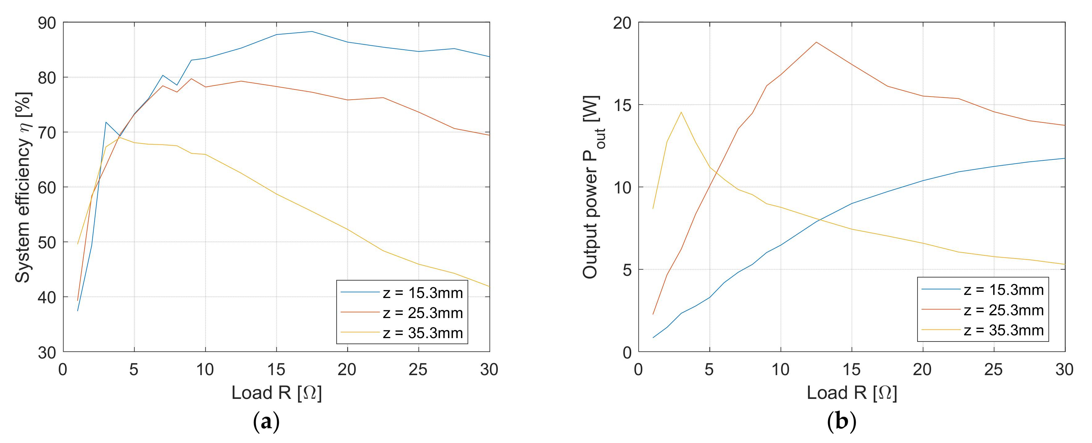
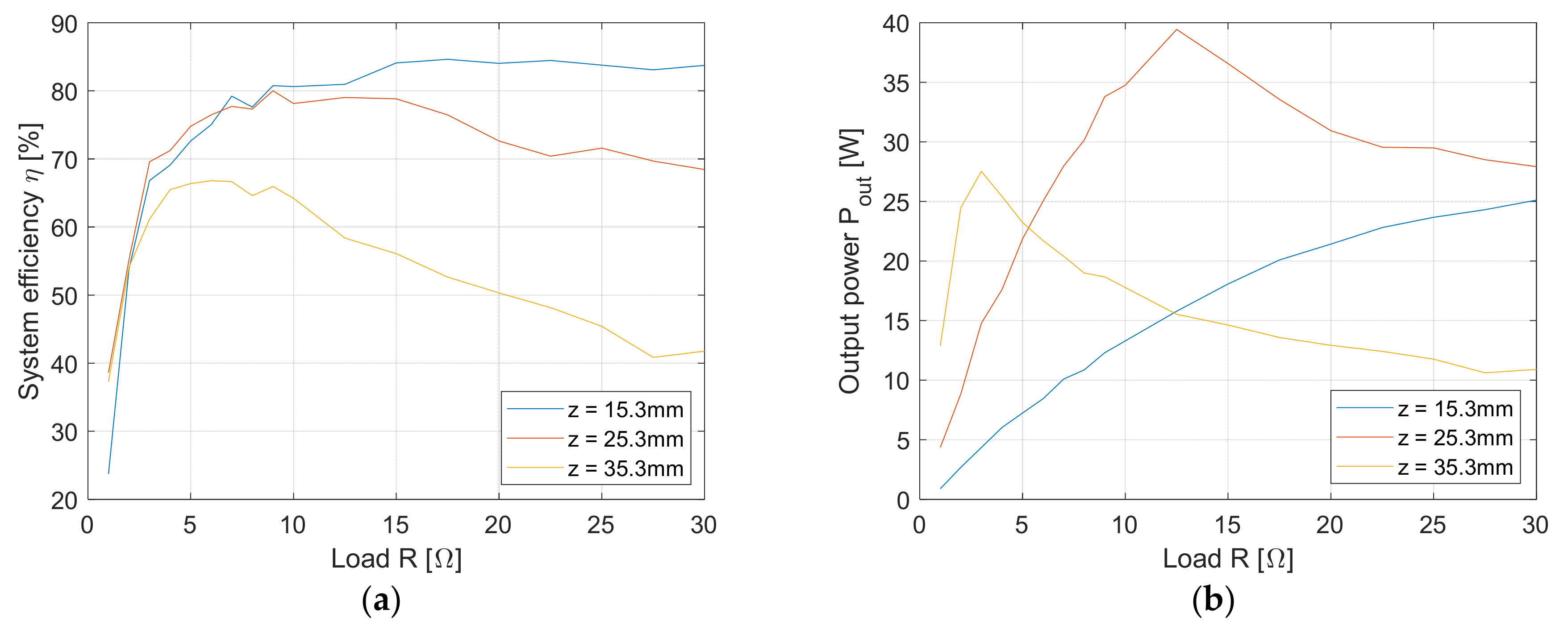
System efficiency and output power when load changed were also measured for both IPT structures at three different distances: at 15.3 mm, 25.3 mm, and 35.3 mm. The operating frequency was set to 87 kHz. The load was varied between 1 Ω and 30 Ω. The results of load variation in the case of the single DD IPT system are given in

Table 8. Single DD IPT system at different loads.

z (mm)	R (Ω)	UDC (V)	IDC (A)	Uout (V)	Pout (W)	η (%)
15.3	30	25.05	0.56	18.58	11.74	83.70
	25	25.05	0.53	16.56	11.24	84.65
	20	25.05	0.48	14.23	10.38	86.36
	15	25	0.41	11.42	8.99	87.75
	10	25	0.31	7.96	6.47	83.43
	8	25	0.27	6.471	5.30	78.53
	6	25	0.22	4.884	4.18	76.09
	4	25	0.16	3.245	2.77	69.28
	$⋮$	$⋮$	$⋮$	$⋮$	$⋮$	$⋮$
25.3	30	20.4	0.97	20.06	13.73	69.41
	25	20.6	0.96	18.81	14.56	73.63
	20	21.3	0.96	17.39	15.51	75.84
	15	23.2	0.96	15.90	17.44	78.28
	10	25	0.86	12.77	16.81	78.19
	8	25	0.75	10.63	14.49	77.26
	6	25	0.62	8.26	11.76	75.89
	4	25	0.48	5.63	8.35	69.61
	$⋮$	$⋮$	$⋮$	$⋮$	$⋮$	$⋮$
35.3	30	13.05	0.97	12.46	5.30	41.86
	25	12.95	0.97	11.84	5.77	45.93
	20	12.85	0.98	11.33	6.58	52.28
	15	13.05	0.97	10.38	7.43	58.70
	10	13.85	0.96	9.22	8.76	65.91
	8	14.7	0.96	8.62	9.53	67.50
	6	16.25	0.95	7.79	10.46	67.78
	4	19.4	0.95	6.95	12.71	68.97
	$⋮$	$⋮$	$⋮$	$⋮$	$⋮$	$⋮$

. The results of load variation in the case of the double DD IPT system are given in

Table 9. Double DD IPT system at different loads.

z (mm)	R (Ω)	UDC (V)	IDC (A)	Uout1 (V)	Uout2 (V)	Pout (W)	η (%)
15.3	30	25	1.2	19.65	18.74	25.12	83.74
	25	25	1.13	17.35	16.59	23.67	83.78
	20	25	1.02	14.79	14.11	21.43	84.03
	15	25	0.86	11.73	11.16	18.08	84.09
	10	25	0.66	8.26	7.84	13.31	80.64
	8	25	0.56	6.7	6.35	10.87	77.61
	6	25	0.45	5.073	4.78	8.44	75.04
	4	25	0.35	3.64	3.12	6.05	69.09
	$⋮$	$⋮$	$⋮$	$⋮$	$⋮$	$⋮$	$⋮$
25.3	30	20.4	2	19.79	20.69	27.93	68.45
	25	20.6	2	18.57	19.32	29.49	71.57
	20	21.3	2	17.37	17.71	30.95	72.64
	15	23.2	2	16.67	15.89	36.58	78.83
	10	25	1.78	13.53	12.48	34.77	78.12
	8	25	1.56	11.33	10.40	30.15	77.30
	6	25	1.31	8.98	7.97	25.05	76.48
	4	25	0.99	6.197	5.35	17.63	71.23
	$⋮$	$⋮$	$⋮$	$⋮$	$⋮$	$⋮$	$⋮$
35.3	30	13.05	2	12	13.27	10.90	41.78
	25	12.95	2	11.43	12.48	11.76	45.40
	20	12.85	2	10.67	11.76	12.93	50.31
	15	13.05	2	9.79	10.79	14.64	56.09
	10	13.85	2	9.41	9.21	17.78	64.20
	8	14.7	2	8.86	8.40	19.00	64.61
	6	16.25	2	8.28	7.51	21.72	66.82
	4	19.4	2	7.42	6.44	25.42	65.51
	$⋮$	$⋮$	$⋮$	$⋮$	$⋮$	$⋮$	$⋮$

. The tables include measured data at three different z distances.

The result that shows the impact of resistance on a single DD IPT system efficiency is shown in Figure 22a, and the impact of resistance on output power is shown in Figure 22b. Similarly, the results that show the impact of the resistance on the double DD IPT system are shown in Figure 23a,b.

The efficiency of the single DD IPT system was the same as the efficiency of the double DD IPT system, such was the case at the fixed load. In the case of both systems, lowering the resistance under 6 Ω also decreased system efficiency and transferred power. At a distance of 15.3 mm, the increment of the load did not affect the overall system efficiency negatively and only increased the transferred power. At distances of 25.3 mm and 35.3 mm, in both systems, the increment of load lowered the system efficiency, and it also lowered the amount of transferred power. At every load condition, the double DD IPT system transferred twice as much power as the single DD IPT.

5.7. The Impact of Horizontal Misalignment on the Transferred Power and the System Efficiency

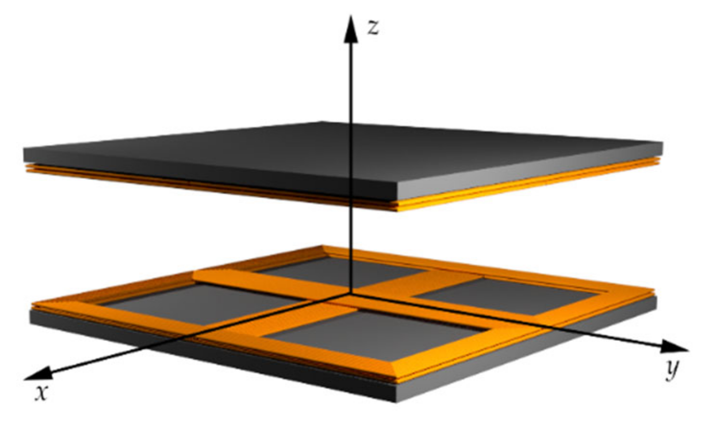
The main advantage of the DD coils is their great tolerance for misalignment. However, this only applies along one of the directions determined by the orientation of the DD coil. That means that the misalignment tolerance of the single DD coil is not symmetrical, which can be seen in the coupling coefficient evaluation, and was also confirmed with the following experiment. The position of the transfer pads in the 3D space is presented in Figure 24. The single DD power pad had a DD coil aligned with the DD1 coil in the x-axis direction. In the double DD coil system, the DD1 coil was aligned along the x-axis, and the DD2 coil was aligned along the y-axis. Both transmitter and receiver pad had the same orientation.

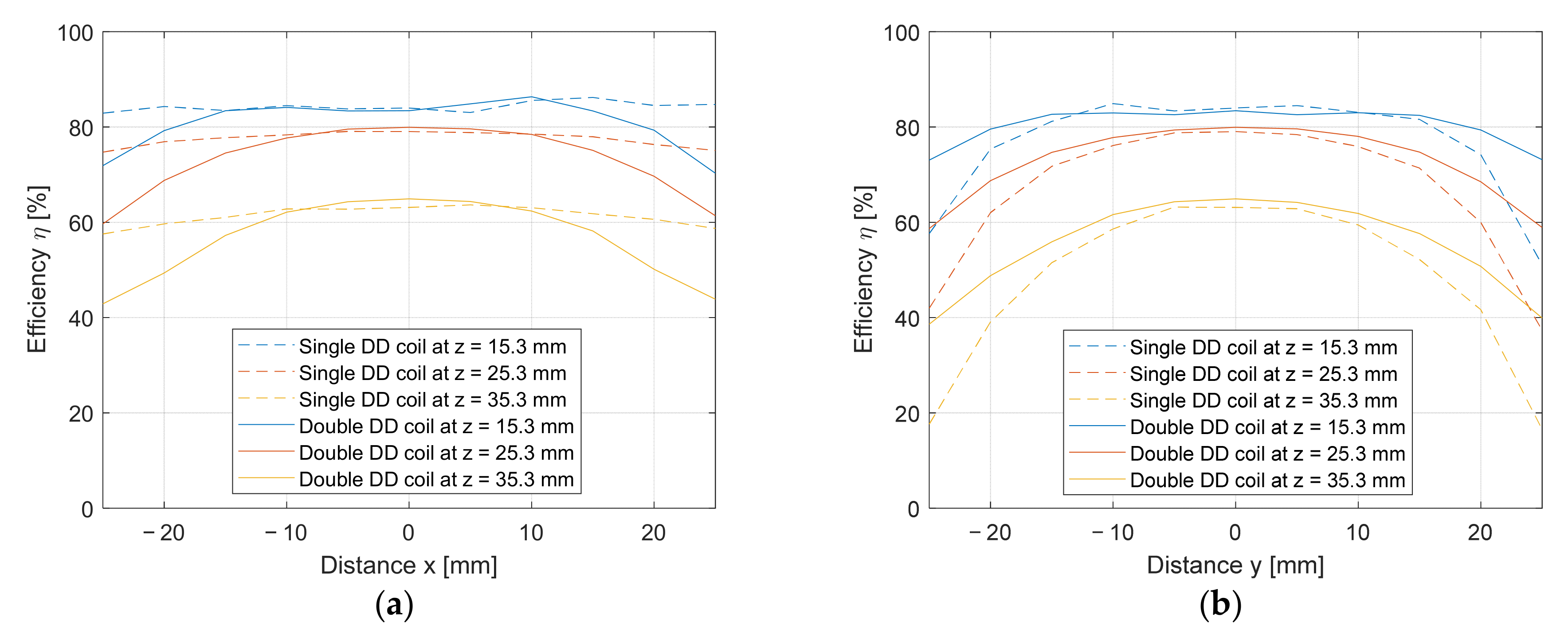
The single DD coil and double DD coil were misaligned horizontally from −25 mm to 25 mm in 5 mm steps along the x and y-axes. The measurements were performed at three different distances between the TX and RX pads: 15.3 mm, 25.3 mm, and 30.3 mm. The impacts of misalignment along the x-axis on the efficiency are presented in Figure 25a. The full lines stand for the results of the double DD coil system and the dashed lines are results for the single DD coil system.

The single DD coil was oriented in the x-direction, and was, therefore, tolerant for misalignment along the x-axis. The double DD coil consisted of a DD1 coil that was tolerant for misalignment along the x-axis and a DD2 coil that was not tolerant to misalignment along the x-axis. In the case of misalignment along the x-axis, the double DD coil system had lower efficiency compared to that of the single DD coil system. The difference in efficiency increased at larger misalignments.

On the other hand, the double DD coil system performed better than the single DD coil system in the case of misalignment along the y-axis, as presented in Figure 25b. The full lines are the results of the double DD coil system and the dashed lines stand for the results of the single DD coil system. Due to the poorer misalignment tolerance of the single DD coil along the y-axis, the efficiency of the system was also affected quite drastically. Because the double DD coil consisted of the DD1 coil that was not tolerant to misalignment along the y-axis and the DD2 coil that was tolerant, the resulting efficiency was higher compared to the single DD coil system. Therefore, the double DD coil had better misalignment tolerance than the single DD coil system in the y-direction. Overall, the double DD coil had the same symmetric misalignment tolerance along both the x and the y-axes. On the other hand, the single DD coil system did not have symmetric misalignment tolerance, and its tolerance was much better along the x-axis than along the y-axis.

Horizontal misalignment also had an impact on the transferred power. The comparison between transferred power using the single and double DD coils is presented in Figure 26a,b. The power transferred using the double DD coil system is represented by the full lines, and the power transferred using the single DD coil system is represented by the dashed lines.

Figure 26a shows the impact of horizontal misalignment along the x-axis, and Figure 26b shows the impact of the misalignment along the y-axis. Due to its structure, the double DD coil system has symmetrical power transfer when compared to the single DD coil system. Overall, the power transferred with the double DD coil system was larger when compared to the single DD coil system, even along the x-axis, when the single DD coil system had better efficiency.

6. Discussion

The results show that the double DD coupler structure enables higher power density compared to the single DD coupler. Each coil of the double DD system can transfer as much power as the system with the single DD coil. The IPT system with the double DD does not have overall better system efficiency when compared to the single DD system. System efficiency is determined by the transfer frequency and physical properties of the transfer pads, and the coupling coefficient between the transfer pads. Because both single and double DD structures used the same basic coil shape with the same dimensions and inductances, the impact of distance z on system efficiency was the same. The difference in efficiency between the single and double DD systems can be seen in the horizontal x-y plane misalignment. The proposed double DD coupler structure shows symmetrical tolerance to misalignment on the x-y plane. On the other hand, the misalignment of the single DD coil was not symmetrical. In the case of the misalignment along the x-axis, the single DD coil system performed better than the double DD coil system. In the y-axis, the double DD coil system had better efficiency than the single DD coil system. Nonetheless, the double DD coil system enabled higher power density when compared to the single DD coil system, and is, therefore, more attractive for applications where the space is limited.

7. Conclusions

This paper presents a double DD IPT coupler structure that can be used instead of a single circular nonpolar coupler or a polar DD coupler. The proposed coupler structure consists of two DD coils stacked on top of each other and perpendicular (rotated 90°) to each other. Because both coils are polarized and rotated, the DD coils on the pad are uncoupled magnetically. Therefore, both coils on a pad can transfer power independently of each other if the transfer pads are positioned correctly to each other. The coupling coefficient between the proposed pad structure was measured and compared to the coupling coefficient between single DD transfer pads. The double DD pads showed two separated coupling coefficients with different horizontal x-y plane tolerance and the same z-axis (distance) tolerance. To evaluate transferred power using the proposed pads, a double rectifier structure was used to transfer power to the same load in the same coil footprint and at the same time. This resulted in a 50% power transfer increase when compared to the single DD coil system at the same input voltage. The efficiency when increasing the z distance between the transfer pads in the case of the double DD coil system was similar to the single DD coil system. The maximum DC-DC system efficiency was between 80% and 85%, which also matches the simulation results. The DC–DC efficiency at coupling coefficients lower than 0.5 can be increased by using coils with larger inductance. At the operating point, the current state-of-the-art wireless charging systems have DC–DC efficiency from 80% to 90% and coil efficiency higher than 90%.

The double DD coil structure also showed symmetrical misalignment tolerance on the x-y plane compared to the non-symmetrical misalignment tolerance of the single DD coil.

References

1. Manoufali, M.; Bialkowski, K.; Mohammed, B.; Abbosh, A. Wireless Power Link Based on Inductive Coupling for Brain Implantable Medical Devices. IEEE Antennas Wirel. Propag. Lett. 2017, 17, 160–163. [Google Scholar] [CrossRef]
2. Jang, Y.; Jovanovic, M.M. A Contactless Electrical Energy Transmission System for Portable-telephone Battery Chargers. IEEE Trans. Ind. Electron. 2003, 50, 520–527. [Google Scholar] [CrossRef] [Green Version]
3. Triviño, A.; González-González, J.M.; Aguado, J.A. Wireless Power Transfer Technologies Applied to Electric Vehicles: A Review. Energies 2021, 14, 1547. [Google Scholar] [CrossRef]
4. Xiang, L.; Sun, Y.; Tang, C.; Dai, X.; Jiang, C. Design of Crossed DD Coil for Dynamic Wireless Charging of Electric Vehicles. In Proceedings of the 2017 IEEE PELS Workshop on Emerging Technologies: Wireless Power Transfer (WoW), Chongqing, China, 21–22 May 2017; IEEE: Piscataway, NJ, USA, 2017; pp. 1–5. [Google Scholar] [CrossRef]
5. Patil, D.; McDonough, M.K.; Miller, J.M.; Fahimi, B.; Balsara, P.T. Wireless Power Transfer for Vehicular Applications: Overview and Challenges. IEEE Trans. Transp. Electrif. 2017, 4, 3–37. [Google Scholar] [CrossRef]
6. Buja, G.; Bertoluzzo, M.; Mude, K.N. Design and Experimentation of WPT Charger for Electric City Car. IEEE Trans. Ind. Electron. 2015, 62, 7436–7447. [Google Scholar] [CrossRef]
7. Dai, J.; Ludois, D.C. A Survey of Wireless Power Transfer and a Critical Comparison of Inductive and Capacitive Coupling for Small Gap Applications. IEEE Trans. Power Electron. 2015, 30, 6017–6029. [Google Scholar] [CrossRef]
8. Jawad, A.M.; Nordin, R.; Gharghan, S.K.; Jawad, H.M.; Ismail, M. Opportunities and Challenges for Near-Field Wireless Power Transfer: A Review. Energies 2017, 10, 1022. [Google Scholar] [CrossRef]
9. SAE International J2954 Taskforce about Wireless Power Transfer for Light-Duty Plug-in/Electric Vehicles and Alignment Methodology. Available online: https://www.sae.org/standards/content/j2954_202010/ (accessed on 2 July 2021).
10. Wei, Z.; Quan, Z.; Wu, J.; Li, Y.; Pou, J.; Zhong, H. Deep Deterministic Policy Gradient-DRL Enabled Multiphysics-Constrained Fast Charging of Lithium-Ion Battery. IEEE Trans. Ind. Electron. 2021. early access. [Google Scholar] [CrossRef]
11. Wei, Z.; Zhao, J.; Xiong, R.; Dong, G.; Pou, J.; Tseng, K.J. Online Estimation of Power Capacity with Noise Effect Attenuation for Lithium-Ion Battery. IEEE Trans. Ind. Electron. 2019, 66, 5724–5735. [Google Scholar] [CrossRef]
12. Budhia, M.; Covic, G.A.; Boys, J.T. Design and Optimization of Circular Magnetic Structures for Lumped Inductive Power Transfer Systems. IEEE Trans. Power Electron. 2011, 26, 3096–3108. [Google Scholar] [CrossRef]
13. Budhia, M.; Boys, J.T.; Covic, G.A.; Huang, C. Development of a Single-Sided Flux Magnetic Coupler for Electric Vehicle IPT Charging Systems. IEEE Trans. Ind. Electron. 2013, 60, 318–328. [Google Scholar] [CrossRef]
14. Budhia, M.; Covic, G.; Boys, J. A new IPT magnetic coupler for electric vehicle charging systems. In Proceedings of the IECON 2010—36th Annual Conference on IEEE Industrial Electronics Society, Glendale, AZ, USA, 7–10 November 2010; pp. 2487–2492. [Google Scholar] [CrossRef]
15. Bima, M.E.; Bhattacharya, I.; Neste, C.W.V. Experimental Evaluation of Layered DD Coil Structure in a Wireless Power Transfer System. IEEE Trans. Electromagn. Compat. 2020, 62, 1477–1484. [Google Scholar] [CrossRef]
16. Kan, T.; Lu, F.; Nguyen, T.P.; Mercier, P.; Mi, C.C. Integrated Coil Design for EV Wireless Charging Systems Using LCC Compensation Topology. IEEE Trans. Power Electron. 2018, 33, 9231–9241. [Google Scholar] [CrossRef]
17. Cheng, C.; Li, W.; Zhou, Z.; Deng, Z.; Mi, C. A Load-Independent Wireless Power Transfer System with Multiple Constant Voltage Outputs. IEEE Trans. Power Electron. 2020, 35, 3328–3331. [Google Scholar] [CrossRef]
18. Shevchenko, V.; Husev, O.; Strzelecki, R.; Pakhaliuk, B.; Poliakov, N.; Strzelecka, N. Compensation Topologies in IPT Systems: Standards, Requirements, Classification, Analysis, Comparison and Application. IEEE Access 2019, 7, 120559–120580. [Google Scholar] [CrossRef]
19. Okada, K.; Sekino, T. The Impedance Measurement Handbook; A Guide to Measurement Technology and Techniques, App. Note; 2016, Keysight Technologies, Santa Rosa, CA, USA, 3 August 2014, 5950–3000. Available online: https://www.keysight.com/zz/en/assets/7018-06840/application-notes/5950-3000.pdf (accessed on 2 July 2021).
20. Ayyanar, R.; Mohan, N. A Novel Full-bridge DC-DC Converter for Battery Charging Using Secondary-Side Control Combines Soft-Switching over the Full Load Range and Low Magnetics Requirement. In Proceedings of the APEC 2000. Fifteenth Annual IEEE Applied Power Electronics Conference and Exposition (Cat. No.00CH37058), New Orleans, LA, USA, 6–10 February 2000; Volume 1, pp. 340–346. [Google Scholar] [CrossRef]
21. Wenli, L.; Ying, M.; Danan, S.; Shaolin, W.; Zhigang, L. Design of a Soft Switched 8 kW Battery Charging Converter for 100% Low Floor Light Rail Vehicle. In Proceedings of the 2008 IEEE Vehicle Power and Propulsion Conference, Harbin, China, 3–5 September 2008; pp. 1–5. [Google Scholar] [CrossRef]
22. Huynh, P.S.; Ronanki, D.; Vincent, D.; Williamson, S.S. Overview and Comparative Assessment of Single-Phase Power Converter Topologies of Inductive Wireless Charging Systems. Energies 2020, 13, 2150. [Google Scholar] [CrossRef]
23. Alexander, K.C.; Sadiku, N.O.M. Magnetically Coupled Circuits. In Fundamentals of Electric Circuits, 3rd ed.; Isenberg, S., Ed.; McGraw-Hill Higher Education: New York, NY, USA, 2007; pp. 528–531. [Google Scholar]
Figure 1. Exploded transmission pad: (a) With single DD coil; (b) with double DD coils.
Electronics 10 02528 g001
Figure 2. Magnetic flux lines between the transmitter and the receiver pad: (a) with single DD coil structure; (b) with double DD coil structure.
Electronics 10 02528 g002
Figure 3. (a) Conventional structure of a single DD coil; (b) proposed double DD coil structure.
Electronics 10 02528 g003
Figure 4. Block diagram of: (a) the coupling coefficient measurement system; (b) the IPT system.
Electronics 10 02528 g004
Figure 5. Circuit of a wireless power transfer system.
Electronics 10 02528 g005
Figure 6. Experimental set bench: (a) the coupling coefficent measurement set bench; (b) the IPT system set bench.
Electronics 10 02528 g006
Figure 7. Mutual inductances between transfer pads: (a) between pads’ coils on pads; (b) electrical scheme; (c) measurement of the inductance of a single DD coil; (d) measurement of the inductance between two DD coils.
Electronics 10 02528 g007aElectronics 10 02528 g007b
Figure 8. Mutual inductance measurement circuit: (a) measurement of coil inductance L′; (b) measurement of inductance LX1; (c) measurement of inductance LX2.
Electronics 10 02528 g008
Figure 9. Single DD x-y plane coupling coefficient measurements: (a) 15.3 mm distance between the pads; (b) 25.3 mm distance between the pads; (c) 35.3 mm distance between the pads.
Electronics 10 02528 g009
Figure 10. Double DD x-y plane coupling coefficient measurements: (a) 15.3 mm distance between the pads; (b) 25.3 mm distance between the pads; (c) 35.3 mm distance between the pads.
Electronics 10 02528 g010
Figure 11. Coupling coefficient measurement along the x-axis at z = 25.3 mm: (a) single DD coil; (b) double DD coil.
Electronics 10 02528 g011
Figure 12. Coupling coefficient measurement along the y-axis at z = 25.3 mm: (a) single DD coil; (b) double DD coil.
Electronics 10 02528 g012
Figure 13. Simulated magnetic flux density of the single and double DD coil structures: (a) magnetic flux density of the single DD in the x-z plane; (b) magnetic flux density of the single DD in the y-z plane; (c) magnetic flux density of the double DD in the x-z plane; (d) magnetic flux density of the double DD in the y-z plane; (e) magnetic flux density of the single DD in the x-y plane; (f) magnetic flux density of the double DD in the x-y plane.
Electronics 10 02528 g013aElectronics 10 02528 g013b
Figure 14. z-axis coupling coefficient measurement: (a) single DD coil stucture; (b) double DD coil structure.
Electronics 10 02528 g014
Figure 15. Comparison of the simulated and measured results: (a) single DD coil structure; (b) double DD coil structure.
Electronics 10 02528 g015
Figure 16. Efficiency of IPT using the single DD coil structure: (a) at different frequencies; (b) average system efficiency.
Electronics 10 02528 g016
Figure 17. Efficiency of the IPT using the double DD coil structure: (a) at different frequencies; (b) average system efficiency.
Electronics 10 02528 g017
Figure 18. Output power of the IPT using the single DD coil structure: (a) at different frequencies; (b) average output power.
Electronics 10 02528 g018
Figure 19. Output power of the IPT using the double DD coil structure: (a) at different frequencies; (b) average output power.
Electronics 10 02528 g019
Figure 20. Comparison between the single and double DD coil structures at the frequency 87 kHz: (a) system efficiency; (b) average output power.
Electronics 10 02528 g020
Figure 21. Comparison between the single and double DD coil structures at the frequency 90 kHz: (a) system efficiency; (b) average output power.
Electronics 10 02528 g021
Figure 22. Impact of load variation on the IPT with the single DD coil structure: (a) efficiency of the system; (b) output power transfer.
Electronics 10 02528 g022
Figure 23. Impact of load variation on the IPT with the double DD coil structure: (a) efficiency of the system; (b) output power transfer.
Electronics 10 02528 g023
Figure 24. Position of the IPT pads in the 3D space.
Electronics 10 02528 g024
Figure 25. Impact of horizontal misalignment on IPT system efficiency: (a) misalignment in the direction of the x-axis; (b) misalignment in the direction of the y-axis.
Electronics 10 02528 g025
Figure 26. Impact of the horizontal x misalignment on the IPT power output: (a) misalignment in the direction of the x-axis; (b) misalignment in the direction of the y-axis.
Electronics 10 02528 g026