Stability Analysis of Power Hardware-in-the-Loop Simulations for Grid Applications

Abstract

Power Hardware-in-the-Loop (PHiL) simulation is an emerging testing methodology of real hardware equipment within an emulated virtual environment. The closed loop interfacing between the Hardware under Test (HuT) and the Real Time Simulation (RTS) enables a realistic simulation but can also result in an unstable system. In addition to fundamentals in PHiL simulation and interfacing, this paper therefore provides a consistent and comprehensive study of PHiL stability. An analytic analysis is compared with a simulative approach and is supplemented by practical validations of the stability limits in PHiL simulation. Special focus is given on the differences between a switching and a linear amplifier as power interface (PI). Stability limits and the respective factors of influence (e.g., Feedback Current Filtering) are elaborated with a minimal example circuit with voltage-type Ideal Transformer Model (ITM) PHiL interface algorithm (IA). Finally, the findings are transferred to a real low-voltage grid PHiL application with residential load and photovoltaic system.

1. Introduction

A drastic reduction of greenhouse gas emissions in the energy sector requires a fundamental transition of energy supply [1]. The transformation of the electrical grid to integrate a vast amount of fluctuating renewable energy systems (RES) plays a key role on the way to a low-carbon society. However, this implicates new challenges for the existing energy system with the requirement of new market structures, closer communicative networking and new technological solutions [2]. The increasing complexity also demands for more comprehensive testing possibilities of new equipment [3,4]. The impact of the increasing penetration of the electrical energy system with power electronic converters requires more detailed modeling together with an in-depth consideration of converter control. Real Time Simulation (RTS), and Power Hardware-in-the-Loop (PHiL) in particular, will therefore play an increasing role in the validation and testing process of new systems and equipment in order to fully investigate its behavior in a flexible and realistic environment [3].

In the last decade a lot of research on PHiL simulation has been performed. Among others, stability analysis of a PHiL simulation at a theoretical basis is shown in [3,5,6,7,8,9,10,11,12,13] however, Refs. [7,10,11] solely focus on real impedance. In [6] complex impedances are also considered together with experimental validations, although without a quantitative analysis of the stability limits. Experimental validations of PHiL stability criteria with a linear power amplifier as power interface (PI) are shown in [6,10,14] whereas switching inverters are applied in [11,15]. However, to the knowledge of the author, no work has been done that explicitly applies PHiL stability theory to directly compare linear and switching inverters with the same real-time model and hardware setup.

Therefore, the focus of this paper is a consistent analysis of PHiL stability from theoretical considerations over a simulative approach to practical validations investigating the stability limit. Due to the fact that both switching and linear inverters are common in different laboratories, but behave differently, stability is shown for both converter types.

In the context of this research, the following work is done:

• A general analysis of PHiL stability based on the transfer function of a simplified circuit. The influence of impedance ratio, time delay, amplifier characteristics and low-pass filtering has been considered.
• An offline model of an exemplary PHiL simulation case was implemented in MATLAB Simulink™. Applying the findings of the theoretical analysis, the limits of stable PHiL simulation have been systematically investigated. Both, interfacing with a switching and a linear amplifier has been analyzed with a modeling approach.
• The modeling approach is validated with a real PHiL laboratory setup with both a linear and a switching amplifier in comparison.
• The results are applied to the example of a PV system with a residential load at the low-voltage grid to ensure stability in a real PHiL application.

Alongside with the analytic, simulative and experimental stability analysis, a brief introduction on the basic idea of RTS and the fundamentals of PHiL simulation techniques are explained in Section 2 as well as a presentation of the laboratory structures used in this work. The rest of the paper is structured as follows: In Section 3 the influencing factors on the stability of a PHiL simulation are analyzed based on an analytic approach. The findings are transferred to a simulative PHiL model and are experimentally validated in Section 4 with respect to the differences between linear and switching PI. Section 5 presents mitigation of an unstable PHiL simulation at the example of a real application by applying the findings of the previous sections. The results of the stability analysis and the deviations between the theoretical and experimental results are discussed in Section 6. A detailed summery along with the key findings of the research work is given in Section 7.

2. Power Hardware-in-the-Loop Simulation of Electrical Energy Systems

Hardware-in-the-loop (HiL) simulation provides flexibility to a laboratory installation and the possibility of testing at an early stage of development in a realistic environment.

In that way, physical components can be virtually coupled to any suitable grid with the possibility of freely adapting grid parameters. Thus, the behavior of an equipment at abnormal grid conditions can be examined in detail with reproducible results. Grid impact of new control or protection algorithms at an early stage of development can be tested with real hardware. Furthermore, new equipment can be implemented as a real-time model before prototyping to test the behavior within a real grid in a cost-effective way in an early stage of development [16,17,18].

HiL simulation is used whenever a single component or a part of a larger system shall be investigated in a realistic environment, especially if a laboratory setup of the whole system is not possible due to economic or technical reasons. HiL can be divided in Power Hardware-in-the-loop (PHiL) and Control-Hardware-in-the-loop (CHiL). The latter describes the interfacing of a real physical controller, protection relay or software within a simulated environment, e.g., RTS of an electrical grid. The interfacing between the RTS and the device under test is established via low-voltage analog signals or network communication protocols [19,20].

PHiL in contrary integrates physical power equipment into a real-time model of an electrical grid, resp., parts of an electrical grid. Amplification of the RTS signals to provide sufficient voltage level and currents for operation of the hardware is needed. However, the setup of an accurate and stable PHiL simulation is not straightforward [3], which will be shown in the context of this paper.

Different abbreviations are customary for the real physical equipment. Device under Test (DuT) [8,21], Equipment under Test (EuT) [20] or Physical Power System (PPS) [18] are seldom used. In contrast, Hardware under Test (HuT), is most common [6,13,14,15,16,20,22,23,24,25], therefore this abbreviation will be used in this paper. The virtual part of the system which has to be modeled and simulated in real time will be referred to as Real Time Simulation (RTS) in the following.

2.1. Real Time Simulation

Through significant improvements in CPU performance in the last decades, real-time-simulators now provide the ability to calculate even large power systems within microseconds [26,27]. This enables electromagnetic transient (emt)-simulation in real time. A realistic representation of the dynamics of a system in the discrete time domain requires sufficiently small simulation time steps [22,27,28]. Thus, real time in this context means:

• The fixed simulation time step has to be small enough to resolve even transients with sufficient accuracy;
• All calculations for a simulation time step, as well as the signal input and output, must be completed within the time period corresponding to the real time.

RTS is used whenever there is an interaction between a system operating at real-world speed and a model. With an offline simulation the computation time will rise with increased complexity of the model. Thus, a specific period of time in an offline simulation can be slower or faster than real-world time. Offline simulation programs often use variable time steps to increase accuracy around fast changing events or discontinuities [29]. However, digital RTS rely on fixed time steps. Each time step has to be solved during the time span that equals the real-world time which requires powerful processors [26].

Established RTS processors can simulate with time steps in the range of micro to milliseconds, whereas FPGA based simulators achieve even sub-microsecond simulation time steps [4].

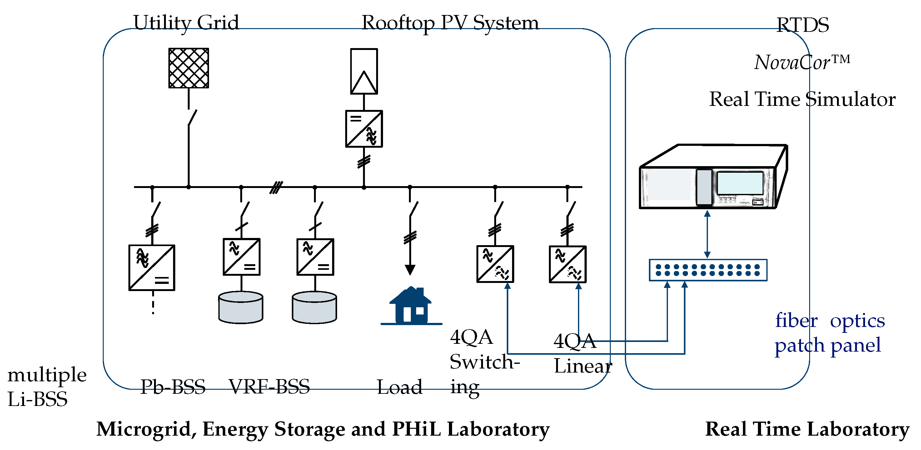
2.2. RTS-PHiL Laboratories

In the Real Time Laboratory, the Institute of Electrical Energy Systems (LEES) therefore controls multiple real-time simulators from different manufacturers. In this work a NovaCor™ simulator from RTDS Technologies Inc., Winnipeg, MB, Canada is used.

The Real Time Laboratory is coupled via optical fiber connections to the Microgrid, Energy Storage and Power Hardware-in-the-Loop Laboratory of the LEES. The laboratory is operated as a campus type microgrid with PHiL capabilities. The microgrid integrates battery storage systems (BSS) of different types, including a $15$ kWh/$5$ kVA vanadium-redox-flow storage system as well as a $4$ kWh/$4,6$ kVA lead-acid BSS and multiple lithium-ion based BSSs with a total of $82$ kWh. It is supplied by a rooftop photovoltaics (PV) system of $17.42$ kW rated power. A microgrid-controller for energy management is implemented on an industrial standard automation unit. Details can be extracted from [30,31]. Real-time digital simulators are not able to handle high voltage and currents. Therefore a power amplifier is required for interconnection of the RTS and the HuT. The laboratory is equipped with two three-phase four-quadrant amplifiers (4QA). A 4QA linear amplifier with a source and sink capability of $15$ kVA and a 4QA switching inverter with a nominal rated power of $45$ kVA with energy recovery capability. A schema of the laboratories is illustrated in Figure 1.

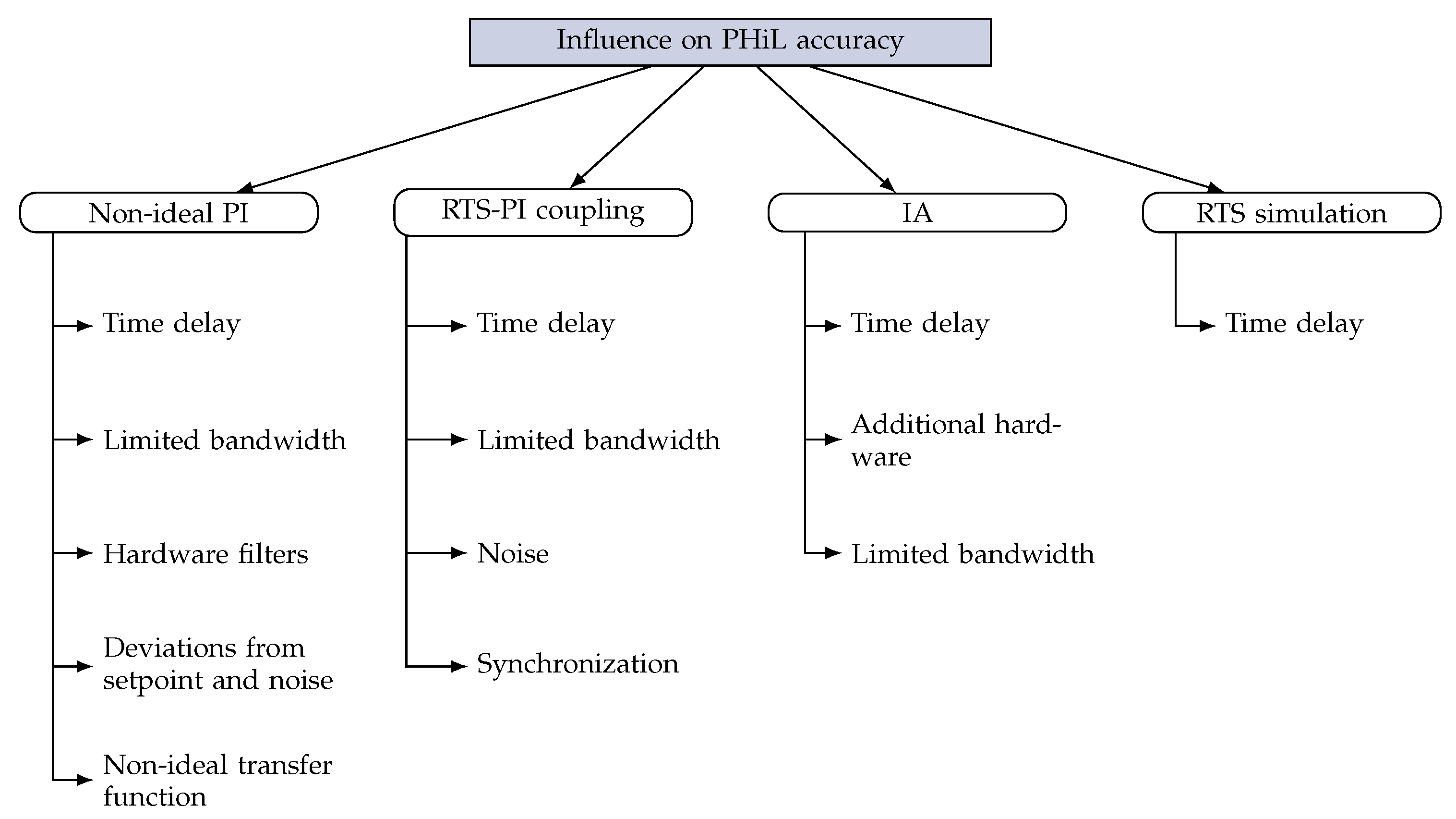
2.3. PHiL Simulation Fidelity and Errors

The division of an electrical grid into a simulated section and a hardware section implies the need for an interface. Inevitably, however, this will lead to a certain time delay between the two parts and to the introduction of noise into the system. These errors influence stability and accuracy of the PHiL simulation [3,15,19,23]. Figure 2 provides an overview of the effects that influence accuracy and therefore can result in stability issues.

The power interface provides non-ideal behavior, and thus introduces time delays, limited bandwidth, set-point deviations and measurement noise [5,32]. Eventually additional hardware is included in the circuit as inverter output filters. Another cause of error is the RTS itself which introduces a time delay through discrete time step simulation [5]. In addition the coupling between the RTS and the PI can introduce errors through communication time delays, limited bandwidth or through noise that is injected when using analog communication [5,32]. The PI and the RTS both operate at a specific sample time. If there is no time synchronization, variable delays occur which introduce harmonics and noise in the system [4] (see Section 3.2.3).

In addition, several IAs are known to improve PHiL stability [3]. However, IAs also introduce deviations from the ideal PHiL simulation by additional time delays, band limitation or extra hardware as stabilizing elements (see Section 2.6). Further details on accuracy with different IAs can be found in [3,5,8].

2.4. PHiL Power Interface

PHiL imposes the need for an amplifier as power interface (PI) to provide the voltage, resp., currents from the RTS at the HuT at an applicable level. In dependence on the application source and sink capability may be required. Four-quadrant operation of the PI is described as an independent control of positive and negative current and voltage and therefore an independent source and sink of real and reactive power [33].

A distinguishing feature of the PI is the converter technology that can be classified into switching and linear amplifiers. Linear amplifiers operate in the linear region of the semiconductors (e.g., linear-MOSFET), whereas switching converters are approaching the desired output voltage and current by high-frequency PWM which implicates the necessity of complex control loops and amplifier output filters [24].

The main advantages of linear amplifiers are small time delays and a wide frequency bandwidth [5,33,34]. The downside of linear amplifiers are high energy losses, up to one-third [33]. In comparison switching amplifiers provide efficiencies over $90\%$, are more economical and smaller in size [33,34]. However, a stable PHiL simulation may be more difficult to archive due to increased time delays and nonlinear behavior [5].

2.5. Communication between RTS and PI

The communication between the real time simulator and the PI is bidirectional. Interfacing can be implemented with analog signals or by digital communication protocols. For analog interfacing D/A and A/D converters are needed [11]. The induction of noise has to be prevented and galvanic isolation of simulator and PI is recommended [33]. Digital communication through fiber optics avoids noise and ground-loop problems and provides a fast broadband communication [33]. In this work the communication between the real time simulator and the amplifier is implemented with digital optical fiber AURORA communication protocol.

2.6. Interfacing Algorithms

Closed loop PHiL is characterized by mutual interaction between RTS and HuT. The interfacing therefore is crucial regarding stability and simulation accuracy [3]. With the IA it is specified, which values are being transmitted (e.g., voltage, current, power, torque, etc.) and how the signals are being processed (e.g., unity gain, low-pass-filtered, lead-lag compensator, etc.) [15].

The different IAs each have their own advantages and disadvantages. Therefore, a combination of different IAs is often used in order to achieve the best possible results [3]. The following section presents several different IAs and methods of enhancing the stability of a PHiL simulation.

2.6.1. Ideal Transformer Model (ITM)

The Ideal Transformer Model (ITM) algorithm (also called Ideal Transfer Model or Ideal Transformer Method [14,18]) is the most straightforward IA and very well established. It can be implemented as a voltage controlled variant or as a current controlled variant. For the voltage-type ITM, which is depicted in Figure 3, the reference voltage of the RTS is sent to the PI that forms the voltage at the HuT. This produces a current through the HuT which is measured and fed back to the RTS. For the current-type ITM the current of the RTS is amplified by the PI while the voltage across the HuT is used as feedback signal. The ITM IA offers high accuracy and has the benefit that no further hardware is needed. However, stability issues can be more challenging than in comparison with other interfacing algorithms [15].

2.6.2. Partial Circuit Duplication (PCD)

The PCD algorithm involves a linking component $Z_{ab}$, which is repeated in both RTS and the HuT, as illustrated in Figure 4. The larger the value of the linking impedance, the higher the stability of the system. However, with a higher value of $Z_{ab}$ the accuracy decreases due to increased power losses [15]. Note that feedback from the HuT is implemented by a controlled voltage source in the RTS. In [35] detailed discussion of the PCD algorithm is provided.

2.6.3. Damping Impedance Model (DIM)

The DIM algorithm consists of a combination of ITM and PCD techniques. It requires a linking impedance $Z_{ab}$ as well as a damping impedance $Z^{*}$. Its schematic is depicted in Figure 5. This method leads to absolutely stable results if $Z^{*}$ is equal to the impedance of the HuT $Z_{HuT}$. In reality, the knowledge of the exact value of $Z_{HuT}$ requires a perfect model of the HuT which is usually not available. Furthermore, it would make the PHiL simulation dispensable. Nevertheless, high stability margins and good accuracy can still be achieved with the DIM-Algorithm if $Z^{*}$ is close to the actual value of the hardware impedance [15].

2.6.4. Transmission Line Model (TLM)

The TLM algorithm involves a reactive linking component $Z_{lk}$, which is considered as a Bergeron transmission line section and modeled as an equivalent Norton or Thévenin circuit. This algorithm is commonly used for decoupling large systems with sufficiently long transmission lines for the benefit of parallel computation. It offers high stability given that it is numerically based on the trapezoidal approximation. However, it might lead to some drawbacks such as large power consumption, low flexibility and high maintenance cost [15,36].

2.6.5. Hardware Inductance Addition Method (HIA)

The HIA-method can be applied to voltage-type interfaces. It involves an additional inductance $L_{ADD}$, which is added to the hardware side. $L_{ADD}$ is connected in series with the HuT and leads to an improvement in stability but also to a decrease in accuracy [3].

2.6.6. Feedback Signal Filtering (FSF)

FSF applies a low-pass filter to the feedback signal. Figure 6 illustrates the Feedback Current Filtering Method (FCF) at the example of the voltage type ITM algorithm. The filter improves the stability of the system. It can be implemented analogue or in software. For this reason, further hardware is not necessarily needed. Its influence on the stability and accuracy of the simulation depends on the cut-off frequency of the filter [37]. FSF can also be combined with other IAs [3].

2.6.7. Further Interfacing Algorithms

Other possible interfacing algorithms are the Time-variant First-order Approximation (TFA) which is discussed in [15] and the Taganrog Algorithm. A description of the Taganrog Algorithm can be found in [35]. The Multi-Rate Partitioning Method (MRP) and the Partial Shifting Impedance (PSI) are—like HIA and FSF—further methods of improving the stability of a PHiL simulation. Ref. [3] presents an overview of these methods.

3. Analytic Approach to PHiL Stability

In this section the stability of a PHiL simulation is investigated analytically. To keep the analysis as comprehensible as possible a minimal example of a PHiL setup is introduced in Section 3.1. In Section 3.2 the stability of a PHiL simulation is analyzed by applying Nyquist stability criterion (NSC) to the open loop transfer function (OLTF). Subsequently the findings are compared with an emt simulation in MATLAB Simulink™ and an experimental setup in the following chapter (Section 4) to validate the analytic approach.

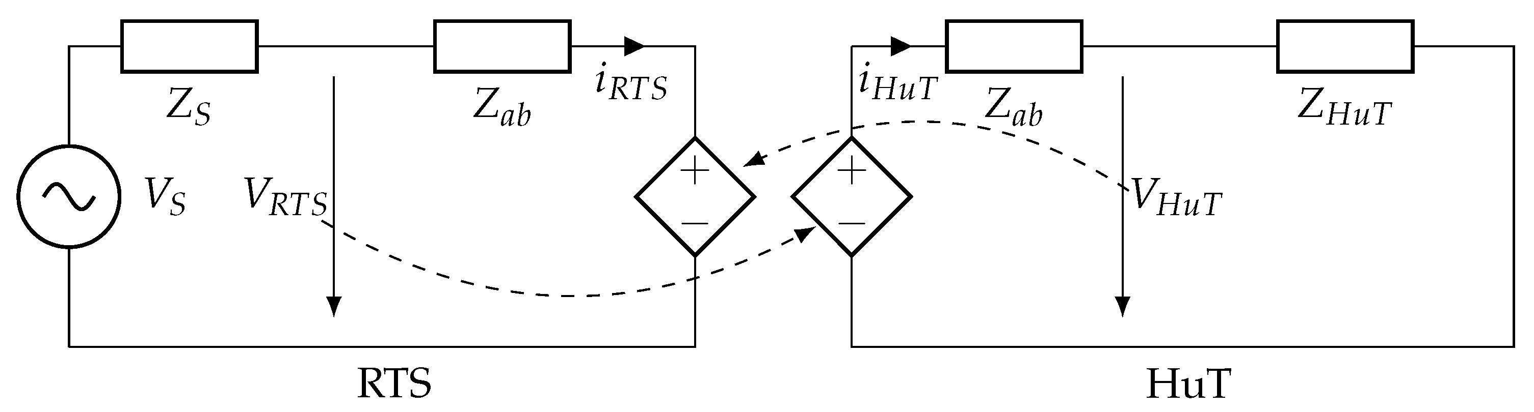
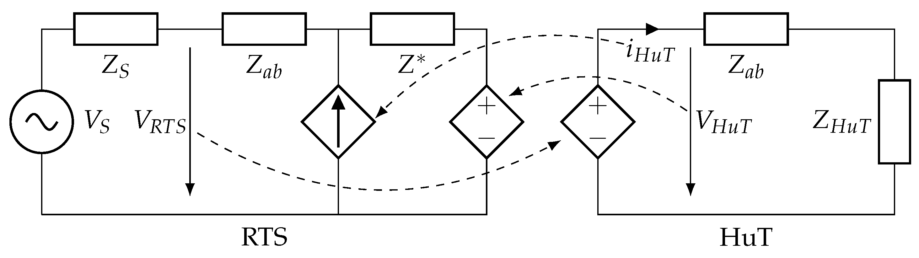
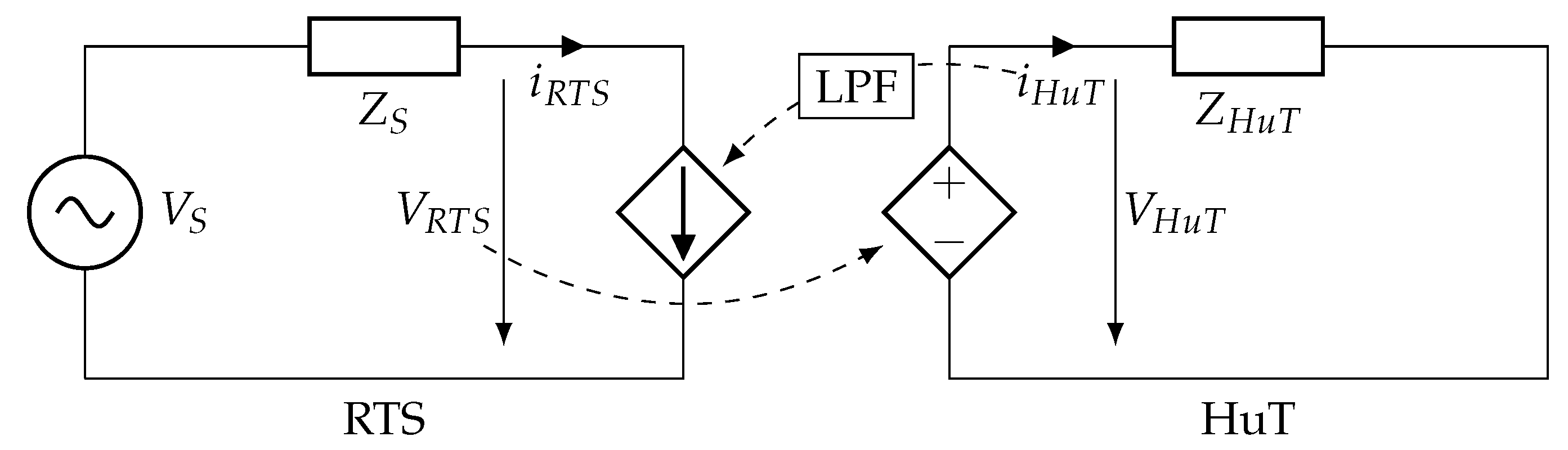
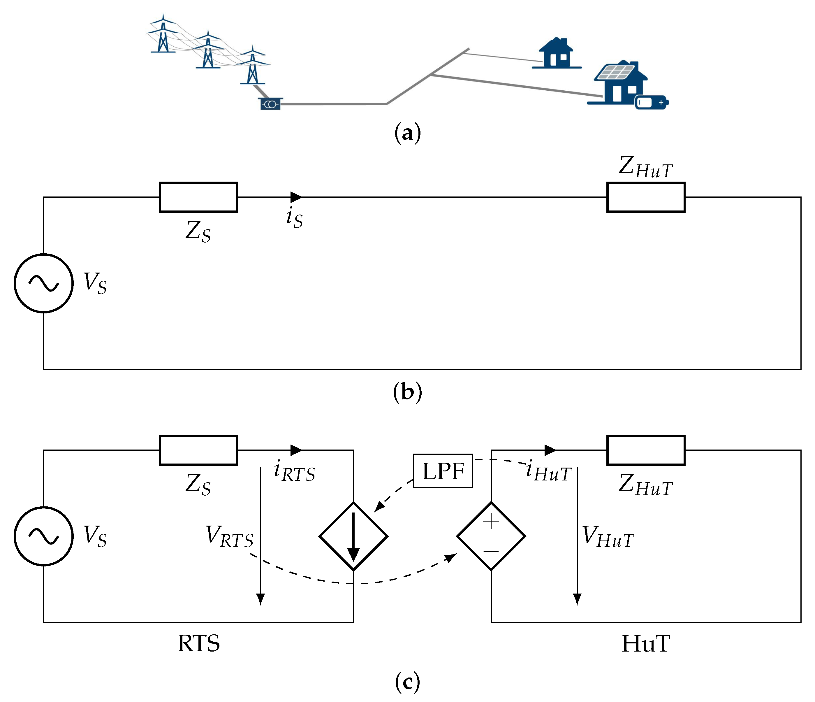
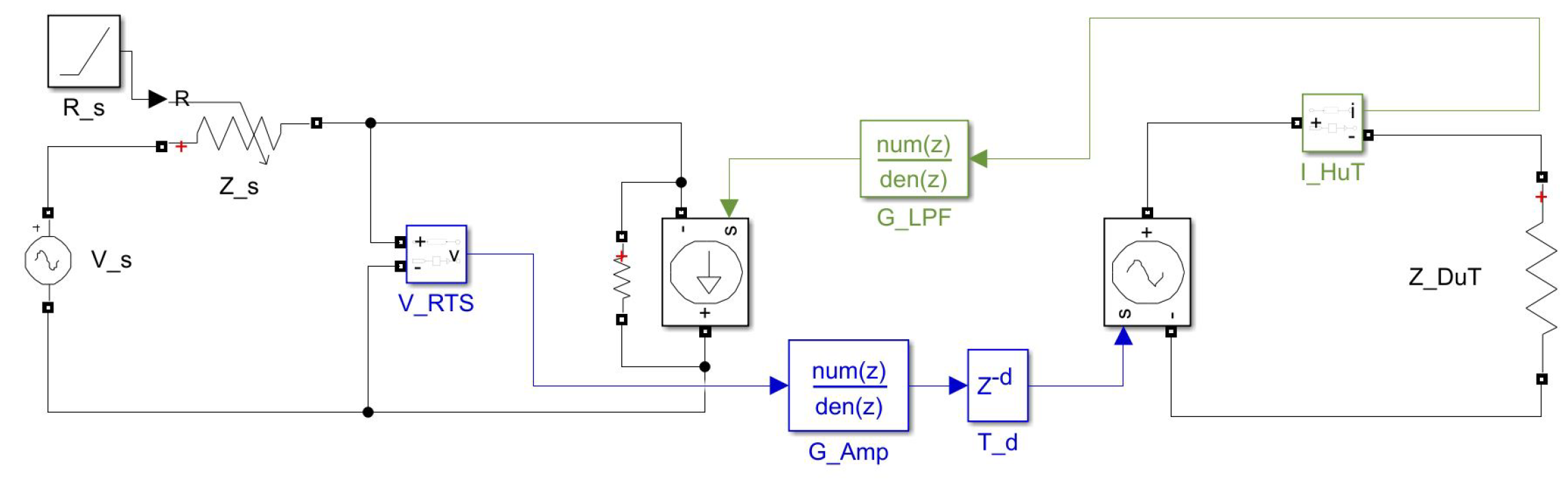
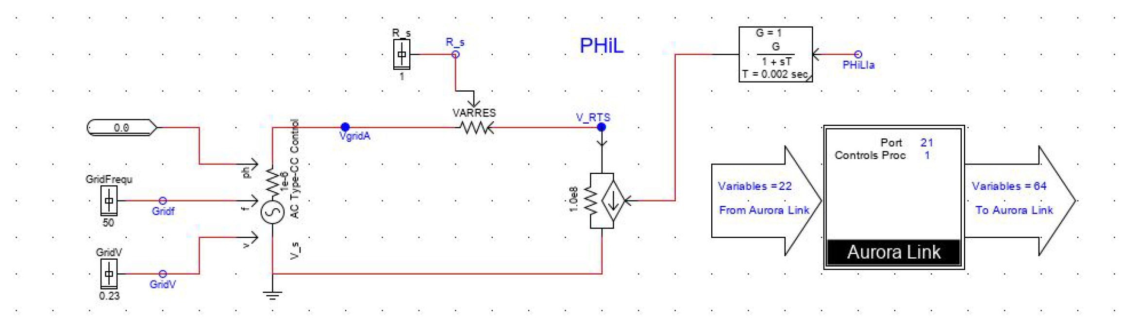
3.1. Minimal PHiL Example Circuit

To analyze the influencing parameters on PHiL stability an exemplary section of a low-voltage grid shall be reduced to a simple, single-phase circuit. An ideal voltage source $V_S$ with equivalent impedance $Z_S$ represents a low voltage distribution grid as depicted in Figure 7 and the impedance $Z_{HuT}$ represents a residential load.

The circuit in Figure 7 can be split into a virtual model and a physical part. An active HuT (e.g., a power electronics inverter or a generator supplying the grid) can be represented as an additional voltage or current source within the HuT, which is shown in [8,37]. In case the circuit includes nonlinearities, the following stability criterion is not applicable without simplification. This issue is addressed in [14,15]. For simplicity, the HuT is therefore considered as a passive, linear system in this work.

In general, the impedance on the RTS side $Z_S$ can be directly obtained from the model. However in most practical PHiL applications the impedance $Z_{HuT}$ of the HuT is not known exactly and is time dependent as well. In this case it can be calculated based on Ohm’s law, with a measurement of voltage and current and the $cos\left(\phi \right)$. In case of active and nonlinear load, however, this is far more complicated. Impedance estimation techniques have to be applied, which are described in [5,10].

Due to its simplicity, the PHiL coupling is implemented as voltage type ITM according to Figure 3. The circuit from Figure 7 can be considered as a voltage divider, which is generally known to be stable. However, the interfacing between RTS and HuT provides a time delay and non-ideal behavior which can result in instabilities [11].

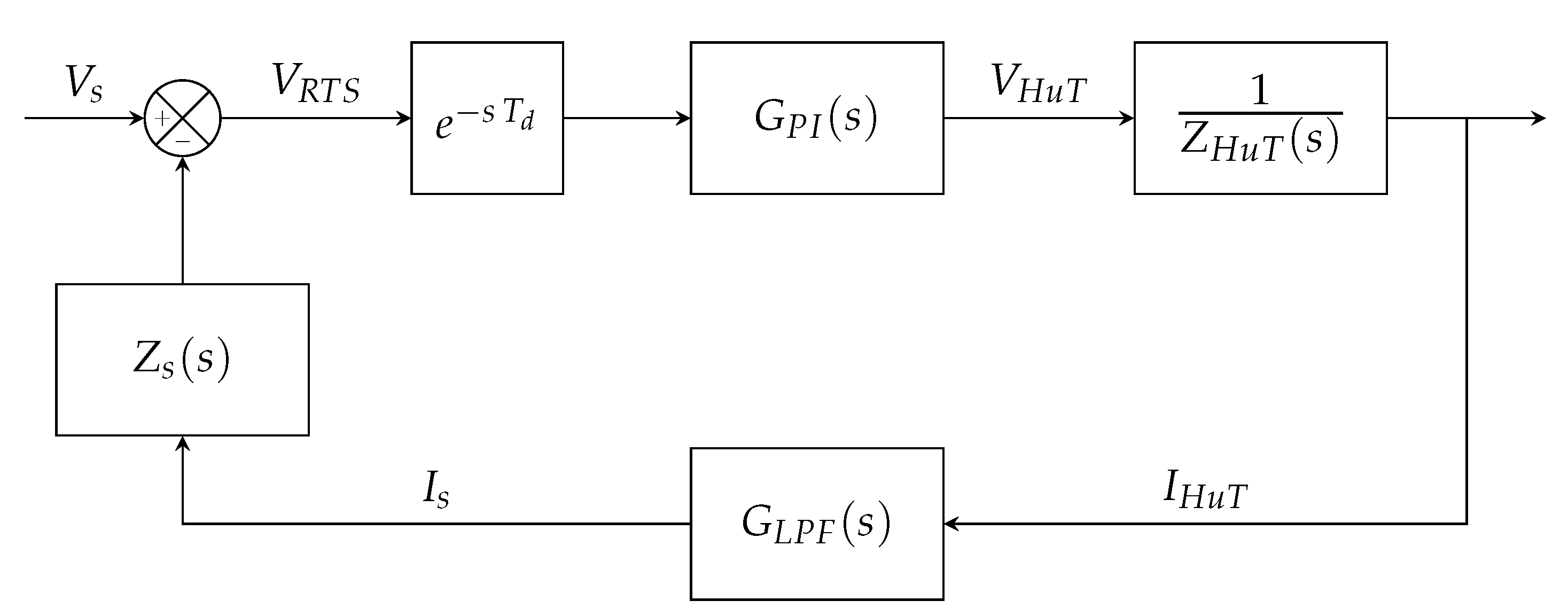
3.2. Analytic Stability Analysis

In this section stability of a PHiL simulation will be investigated analytically at the example of voltage type ITM. Therefore the transfer function of a PHiL circuit is analyzed with NSC. A brief introduction to NSC is provided in [6,38].

The voltage type ITM PHiL circuit from Figure 7 can be represented as a block diagram which is shown in Figure 8.

The block diagram is implemented in the s-plane. The equivalent grid voltage $V_S$ can be considered as the input of the control loop. All time delays (simulation, communication, amplifier, measurement, etc.) are summed up to a single loop delay time constant $T_d$. The transfer function $G_{PI}\left(s\right)$ of the PI connects to the voltage $V_{HuT}$ at the HuT. An optional low-pass filter $G_{LPF}\left(s\right)$ for FSF (see Section 3.2.4) is present in the current feedback path. The OLTF of the PHiL circuit is derived as the product of all blocks within the loop:

$$\begin{array}{c}\hfill G_{OLTF}\left(s\right)=G_{PI}\left(s\right)·G_{LPF}\left(s\right)·\frac{Z_S\left(s\right)}{Z_{HuT}\left(s\right)}{e}^{-s{T}_d}\end{array}$$

(1)

In [10] the representation of time delays in PHiL simulation as a polynomial transfer function for treating as an linear time-invariant system is given special focus. However, within the content of this work the exponential representation $e^{-s{T}_d}$ is sufficient due to the direct applicability in MATLAB™. In the following, stability of the PHiL circuit is analyzed on the basis of the transfer function $G_{OLTF}\left(s\right)$.

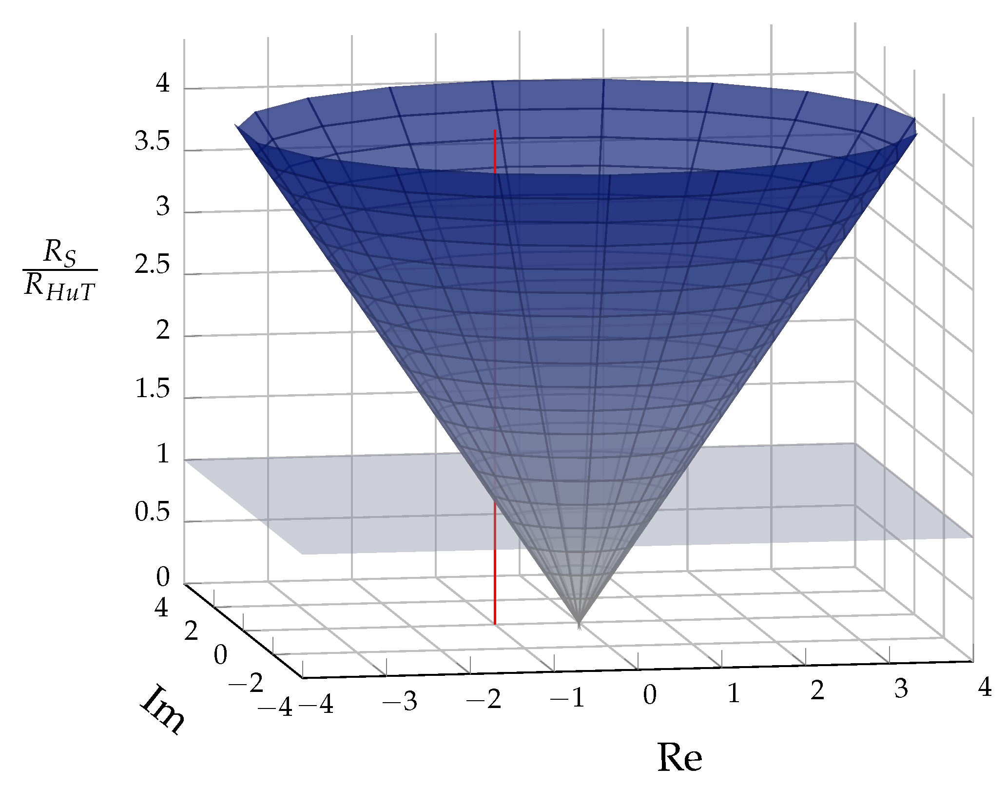
3.2.1. Resistive Impedance

The circuit in Figure 7 is assumed to be pure resistive with $Z_S$ and $Z_{HuT}$ having only a real component. For simplicity the influence of the amplifier $G_{PI}\left(s\right)$ is neglected in this section and FSF is not applied. The simplified OLTF can be rewritten as:

$$\begin{array}{c}\hfill G_{OLTF}\left(s\right)=\frac{R_S}{R_{HuT}}{e}^{-s{T}_d}\end{array}$$

(2)

The resistance $R_S$ and $R_{HuT}$ are assumed to be frequency independent. Figure 9 depicts a locus plot with the quotient of the resistance $R_S$ over $R_{HuT}$ as an additional dimension. With NSC stability margins can be analyzed. In simplified terms, NSC considers a system to be unstable if the Nyquist curve encloses the critical point $(-1,\mathrm{j}0)$ in the locus plot of the OLTF [6,7]. The Nyquist curve of the OLTF in Equation (2) describes a circle with radius $\frac{R_S}{R_{HuT}}$ around the origin. Figure 9 therefore forms a funnel-shaped surface. $(-1,\mathrm{j}0)$ is marked over the whole range of the impedance ratio as a red line within the figure. Thus, instability is indicated when the critical line intersects the surface. This is the case at a ratio of $\frac{R_S}{R_{HuT}}\ge 1$ (above the blue plane).

The loop delay $e^{-s{T}_d}$ is frequency dependent, but does not affect the magnitude of the signal. The Nyquist curve in Figure 9 forms a circle around the origin. Thus, a change in phase does not affect the radius of the cycle and therefore has no influence on stability [6]. Figure 10 shows that the radius is not changing, but the number of encirclements until a finite circular frequency.

3.2.2. Complex Impedance

The assumption of purely resistive impedances is a very special case. Therefore, in the following, a PHiL simulation with complex impedances $Z_S$ and $Z_{HuT}$ is analyzed.

The OLTF can be expressed as:

$$\begin{array}{c}\hfill G_{OLTF}\left(s\right)=\frac{R_S+s{L}_S}{R_{HuT}+s{L}_{HuT}}{e}^{-s{T}_d}\end{array}$$

(3)

Both resistances $R_S$ and $R_{HuT}$ and inductances $L_S$ and $L_{HuT}$ are assumed to be frequency independent.

In the frequency domain the OLTF can be rewritten as:

$$\begin{array}{c}\hfill G_{OLTF}\left(j\omega \right)=\frac{R_S+\left(j\omega \right)L_S}{R_{HuT}+\left(j\omega \right)L_{HuT}}{e}^{-\left(j\omega \right)T_d}\end{array}$$

(4)

With frequencies approaching close to zero ($\omega \to 0$), we obtain the previous example with resistive behavior, were the Nyquist curve describes a circle. The center of this circle is zero with a radius of $\frac{R_S}{R_{HuT}}$. Thus, the Nyquist curve starts at the positive real axis at the position $(\frac{R_S}{R_{HuT}},\mathrm{j}0)$.

If frequency, however, points towards infinity ($\omega \to \infty$), the fractional term $\frac{R_S+\left(j\omega \right)L_S}{R_{HuT}+\left(j\omega \right)L_{HuT}}$ approaches $\frac{L_S}{L_{HuT}}$ whereas the expression $e^{-\left(j\omega \right)T_d}$ forms an infinite rotation in mathematically positive direction. Therefore, the locus plot at $\omega \to \infty$ approaches a circle with radius $\frac{L_S}{L_{HuT}}$.

Consequently, both, the ratio of $\frac{R_S}{R_{HuT}}$ and $\frac{L_S}{L_{HuT}}$ have an influence on PHiL stability [6].

In dependence of the ratio of the impedances, three cases are distinguished in the following.

Case A:$R_S\le R_{HuT}$ and $L_S\le L_{HuT}$

As explained before the Nyquist curve starts in the point $(\frac{R_S}{R_{HuT}},j0)$ and ends on a circle with radius $\frac{L_S}{L_{HuT}}$. If both the starting and ending points of the locus curve are within the unit circle than the critical point at ($-1,j0$) is never enclosed [6]. According to the NSC this guarantees stability of the PHiL simulation and this is the case, if both, the ratio of $\frac{R_S}{R_{HuT}}\le 1$ and $\frac{L_S}{L_{HuT}}\le 1$.

Case B:$R_S\le R_{HuT}$ or $R_S>R_{HuT}$ and $L_S>L_{HuT}$

In case of $R_S\le R_{HuT}$ the Nyquist curve starts within the unit circle, respectively if $R_S>R_{HuT}$ the curve starts outside of the unit circle. Due to the ratio of $\frac{L_S}{L_{HuT}}>1$ the locus curve reaches a circle that encloses the critical point at ($-1,j0$) which makes Case B always unstable whenever $L_S>L_{HuT}$. In this case HIA (see Section 2.6.5) could be very efficient.

Case C:$R_S>R_{HuT}$ and $L_S\le L_{HuT}$

The locus curve starts outside the unit circle in this case, due to $\frac{R_S}{R_{HuT}}>1$, however, at high angular frequencies $\omega \to \infty$ it approaches a circle with radius $\frac{L_S}{L_{HuT}}\le 1$ which is inside the unit circle. Whether the critical point at ($-1,j0$) is enclosed by the Nyquist curve (which would make the PHiL simulation unstable), depends on the position of the first root in the left half plane, that is, were the curve intersects the negative real axis the first time [6]. If the first intersection point occurs within the unit circle, i.e., to the right of the critical point, all further intersection points are also within the unit circle. The critical point ($-1,j0$) is therefore never enclosed which results in a stable system. However, if the first intersection appears outside the unit circle, the PHiL is unstable. In [6] a formula is given to examine stability for Case C in dependence of the values of $R_S$, $R_{HuT}$, $L_S$ and $L_{HuT}$.

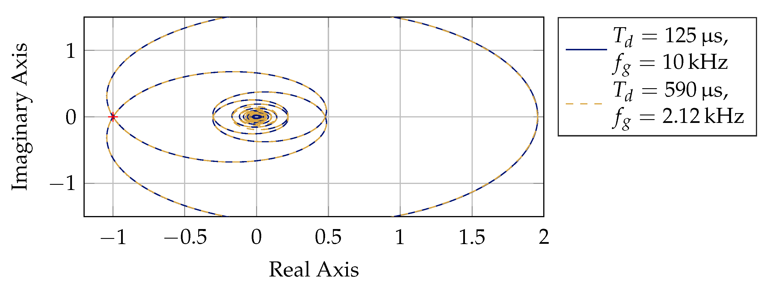
3.2.3. Influence of Time Delay

According to the previous sections, the time delay has no influence on stability within PHiL simulations regarding Case A and as long as the impedances are purely resistive. Even at a loop delay which equals a phase shift of ${180}^{\circ }$ in the fundamental frequency a stable PHiL simulation can be achieved [39].

However, regarding Case C in Section 3.2.2 time delay can be decisive whether the critical point ($-1,j0$) is enclosed by the Nyquist curve or not.

Apart from stability, time delay has an influence on PHiL simulation accuracy. In voltage type ITM the current in the RTS is determined by the loop-back signal from the measurement of the HuT current. A time delay in the PHiL loop therefore manifests itself as a phase shift between voltage and current in the RTS, which affects the power factor. The loop delay therefore reduces accuracy, since the phase shift results in a reactive power within the RTS which is not present in the HuT [4]. The power factor deviation through loop delay in dependence on system frequency $f_s$, loop delay $T_d$ and the real active and apparent power flow, that is simulated by the PHiL, can be calculated according to the following equation:

$$\begin{array}{c}\hfill cos{\phi }_{RTS}=cos\left(2\pi T_d{f}_s\right)\end{array}$$

(5)

In [4], the influence of variable time delays is investigated. Due to the interaction of multiple discrete time systems, a time delay of variable duration can occur, if the discrete systems are not synchronized. This results in an oscillation or noise in the loop-back signal [4].

Noise can be reduced by a low-pass filter (LPF), which commonly has a positive influence on PHiL stability [3].

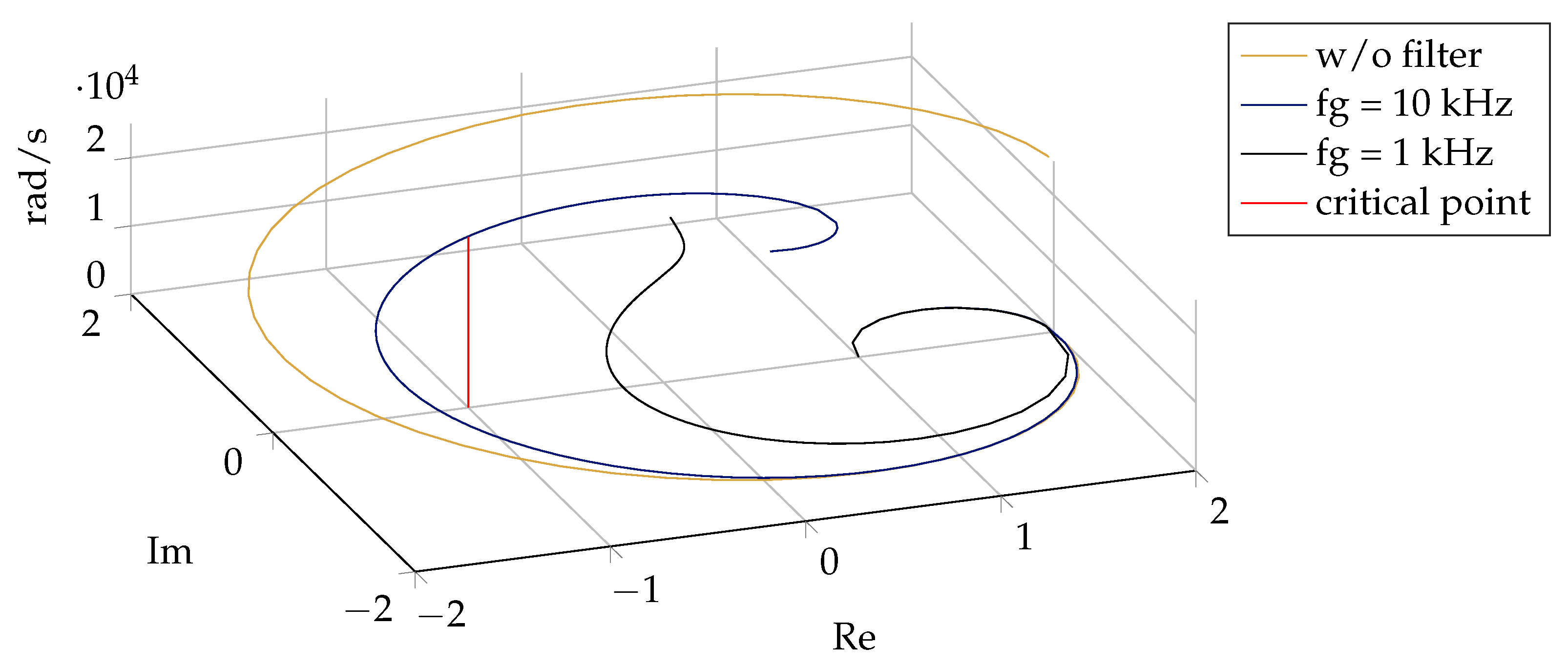
3.2.4. Stability Improvement with Feedback Signal Filtering

A limitation of the bandwidth of the PHiL loop reduces the accuracy but can have a stabilizing effect on the simulation [3]. A LPF can be implemented in software or in hardware. A software implementation in the feedback loop (see $G_{LPF}$ in Figure 7) makes it a flexible stability improvement with simple implementation without a need for additional hardware [3,23]. The transfer function, a first-order LPF in the s-plane, can be expressed as follows:

$$\begin{array}{c}\hfill G_{LPF}\left(s\right)=\frac{1}{(1+\frac{s}{2\pi f_g})}\end{array}$$

(6)

With complex frequency s and the cut-off frequency $f_g$.

Due to the damping of the amplitude of a signal at frequencies larger than $f_g$ the locus plot will approach the origin ($0,0$) at $\omega \to \infty$. Furthermore the phase is increased by the filter. Thus, with decreasing cut-off frequency $f_g$ the radius of the Nyquist curve decreases faster, which stabilizes the system.

Figure 11 displays a locus plot of a voltage-type ITM with an impedance ratio of $R_S>R_{HuT}$ and $L_S>L_{HuT}$, which is unstable according to Section 3.2.2. The diagram is extended by an additional dimension for angular frequency to visualize the effect of band limitation with different cut-off frequencies $f_g$. From the graph it can be obtained that with $f_g<1$ kHz a stable PHiL can be achieved.

Thus, a LPF can guarantee a stable PHiL simulation even if the impedance ratio would indicate instability, however, at the expense of simulation fidelity and accuracy [14,18]. The design of the current feedback filter should therefore always be a compromise.

3.2.5. Influence of the Power Amplifier

In the previous sections of this paper the influence of the power amplifier was considered as a single time delay. This is very common in literature [12,14]. However, as [11] shows, this simplification results in deviations in comparison to real PHiL simulations. In an ideal case the inverter would be invisible to the HuT. In practice, however, the amplifier output filter as well as the control loop must be included into stability considerations.

In [4,32] a switching inverter is represented as a second order LPF with a time delay. In the same way as FSF, the interfacing amplifier results in band limiting behavior, which leads to an improvement in PHiL stability but also to a deterioration in accuracy.

The current sensors typically have considerably higher bandwidth than the amplifier output filter and control loops and therefore can be neglected [32]. Linear amplifiers, in contrast, provide significantly faster dynamics because converter control and output filters are nearly dispensable. Therefore the transfer function is reduced to a time delay.

In accordance to Sections Section 3.2.1 and Section 3.2.2 the total loop delay $T_d$ does not influence stability of PHiL with ITM without band limitation.

However, as soon as low-pass filters are applied a reduction of time delay leads to an increase in phase of the locus plot. Thus, the curve terminates in the origin faster as Figure 12 displays.

In Figure 13 the Nyquist curve in the right plot shows identical stability margin of an ITM PHiL simulation with FSF. However, the blue line integrated FSF with a first-order LPF with a cut-off frequency of $f_g=10$ kHz whereas the orange curve is plotted with a cut-off frequency of $f_g=2.12$ kHz. The difference is due to the simulation step size, which leads to a total loop delay of $T_s=125 \mathsf{\mu }$s in the case of the blue line, respectively $T_s=590 \mathsf{\mu }$s in case of the orange curve.

Consequently a reduction in the loop time delay $T_d$, through a decrease in simulation sample time or faster power amplifier dynamics, will lead to stability at higher filter cut-off frequencies which in turn improves modeling accuracy.

4. Simulative and Experimental Stability Validation

In this section the findings of the theoretical stability analysis are applied to a PHiL model, which is fully implemented in an offline emt-simulation in MATLAB Simulink™, to verify the theoretical analysis of PHiL stability from the previous section. Following the simulative verification, an experimental validation is done through real PHiL simulations in the Microgrid, Energy Storage and Power Hardware-in-the-Loop Laboratory in Section 4.2.

4.1. PHiL Circuit Offline Model

The PHiL circuit depicted in Figure 7 with voltage-type ITM is implemented as an emt-model in MATLAB Simulink™ in the discrete z-plane. The implementation of the model is shown in Figure 14.

The constant AC-voltage-source $V_S$ with voltage $V_S=230$ V ($f_S=50$ Hz) supplies the circuit at variable resistor $R_S$, which can be adjusted during simulation, to examine the stability limit. The impedance $Z_{HuT}$ represents the HuT. According to the voltage type ITM a voltage source at the HuT-side represents an ideal power interface and the feedback current controls a current source with high-resistance bypass branch. The additional impedance in parallel is necessary for solving the equations, however, it can be set to the range of $M\Omega$ which therefore has no influence for the purpose of this study [10]. A transfer function $G_{amp}$ represents the characteristics of the PI and the $z^{-d}$ is the total loop delay. A low-pass filter $G_{LPF}$ for FSF can be integrated into the PHiL circuit. The MATLAB Simulink™ model is discretized and simulated at a time step of $T_a=62.5 \mathsf{\mu }$s in accordance to the PHiL experiment in the following section. Simulation time step size of $50 \mathsf{\mu }$s is most common in the field of real time grid simulation [22,27,28]. However, the switching amplifier is operated at $16$ kHz, which results in a control time step of $62.5 \mathsf{\mu }$s in this case.

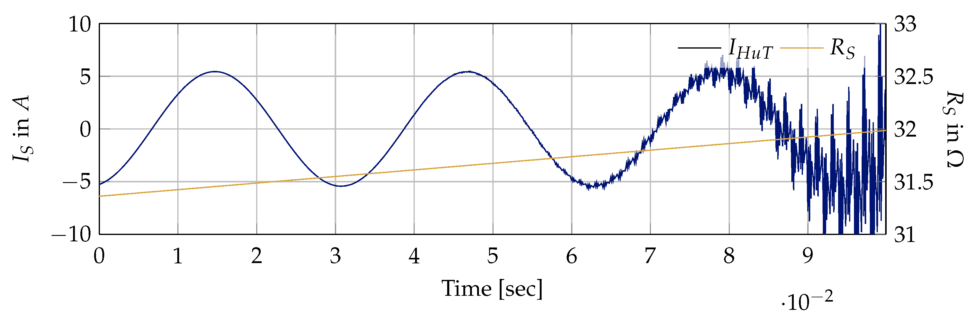
4.2. Experimental PHiL Stability Analysis

The analytic and simulative stability analysis from Section 3 is validated in the Microgrid, Energy Storage and Power Hardware-in-the-Loop Laboratory in collaboration with the Real-Time Laboratory of the LEES. An experimental setup, according to Figure 7, will be analyzed in this section with different PIs: a switching inverter and a linear inverter. The limits of stable operation are measured and will be compared against the simulative and the theoretical approach.

The virtual part of the PHiL circuit is implemented in RSCAD (RSCAD Software Version 5.014.1, RTDS Technologies Inc., Winnipeg, Canada) (see Figure 15) for RTS on a RTDS NovaCor™ real time simulator.

Both the switching and the linear amplifier are interfaced with the RTS with optical fiber AURORA communication. The HuT is a single phase resistive load with $1.85$ kW active power at $cos\phi =1$. The resistance is therefore $R_{HuT}=28.6 \Omega$.

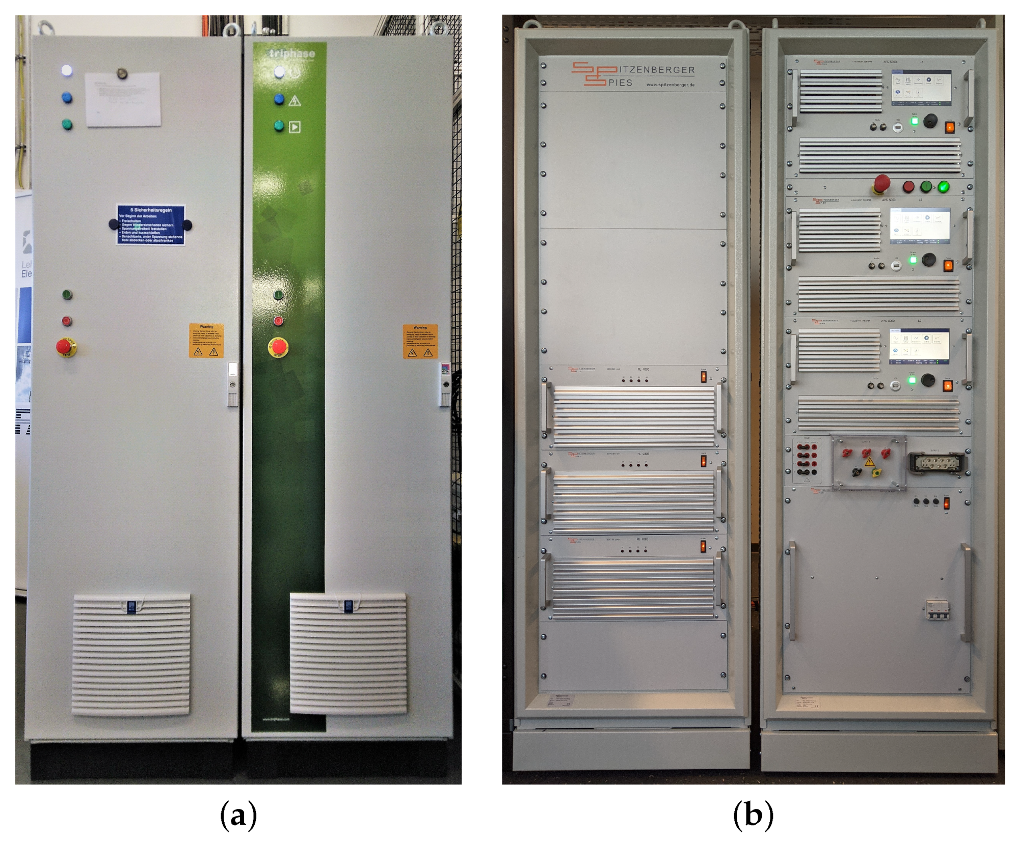
4.2.1. Experimental Setup with Switching Amplifier

The switching PI is a 4QA from the manufacturer Triphase NV, Holsbeek, Belgium with configuration: PM90I30PM12F120 with a rated power of $45$ kVA at the HuT-side and active grid feedback capability (see Figure 16a). The loop delay, that consists of RTS, communication and the delays within the 4QA was measured to an average of $590 \mathsf{\mu }$s.

4.2.2. Experimental Setup with Linear Amplifier

For comparison, the setup with the linear inverter is identical, regarding the HuT and RTS model. The linear amplifier is a 4QA of the manufacturer Spitzenberger & Spies, Viechtach, Germany of type DM 15000/APS/PHIL (see Figure 16b). The three-phase system consists of three synchronized single-phase APS 5000 amplifier modules as well as a resistor load bank as power sink. The loop time delay of the linear amplifier has been measured to approximately $125 \mathsf{\mu }$s, which includes communication and RTS. The same resistive load with $R_{HuT} = 28.6 \Omega$ is connected as HuT.

4.3. Comparison

The findings of the theoretical stability analysis of Section 3 are applied to the PHiL offline simulations and compared with the results of the practical validation in the following.

4.3.1. Ideal Power Interface

As a first approach, the influence of the power interface (PI) is neglected. An ideal PI with a unity gain of one is assumed. In addition, no FSF is applied. Thus, direct coupling of the RTS and the HuT side with time delay $T_d$ is achieved.

All experiments—simulative and real—in this section will be carried out with a resistive load $R_{HuT}=28.6 \Omega$. During simulation in MATLAB Simulink™ the variable resistance $R_S$ is increased until instability of the PHiL simulation occurs. As indicated in [6,18] instability in PHiL simulations appears as distortion and oscillation in the voltage and current waveform. To determine the critical impedance ratio the resistance $R_{S,lim}$ is determined when the PHiL simulation becomes unstable.

According to the NSC instability occurs when the impedance ratio exceeds one: $\frac{R_S}{R_{HuT}}>1$.

Thus, the system gets unstable if the resistance within the virtual part exceeds $R_{S,lim} = 28.6 \Omega$. However, within the offline emt-simulation in MATLAB Simulink™, as it can be obtained from Figure 17, only at $31.7 \Omega$ the sine waves signals of voltage and currents are starting to get distorted which indicates instability.

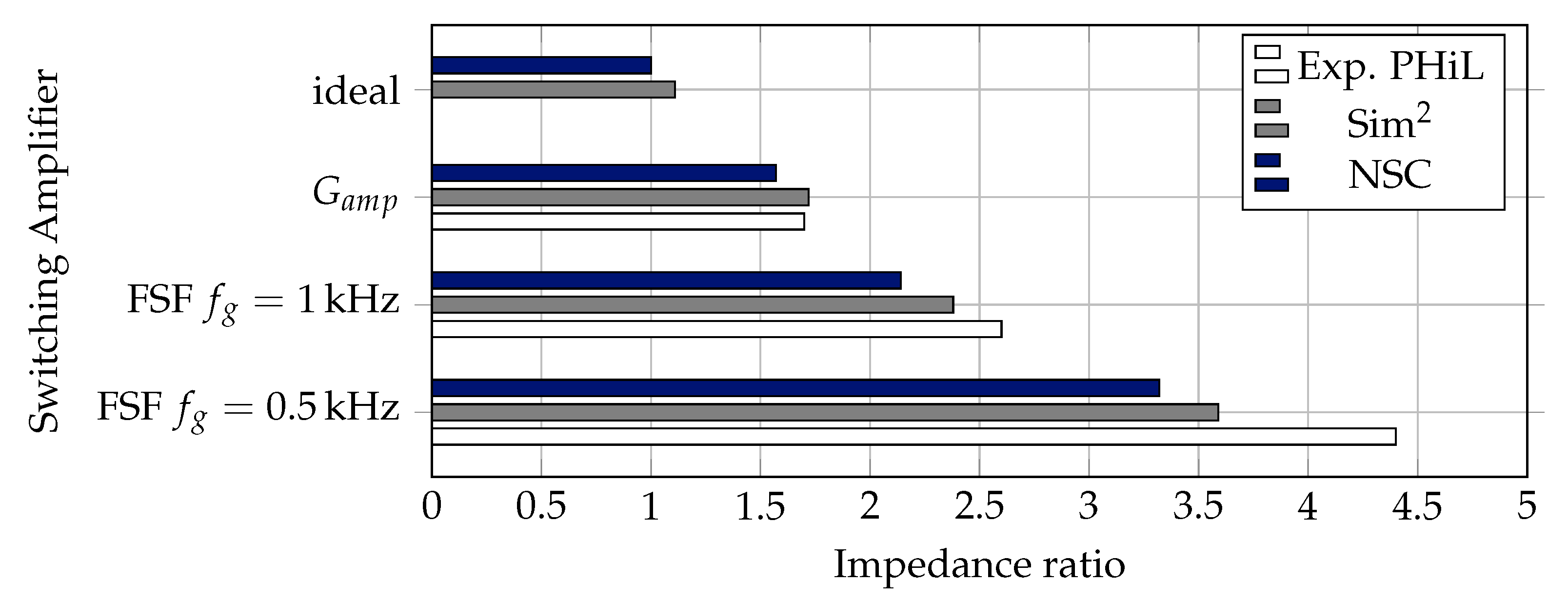
4.3.2. Influence of Amplifier Characteristics

As depicted in Section 3.2.5, the switching amplifier can be represented by a second-order transfer function and a time delay [32]. To characterize the switching amplifier, the step response has been measured, which is shown in Figure 18. A step function $V_{RTS}$ (0–230 V) has been applied within the RTS and is provided at the HuT by the 4QA. The measured voltage at the amplifier terminals $V_{HuT}$ is fed back to the RTS. Both signals (the step function and the measured voltage) have been recorded within the RTS with a sample rate of $62.5 \mathsf{\mu }$s.

To estimate the characteristics of the amplifier, the step response was approximated with the transfer function of a second order low-pass including a time delay:

$$\begin{array}{c}\hfill G_{approx.}\left(s\right)=G_{amp}\left(s\right)+G_{T_d}\left(s\right)=\frac{1}{2.2\times {10}^{-7}{s}^2+6.5\times {10}^{-4}s+1}{e}^{-s\times 590 \mathsf{\mu }s}\end{array}$$

(7)

The time delay of $590\mathsf{\mu }$s equals the total round trip delay $T_d$ of the PHiL simulation. The value has been confirmed by further measurements.

One part of the time delay is caused by the control of the converter and measurement delays, whereas another part by the communication and the discrete nature of the RTS. However, since the individual time delays cannot be measured exactly, in this case, the amplifier transfer function $G_{amp}\left(s\right)$ and the total time delay $G_{T_d}\left(s\right)$ are considered separately in the following.

By application of the amplifier transfer function $G_{amp}\left(s\right)$ the band limiting effect of the low-pass characteristics leads to an improvement in PHiL stability. According to NSC, the PHiL circuit can be determined unstable at a resistance ratio of $\frac{R_{RTS}}{R_{HuT}}>1.57$ ($R_{S,lim}=44.97 \Omega$), which is significantly higher than without consideration of $G_{amp}\left(s\right)$.

The offline emt-simulation in MATLAB Simulink™ indicated instability as $\frac{R_{RTS}}{R_{HuT}}>1.72$. The experimental PHiL simulation provides a smooth transition between stable and critically stable operation. Therefore $R_{S,lim}$, is rather a region than a discrete value. With the switching amplifier this is the case at around 47–50 $\Omega$ which results in an impedance ration of $\approx 1.7$. Only at $R_S>80\Omega$ the PHiL simulation is oscillating as strong as that the PI turns in error mode due to overcurrent limitation.

For comparison the step response of the linear amplifier is shown in Figure 19. Note the finer time resolution in comparison to Figure 18. According to the figure, the transfer function can be reduced to a time delay of two simulation time steps $2T_s$.

For noise reduction and anti aliasing the linear amplifier is equipped with a LPF. The filter is a first-order Butterworth low-pass with cut-off frequency $f_g=1.0$ MHz.

Applying Nyquist criterion this would lead to a theoretical ratio of $1.0138$. Which is only slightly above ideal interfacing due to the large value of $f_g$. It should be noted that without additional FSF no stable PHiL simulation could be achieved. A certain noise in the feedback current signal leads to an oscillation during the experiment.

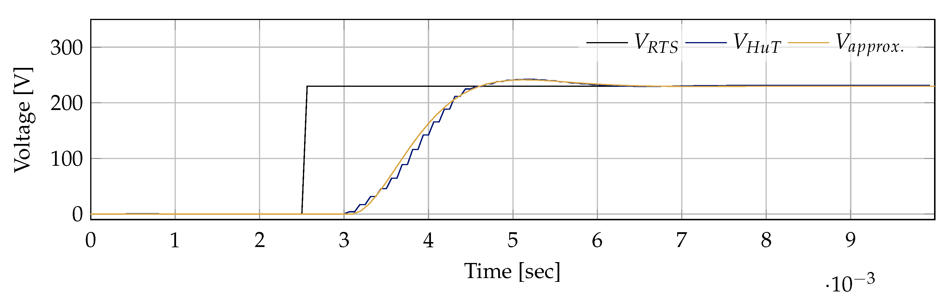
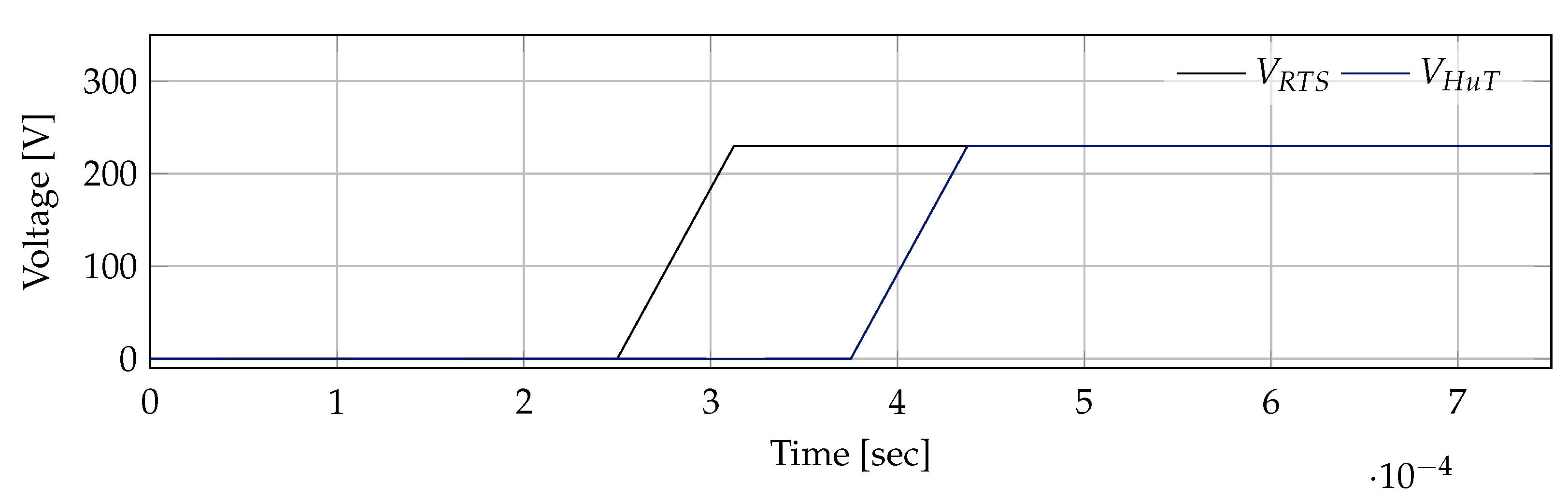
4.3.3. Influence of Feedback Signal Filtering and Time Delay

Further stability improvement can be obtained by the application of a LPF to the current feedback signal, as explained in Section 3.2. With a first-order LPF with $f_g=1.0$ kHz stability of the circuit with the switching amplifier can be obtained, according to NSC, up to $R_{S,lim}=61.2 \Omega$. Whereas, $R_{S,lim}=94.9 \Omega$ with filter cut-off frequency $f_g=0.5$ kHz. This is confirmed by the offline emt-simulation in MATLAB Simulink™ which indicated instability as $R_{S,lim}>68.1 \Omega$ at $f_g=1.0$ kHz and $R_{S,lim}>102.8 \Omega$ at $f_g=0.5$ kHz, resp. A graphical comparison of the results is shown in Figure 20.

Detailed data can be extracted from the Appendix A.

To validate the findings the respective LPF is implemented in the laboratory experiment into the current feedback path within RSCAD.

With filter cut-off frequency $f_g=1.0$ kHz and $f_g=0.5$ kHz the current through the HuT gets distorted at an impedance ratio of approximately $2.6$ (≈73–77 $\Omega$), and $4.4$ (≈122–127 $\Omega$), respectively.

With the linear inverter substantial extension of stable operation area can be realized by FSF. A LPF with cut off-frequency of $f_g=1.0$ kHz increases the critical impedance ratio to $13.13$ according to NSC. The simulated ratio provides a comparable value of $14.18$ whereas the experimental PHiL indicates instability at a ratio greater than $9.08$. A graphical comparison of the results with the linear amplifier is shown in Figure 21.

Detailed data can be extracted from the Appendix A.

For investigation of the influence of the loop delay on the power factor, an additional time lag is implemented into the current feedback signal path of the setup with the switchin amplifier. As already explained in Section 3.2.3, a time delay leads to a deviation in the power factor within the RTS.

At minimal loop delay ($T_d=590 \mathsf{\mu }$s), a power factor of $cos\phi =0.986$ occurs within the RTS in spite of purely resistive $R_S$ and $R_{HuT}$. In comparison, a power factor of $cos\phi =0.983$ can be calculated with Equation (5). Figure 22 compares calculated values of cosphi at several loop time delays with the measured values in the experimental PHiL.

During the experiment, it could be demonstrated that even in case of phase shift of ${180}^{\circ }$ stability is maintained whereas the power factor approaches $cos\phi =-1$.

5. PHiL for Grid Applications

A PHiL simulation enables the investigation of real physical equipment within simulated electrical power systems as a very flexible and realistic environment.

In the previous sections of this paper, it has been demonstrated, that stability of a PHiL simulation has to be studied carefully based on the ratio of $\frac{Z_S}{Z_{HuT}}$, the loop delay and limitations of bandwidth.

In [10] an impedance analyzer is described for a PV inverter which measures the response of an inverter at a change in grid voltage. In most PHiL simulation applications, however, the impedance of the HuT is not known exactly and, furthermore, it is changing during the simulation. In addition, the HuT can have nonlinear characteristics, which is the case with power electronic devices.

Thus, in the following, an application of a PHiL simulation will be presented to demonstrate the mitigation of stability issues in practice.

The behavior of a three-phase four-wire low-voltage distribution feeder, similar to the one in Figure 7a, which consist of a residential load and a PV system, shall be investigated. For this reason, the utility grid is replaced by a real-time model for simulation with voltage type ITM PHiL.

All parameters are listed in

Table 1. Parameter of the PHiL application example.

Grid voltage (50 Hz)	${\mathit{V}}_{\mathit{S}}$	$0.4$	kV
Grid impedance	$Z_{grid}$	$100+\mathrm{j}6.3$	m$\Omega$
Load impedance	$Z_L$	$28.6+\mathrm{j}0$	$\Omega$
LPF cut-off frequency	$f_{g,FSF}$	$1.0$	kHz
PV system rated power (three phase)	$P_{PV,n}$	$7.0$	kW

. According to the previous sections the impedance ratio of $Z_{RTS}$ to $Z_{HuT}$ is crucial regarding stability. However, $Z_{HuT}$, which is the total impedance of the PV system in this case, cannot be determined exactly. Furthermore $Z_{HuT}$ is nonlinear and changing during the experiment.

To ensure a stable operation during the whole experiment stability improvements through FSF are implemented.

The household peak load (three-phase) in this example is assumed to be $5.6$ kW at $cos\phi \approx 1$. Thus, the minimal impedance per phase equals $Z_{HuT,min}=28.6+\mathrm{j}0\Omega$. The rooftop PV system consists of a system with a conventional inverter with a rated power of $7$ kWp. At the begin of the experiment the PV system is still switched off. Due to the resistive-inductive grid the PHiL simulation would be unstable according to Section 3.2.2 due to $L_{HuT}=0$ and therefore $L_S>L_{HuT}$. However, with the transfer function of the switching inverter $G_{amp}$ the circuit can be stabilized which can be validated during the experiment.

After the begin of the experiment the PV system is switched on and starts to synchronize with the grid. Although detailed characteristics of the PV inverter are not known, current oscillations can be observed at the moment of synchronization which leads to instability.

To guarantee a stable PHiL simulation, FSF is applied. The application of a first order LPF with cut-off frequency of $f_g=1$ kHz grantees a stable PHiL simulation. Over the whole operating range of the load and up to $4$ kW PV active power (restricted by irradiation during the test) no stability issues were observed.

Although stability is improved through FSF, simulation accuracy diminishes. According to Section 3.2.3 the additional phase shift induced by the LPF influences the power-factor in the RTS. In this exemplary PHiL simulation $T_d=590 \mathsf{\mu }$s and the phase shift due to the LPF at the fundamental frequency ($f_s=50$ Hz) corresponds to $966 \mathsf{\mu }$s. Thus, the total shift between voltage in the RTS and the feedback current adds up to 1.56 ms. According to Equation (5) the power factor of the resistive load is reduced to $cos\phi =0.88$, which can be confirmed by the experimental PHiL simulation (see Figure 22). A possible mitigation is the introduction of an additional time delay of $T_{comp}$ = 0.01844 s. In Figure 23 the additional time delay $T_{comp}$ is applied at a simulation time of two seconds. Thus, the phase between the simulated voltage $V_{RTS}$ and the feedback current $I_S$ is reduced to zero. Power factor correction through an additional time delay, however, reduces the accuracy of transient events. Therefore [10] presents a filter with a compensator to mitigate phase delay. Another mitigation would be the application of a linear inverter for PI. Due to reduced loop delay with a linear amplifier, stability is guaranteed even if a LPF with higher cut-off frequency is applied, which in turn minimizes power factor deviations.

6. Discussion

The comparison of the experimental stability limits match the simulative and theoretical approach. The theoretical limits of $R_{s,lim}$ estimated with NSC are systematically lower than the values from the simulation in MATLAB Simulink™ due to the fact, that NSC analyzes the whole frequency spectrum whereas the emt-simulation is restricted to $f_s=50$ Hz. NSC therefore provides a rather pessimistic estimation. Furthermore the values of $R_{s,lim}$ from the laboratory experiment with the switching amplifier exceed the theoretical and simulative results in most cases. This can be explained due to stabilizing features which are included in the inverter control, e.g., harmonics compensation. Accordingly, the resulting impedance ratio with the linear amplifier is lower than anticipated because there is no additional stabilizing control. On the contrary disturbances occur in the laboratory experiment which are not present in simulation.

A comparison of the results with both linear and switching amplifier clearly demonstrates the advantage of reduced time delays and faster simulation time steps.

In the context of this work, estimation of the amplifier transfer function with the step response shows to be sufficient. However, further analysis could be done to improve the knowledge on amplifier characteristics, e.g., frequency behavior and analysis with increased resolution.

The analysis and explanations within this work have been restricted to the voltage type ITM but can easily be extended to current type ITM and other IAs. In [15] both voltage and current type ITM are presented.

Stability improvement with FSF has been demonstrated at the example of a first order low-pass filter as an effective way of improving PHiL stability. However, at the expense of simulation accuracy, as Section 4 could demonstrate, with good accordance between theoretical approach and experimental results. Improved low-pass filter types can reduce the power factor deviation. Ref. [10] presents a filter with a compensator to mitigate phase delay.

The experimental verification of the findings from Section 3 has been restricted to a resistive load in Section 4, given the limited frame of this paper, but will be extended to complex impedances in future studies as well as an additional investigation of a nonlinear HuT.

7. Conclusions

In this paper, a general analysis of PHiL stability based on Nyquist stability criterion applied to the transfer function of a simplified circuit has been shown. To the major influence factors: impedance ratio, time delay, amplifier characteristics and low-pass filtering, special consideration is given. The findings have been applied to an offline model of an exemplary PHiL simulation case, which was implemented in MATLAB Simulink™, to investigate the margin of stable PHiL simulation. The modeling approach was validated with an experimental PHiL setup using a linear and a switching amplifier as power interface in comparison. Apart from a good correlation between theory, simulation and laboratory experiment, the results demonstrate that even inherently unstable PHiL cases can be stabilized with feedback signal filtering method with both, linear and switching inverters. However, due to substantial lower loop delays, linear inverters require less intensive stabilization which has a positive effect on simulation accuracy.

References

1. Bruckner, T.; Bashmakov, I.A.; Mulugetta, Y.; Chum, H.; de la Vega Navarro, A.; Edmonds, J.; Faaij, A.; Fungtammasan, B.; Garg, A.; Hertwich, E.; et al. Energy Systems. In Climate Change 2014: Mitigation of Climate Change. Contribution of Working Group III to the Fifth Assessment Report of the Intergovernmental Panel on Climate Change (IPCC); Cambridge University Press: Cambridge, UK; New York, NY, USA, 2014. [Google Scholar]
2. ISGAN Annex 6 Power T& D Systems—Ancillary Services from Distributed Energy Sources for a Secure and Affordable European System: Main Results from the SmartNet Projects. 2019. Available online: https://www.iea-isgan.org/smartnet (accessed on 20 December 2021).
3. Lauss, G.; Strunz, K. Accurate and Stable Hardware-in-the-Loop (HIL) Real-Time Simulation of Integrated Power Electronics and Power Systems. IEEE Trans. Power Electron. 2021, 9, 10920–10932. [Google Scholar] [CrossRef]
4. Guillo-Sansano, E.S.; Mazheruddin, H.; Roscoe, A.J.; Burt, G.M.; Coffele, F. Characterization of Time Delay in Power Hardware in the Loop Setups. IEEE Trans. Ind. Electron. 2021, 3, 2703–2713. [Google Scholar] [CrossRef]
5. Nzimako, O.; Wierckx, R. Stability and Accuracy Evaluation of a Power Hardware in the Loop (PHIL) Interface with a Photovoltaic Micro-Inverter; IECON: Yokohama, Japan, 2015. [Google Scholar]
6. Wang, S.; Li, B.; Xu, Z.; Zhao, X.; Xu, D. A Precise Stability Criterion for Power Hardware-in-the-Loop Simulation System. In Proceedings of the 10th International Conference on Power Electronics and ECCE Asia, Busan, Korea, 27–30 May 2019. [Google Scholar]
7. Dolenc, J.; Bozicek, A.; Blazic, B. Stability Analysis of an Ideal-Transformer-Model Interface Algorithm. In Proceedings of the 7th International Youth Conference on Energy, Bled, Slovenia, 3–6 July 2019. [Google Scholar] [CrossRef]
8. Riccobono, A.; Helmedag, A.; Berthold, A.; Averous, N.R.; de Doncker, R.W.; Monti, A. Stability and Accuracy Considerations of Power Hardware- in-the-Loop Test Benches for Wind Turbines. IFAC-PapersOnLine 2017, 1, 10977–10984. [Google Scholar] [CrossRef]
9. Li, F.; Huang, Y.; Wu, F.; Zhang, X.; Zhao, W. Power-Hardware-in-the-Loop Stability Analysis of Inverter. In Proceedings of the 22nd International Conference on Electrical Machines and Systems (ICEMS), Habin, China, 11–14 August 2019. [Google Scholar] [CrossRef]
10. Pokharel, M.; Ho, C.N.M. Stability Analysis of Power Hardware-in-the-Loop Architecture With Solar Inverter. IEEE Trans. Ind. Electron. 2021, 5, 4309–4319. [Google Scholar] [CrossRef]
11. Marks, N.D.; Kong, W.Y.; Birt, D.S. Stability of a Switched Mode Power Amplifier Interface for Power Hardware-in-the-Loop. IEEE Trans. Ind. Electron. 2018, 11, 8445–8454. [Google Scholar] [CrossRef]
12. Markou, A.; Kleftakis, V.; Kotsampopoulos, P.; Hatziargyriou, N. Improving Existing Methods for Stable and More Accurate Power Hardware-in-the-Loop Experiments; IEEE International Symposium on Industrial Electronics, Institute of Electrical and Electronics Engineers (ISIE): Edinburgh, UK, 2017. [Google Scholar] [CrossRef]
13. Barakos, D.; Kotsampopoulos, P.; Vassilakis, A.; Kleftakis, V.; Hatziargyriou, N. Methods for Stability and Accuracy Evaluation of Power Hardware in the Loop Simulations. In Proceedings of the Mediterranean Conference on Power Generation, Transmission Distribution and Energy Convers(MedPower), Athens, Greece, 2–5 November 2014. [Google Scholar] [CrossRef]
14. Lauss, G.; Lehfuß, F.; Viehweider, A.; Strasser, T. Power Hardware in the Loop Simulation with Feedback Current Filtering for Electric Systems. In Proceedings of the 37th Annual Conference of the IEEE Industrial Electronics Society (IECON 2011), Melbourne, Australia, 7–10 November 2011. [Google Scholar] [CrossRef]
15. Ren, W.; Steurer, M.; Baldwin, T.L. Improve the Stability and the Accuracy of Power Hardware-in-the-Loop Simulation by Selecting Appropriate Interface Algorithms. IEEE Trans. Ind. Appl. 2008, 4, 1286–1294. [Google Scholar] [CrossRef]
16. Lamo, P.; de Castro, A.; Sanchez, A.; Ruiz, G.A.; Azcondo, F.J.; Pigazo, A. Hardware-in-the-Loop and Digital Control Techniques Applied to Single-Phase PFC Converters. Electronics 2021, 10, 1563. [Google Scholar] [CrossRef]
17. Ihrens, J.; Möws, S.; Wilkening, L.; Kern, T.A.; Becker, C. The Impact of Time Delays for Power Hardware-in-the-Loop Investigations. Energies 2021, 14, 3154. [Google Scholar] [CrossRef]
18. Brandl, R. Operational Range of Several Interface Algorithms for Different Power Hardware-in-the-Loop Setups. Energies 2017, 10, 1946. [Google Scholar] [CrossRef] [Green Version]
19. Kotsampopoulos, P.; Lagos, D.; Hatziargyriou, N.; Faruque, M.O.; Lauss, G.; Nzimako, O.; Forsyth, P.; Steurer, M.; Ponci, F.; Monti, A.; et al. A Benchmark System for Hardware-in-the-Loop Testing of Distributed Energy Resources. IEEE Power Energy Technol. Syst. J. 2018, 3, 94–103. [Google Scholar] [CrossRef]
20. García-Martínez, E.; Sanz, J.F.; Muñoz-Cruzado, J.; Perié, J.M. A Review of PHIL Testing for Smart Grids—Selection Guide, Classification and Online Database Analysis. Electronics 2020, 9, 382. [Google Scholar] [CrossRef] [Green Version]
21. Edrington, C.S.; Steurer, M.; Langston, J.; El-Mezyani, T.; Schoder, K. Role of Power Hardware in the Loop in Modeling and Simulation for Experimentation in Power and Energy Systems. Proc. IEEE 2015, 12, 2401–2409. [Google Scholar] [CrossRef]
22. Faruque, M.O.; Strasser, T.; Lauss, G.; Jalili-Marandi, V.; Forsyth, P.; Dufour, C.; Dinavahi, V.; Monti, A.; Kotsampopoulos, P.; Martinez, J.A.; et al. Real-Time Simulation Technologies for Power Systems Design, Testing, and Analysis. IEEE Power Energy Technol. Syst. J. 2015, 10, 63–73. [Google Scholar] [CrossRef]
23. Dargahi, M.; Ghosh, A.; Ledwich, G.; Zare, F. Studies in power hardware in the loop (PHIL) simulation using real-time digital simulator (RTDS). In Proceedings of the IEEE International Conference on Power Electronics, Drives and Energy Systems (PEDES), Bengaluru, India, 16–19 December 2012. [Google Scholar]
24. Lehfuss, F.; Lauss, G.; Kotsampopoulos, P.; Hatziargyriou, N.; Crolla, P.; Roscoe, A. Comparison of multiple power amplification types for power Hardware-in-the-Loop applications. In IEEE Complexity in Engineering (COMPENG); IEEE: Piscataway, NJ, USA, 2012; pp. 1–6. [Google Scholar]
25. Muhammad, M.; Behrends, H.; Geißendörfer, S.; Maydell, K.V.; Agert, C. Power Hardware-in-the-Loop: Response of Power Components in Real-Time Grid Simulation Environment. Energies 2021, 14, 593. [Google Scholar] [CrossRef]
26. Noureen, S.S.; Shamim, N.; Roy, V.; Bayne, S.B. Real-Time Digital Simulators: A Comprehensive Study on System Overview, Application, and Importance. Int. J. Res. Eng. 2017, 266–277. [Google Scholar] [CrossRef]
27. Kuffel, R.; Forsyth, P.; Peters, C. The Role and Importance of Real Time Digital Simulation in the Development and Testing of Power System Control and Protection Equipment. IFAC-PapersOnLine 2016, 27, 178–182. [Google Scholar] [CrossRef]
28. CIGRE Working Group B4.57, Guide for the Development of Models for HVDC Converters in a HVDC Grid. 2017. Available online: https://e-cigre.org/publication/604 (accessed on 20 December 2021).
29. Nzale, W.; Mahseredjian, J.; Kocar, I.; Fu, X.; Dufour, C. Two Variable Time-Step Algorithms for Simulation of Transients. In Proceedings of the 2019 IEEE Milan PowerTech, Milan, Italy, 23–27 June 2019; pp. 1–6. [Google Scholar]
30. Resch, S.; Och, S.; Luther, M. Conception, Modelling Approach and Practical Implementation of a Hybrid Laboratory-Based Microgrid. In Proceedings of the Conference on Sustainable Energy Supply and Energy Storage Systems, Hamburg, Germany, 20–21 September 2018. [Google Scholar]
31. Resch, S.; Luther, M. Reduction of Battery-Aging of a Hybrid Lithium-Ion and Vanadium-Redox-Flow Storage System in a Microgrid Application. In Proceedings of the 2nd IEEE International Conference on Industrial Electronics for Sustainable Energy Systems (IESES), Cagliari, Italy, 1–3 September 2020; pp. 80–85. [Google Scholar]
32. Ren, W. Accuracy Evaluation of Power Hardware-in-the-Loop (PHIL) Simulation. Ph.D. Thesis, Florida State University, Tallahassee, FL, USA, 2007. [Google Scholar]
33. Haineault, M.; Gregoire, L.A.; Paquin, J.N.; Bélanger, J. Key Considerations When Selecting Amplifiers for your Power Hardware-in-the-Loop (PHIL) Testbed; OPAL-RT TECHNOLOGIES Inc.: Montréal, QC, Canada, 2019. [Google Scholar]
34. García-Martínez, E.; Ballestín, J.; Muñoz-Cruzado, J.; Sanz, J.F. Analysis of a switched and linear power amplifier for Power Hardware-in-the-Loop testing of Smartgrid systems. In Proceedings of the 24th IEEE International Conference on Emerging Technologies and Factory Automation (ETFA), Zaragoza, Spain, 1–10 September 2019. [Google Scholar]
35. Dmitriev-Zdorov, V.B. Generalized coupling as a way to improve the convergence in relaxation-based solvers. In Proceedings of the EURO-DAC EUROVHDL, Geneva, Switzerland, 16–20 September 1996; pp. 15–20. [Google Scholar]
36. Hui, S.Y.R.; Fung, K.K.; Christopoulos, C. Decoupled simulation of DC-linked power electronic systems using transmission-line links. IEEE Trans. Power Electron. 1994, 9, 85–91. [Google Scholar] [CrossRef]
37. Dargahi, M.; Ghosh, A.; Ledwich, G. Stability Synthesis of Power Hardware-in-the-Loop (PHIL) Simulation. In Proceedings of the IEEE PES General Meeting, National Harbor, MD, USA, 27–31 July 2014; pp. 1–5. [Google Scholar] [CrossRef] [Green Version]
38. Westphal, L.C. Handbook of Control Systems Engineering, 2nd ed.; Springer: Boston, MA, USA, 2018. [Google Scholar] [CrossRef]
39. Tremblay, O.; Fortin–Blanchette, H.; Gagnon, R.; Brissette, Y. Contribution to stability analysis of power hardware–in–the–loop simulators. IET Gener. Transm. Distrib. 2017, 12, 3073–3079. [Google Scholar] [CrossRef]
Figure 1. Setup of the Microgrid, Energy Storage and Power Hardware-in-the-Loop Laboratory in collaboration with the Real Time Laboratory of the LEES.
Electronics 11 00007 g001
Figure 2. Major accuracy deviations that are introduced in a system through PHiL simulation.
Electronics 11 00007 g002
Figure 3. Voltage-type ITM interfacing algorithm for PHiL simulation.
Electronics 11 00007 g003
Figure 4. PCD interfacing algorithm for PHiL simulation.
Electronics 11 00007 g004
Figure 5. DIM interfacing algorithm for PHiL simulation.
Electronics 11 00007 g005
Figure 6. Voltage-type ITM with FSF.
Electronics 11 00007 g006
Figure 7. Exemplary low-voltage grid reduced to a minimal PHiL circuit with voltage-type ITM IA (a) Exemplary low-voltage grid; (b) Simplified equivalent circuit of the low-voltage grid; (c) Equivalent circuit with voltage-type ITM IA.
Electronics 11 00007 g007
Figure 8. Block diagram of a voltage type ITM PHiL.
Electronics 11 00007 g008
Figure 9. Nyquist curve for resistive impedance PHiL in dependence of the quotient of resistance R S over R H u T .
Electronics 11 00007 g009
Figure 10. Locus plot with the angular frequency as an additional dimension.
Electronics 11 00007 g010
Figure 11. Locus plot of FSF-ITM with different cut-off frequencies with the angular frequency as an additional dimension.
Electronics 11 00007 g011
Figure 12. Locus plot of ITM PHiL in dependence of the loop time delay with the angular frequency as an additional dimension.
Electronics 11 00007 g012
Figure 13. Locus plot of voltage type ITM PHiL with different loop time delays and low pass cut of frequencies.
Electronics 11 00007 g013
Figure 14. MATLAB Simulink™ model for validation of the stability analysis.
Electronics 11 00007 g014
Figure 15. Virtual part of the PHiL simulation modeled in RSCAD.
Electronics 11 00007 g015
Figure 16. Four quadrant amplifiers applied in the experimental PHiL setup. (a) Switching amplifier; (b) Linear amplifier.
Electronics 11 00007 g016
Figure 17. Feedback current with rising R S until stability limit is reached.
Electronics 11 00007 g017
Figure 18. Step response of the switching inverter in comparison to the approximation.
Electronics 11 00007 g018
Figure 19. Step response of the linear amplifier.
Electronics 11 00007 g019
Figure 20. Impedance ratio as stability limit for analysis with a switching inverter.
Electronics 11 00007 g020
Figure 21. Impedance ratio as stability limit for analysis with a linear inverter.
Electronics 11 00007 g021
Figure 22. Relation between loop delay and cosphi in comparison between theory and practical PHiL simulation.
Electronics 11 00007 g022
Figure 23. Power factor correction with an additional time delay.
Electronics 11 00007 g023