1. Introduction
Traditionally, robots have been aiding humans in many areas as they are more capable and often better equipped to deal with tasks that include high repeatability. The advancements in the areas of batteries, sensors, artificial intelligence (AI), and machine learning (ML) open new horizons and application domains as they allow robots and, more precisely, mobile robots to perform more complex tasks [
1]. These can be anything from driving and delivering packages to cleaning jobs [
2]. There are many mobile robots designed for indoor-cleaning operation, however there are less low-cost robots designed for outdoor-cleaning operations with the ability to remove medium-size objects [
3]. This is very important when the cleaning must be done under difficult environmental conditions, such as heat or cold or when cleaning materials that are hazardous for humans or the environment [
4]. In the current study, trash widespread at picnic spots, on or near pavements, washed by waves onto sandy or pebbly beaches and other such outdoor locations were focused upon. Keeping a pragmatic outlook in mind, this robot was designed to conquer the regular challenges of outdoor land terrains and obstacles. A completely autonomous robot was capable of performing activities like trash detection, obstacle avoidance, robotic path-planning, and robotic motion control automatically.
A unique flap-bucket system was used in the mechanical design, which enabled trash collection through a sweep where multiple trash objects of varying sizes were collected simultaneously, unlike when a robotic hand is used, which can only pick up a single item at a time. The novel approach of assimilating the six-wheeled Rocker-Bogie mechanism into the robot for its smooth movement on multiple outdoor terrains made it perfect for outdoor trash collection.
The use of modern technologies of artificial intelligence in this robot facilitated making it smart and autonomous. Image processing and deep learning constituted the computer vision model. A more advanced method, namely transfer learning, was used in the object detection model building. Varied models and the latest versions of these models at the time like MaskRCNN, YOLOv4, and YOLOv4-tiny were experimented on and analyzed comprehensively. Experimental results demonstrated that YOLOv4-tiny performed the fastest detection, thereby making it apt for usage for detection in real-time.
Path-planning algorithm made the robot truly autonomous, as once the coordinates of the area to be cleaned were fed to the robot, it did not require any further assistance. It autonomously searched for the trash, avoided obstacles, and generated its own path accordingly. The sensors provided all the necessary information required for the feedback mechanisms of the robot and helped in its decision-making process.
The rest of the paper is organized as follows.
Section 2 discusses the previous works and compares them with our current robot.
Section 3 contains a backdrop of the materials and methods used to build this robot.
Section 4 elaborates on the structure of the robot and the functioning of each mechanical and electronic part.
Section 5 provides insights and a step-by-step procedure for building the object-detection model to detect trash. In
Section 6, the software implementation into the Raspberry Pi and the path planning followed by the autonomous robot are discussed in detail.
Section 7 evaluates the proposed design in solid works, using various generated terrains.
Section 8 portrays the results obtained from the experimental analysis and a comparative study. Finally,
Section 9 summarizes this work.
2. Related Work
This section discusses the existing work in the field of trash-cleaning robots. In the mechanical design of the robot built to operate on water bodies, a conveyor belt was used to collect floating trash from the surface of rivers [
5,
6,
7]. In [
8], the robot employed broom bristles to sweep trash controlled by a servo motor and the collector bin was opened periodically to empty this trash. Some of the trash-collecting robots used a robotic arm to carry out the process of trash-picking. The degree of freedom of the manipulator that was used varied from two degrees of freedom to seven degrees of freedom. The end-effector of the manipulator played the role of grasping the concerned object, which was trash [
9].
The remote-controlled robots were controlled through mobile applications via Bluetooth like in [
10,
11,
12], or via Wi-Fi like in [
8,
13,
14]. LIDAR (Light Detection and Ranging) and GPS (Global Positioning System) were incorporated in some of the trash-collecting robots and prototypes [
15,
16]. A modified YOLOv3 was proposed for garbage detection where the original three-scale detection was changed to two-scale to cope with speedy processing in real-time [
17]. A lightweight neural network for garbage detection based on AlexNet-SSD model was used in [
18] where the traditional VGG network was replaced by AlexNet for the base. In [
19], a lightweight SSD model was developed, where a focal loss function for smooth handling of class imbalance was used as well as a new feature pyramid for achieving strong semantics on all scales; here, the ResNet was used as the base network in place of the original VGG network.
The processing for path planning was carried out in a ROS (Robotic Operating System) where map segmentation was implemented. An exploration algorithm, namely A * algorithm, was used for navigation of the robot while avoiding any obstacles. In this algorithm, the path that had the minimum cost to the goal, while considering the Euclidean distance, was taken [
20].
Comparative Study
Some of the previous works were shortlisted and then their capabilities were compared with the OATCR robot in
Table 1. In [
12], the robot mostly worked autonomously while it also transmitted the visuals through the IP camera for effective oversight in some situations, in which case the app was used to control it while the shovel in front picked up the trash when rotated, and the sensors made obstacle avoidance possible for the robot. In [
21], the robot was truly autonomous as it could move around taking the optimal path while avoiding obstacles and detect the trash on its own; it relied on the Deep Learning, Extended Kalman Filter, and PID control to smoothly operate on its own, while a four-d.o.f. (Degree of Freedom) robotic arm was used to pick up the trash from the grass. In [
22], the robot was controlled remotely via radio signals, while dragging a mechanism which continuously ploughed and sieved the sand to remove the solid particles and store them in a bin. In [
20], a pre-existing Care-O-Bot platform was used for the robot to explore the area, detect dirt, clear trash cans, and vacuum as it contained the required features like a seven-d.o.f. Robotic arm which could change the tool based on the task that needed to be performed; it had a RGB-D sensor for detection and the computational power to perform tasks like navigation and image processing in real time. In [
23], Toyota’s HSR platform was used, which consists of a RGB-D camera, a four-d.o.f. arm, various built-in sensors as well as powerful computers. The robot was completely autonomous; it was able to generate the path, avoid obstacles, and map its surrounding area. Two CNN networks were used, FCN8 for the floor and wall segmentation and a SSD mobile network which detected any obstacles. In [
24], the robot used CNN for detecting the trash on a Raspberry Pi while the Arduino controlled the motors and a four-d.o.f. robotic arm was used to pick up the detected trash. In [
13], the robot had two modes, autonomous and manual. In the autonomous mode, the robot picked up any sufficiently small object and treated bigger objects as obstacles. While in the manual mode, the robot was controlled through a mobile app via Wi-Fi. The robot had a robotic arm through which it picked up the objects and separated them into metallic or non-metallic groups. In [
11], the robot could be controlled remotely through an app or autonomously, in which it avoided any obstacles until a yellow color was detected by its camera. After the detection, it moved towards the yellow color and opened its lid for a few seconds. There was a suction fan placed below the robot to work as a vacuum and suck up any dust. In [
9], the robot moved autonomously. It used a camera and computer vision to detect cans (trash) by comparing the frame with stored images and a two-d.o.f. robotic arm to pick up the trash. In [
25], the robot was used to collect floating trash from the water bodies. It consisted of a binocular camera, a three-d.o.f. robotic arm to pick the trash, and four propellers to move. The visuals from the binocular camera were sent to a PC for the image processing and the results were sent back to the robot. YOLOv3 was used for the detection of the trash and the sliding-mode controller was used (SMC) for steering the robot.
3. Materials and Methods
The graphical design and modelling of the mechanical structure was carried out in SolidWorks 2018. SolidWorks is a 3D modelling software that is used for generating 3D designs. It has integrated tools to provide analytical and design automation to simulate the real-world behavior such as kinematics, dynamics, stress, deflection, vibration, temperatures, or fluid flow. It was developed by Dassault Systèmes as a CAD (Computer Aided Design) and a CAE (Computer Aided Engineering) software.
The Raspberry Pi 4 Model B and Arduino UNO were the two microcontrollers used to carry out cognitive decisions for the robot. The Raspberry Pi 4 Model B was the latest at the time and was substantially more capable than its previous models. With the increase in clock speed to 1.5 GHz and RAM from 1 GB to 2 GB and with 4 GB variants available, the benchmark score is 4 to 5 times better in performance than that of its predecessor. Similar to the function of brain and spine in humans, the Raspberry Pi had the function of running the heavier computational tasks such as image processing and robot tracking, while the Arduino UNO performed intermediary tasks such as obstacle avoidance and path planning, which lifted some load from the Raspberry Pi.
Geared DC motors, Stepper motors, and Servo motors served different purposes. Geared DC motors played a role where the precision of moments was not the primary concern/objective/motive or where the system was a closed loop with a sensor working as a feedback loop, such as in the movement of the robot. The stepper motors were used to provide accuracy in control with high torque in an open-loop system. Disparate to the earlier-mentioned motors, the servo motors provided excellent control over its accuracy in movement while high torque was not a major requirement.
To control these motors, motor controllers were required. Motor controllers are very useful circuits which can be used to control the motor’s directions and speeds. The L298N motor driver consists of an H-bridge circuit which is able to switch the polarity of voltage in the output, changing the direction of the motor, whereas the PWM control allows for a change in speed according to the input value. It was used to control the Geared DC motors. Meanwhile, the TB6600 stepper motor driver is capable of controlling two-phase stepper motors. It has two enable pins, two direction pins, and two pulse pins to communicate with the microcontroller and control the stepper motors.
Ultrasonic sensors were used to detect any obstacle in the path and avoid them, as they are able to perform adequately even in an outdoor environment, as opposed to an IR sensor, which may not be able work properly due to the infrared radiation from the sun. The infrared sensor was used inside the trash-collector bin of the robot to detect when it was filled. As the IR sensor was positioned inside the robot, it was protected from the radiation of the sun and thereby was able to work efficiently/suitably. The Neo 6M GPS module was used to track the location of the robot at all times. The sensor contained a backup battery in case the power supply failed, which was an important feature to extract the robot from any system or tackle power failure. A webcam inputted visuals of its surroundings to the robot and worked as eyes for the robot, and a Triple-Axis Compass Magnetometer Sensor Module guided the robot in the right direction.
Raspbian was installed in the Raspberry Pi micro-processor, which was its operating system. Since it was Debian-based, the commands were similar to bash shell in Linux, where it was addressed as sudo each time a command was given. The Picamera library was installed and then imported in order to control the camera module via Raspberry Pi. Programming in Arduino IDE was performed in the C language. Object classification, along with object localization, was a task required to be executed by the Outdoor Autonomous Robot. Object classification provided information about whether the object to be detected was present or not, whereas object localization apprized the robot of the location of the detected object in the images captured by the camera in real-time. In this case, the concerned object was trash.
There were some essential libraries which were utilized in the programming for image-processing: Deep Learning and Computer Vision in Python. Keras was one such neural network library and Tensorflow provided a wide range of tools and libraries for machine learning. Numpy was a powerful tool to perform mathematical computations and Matplotlib was used for plotting bounding boxes and for predicting scores and labels on the input images. OpenCV was used for detection in real time.
In the model evaluation process, IoU and mAP contributed significantly. Intersection over Union (IoU) is an evaluation metric used to compute the accuracy of an object-detection model on a specific dataset. It is also known as the Jaccard Index, which is calculated as (1).
where J is the Jaccard distance, A is Set 1, and B is Set 2
IoU gives the deviation of predicted truth annotation from the output of the computer vision model and the actual ground truth annotation.
Furthermore,
where
TP stands for true positive and
FP stands for false positive, thereby the denominator being the positive examples in the test set.
where
FN stands for false negative, thereby the denominator being the actual number of examples in the test set therefore helping in evaluating the ability of the model to detect correctly.
where AP stands for Average Precision, mAP for mean Average Precision,
N for total number of objects in all categories [
26].
4. Robotic Structure
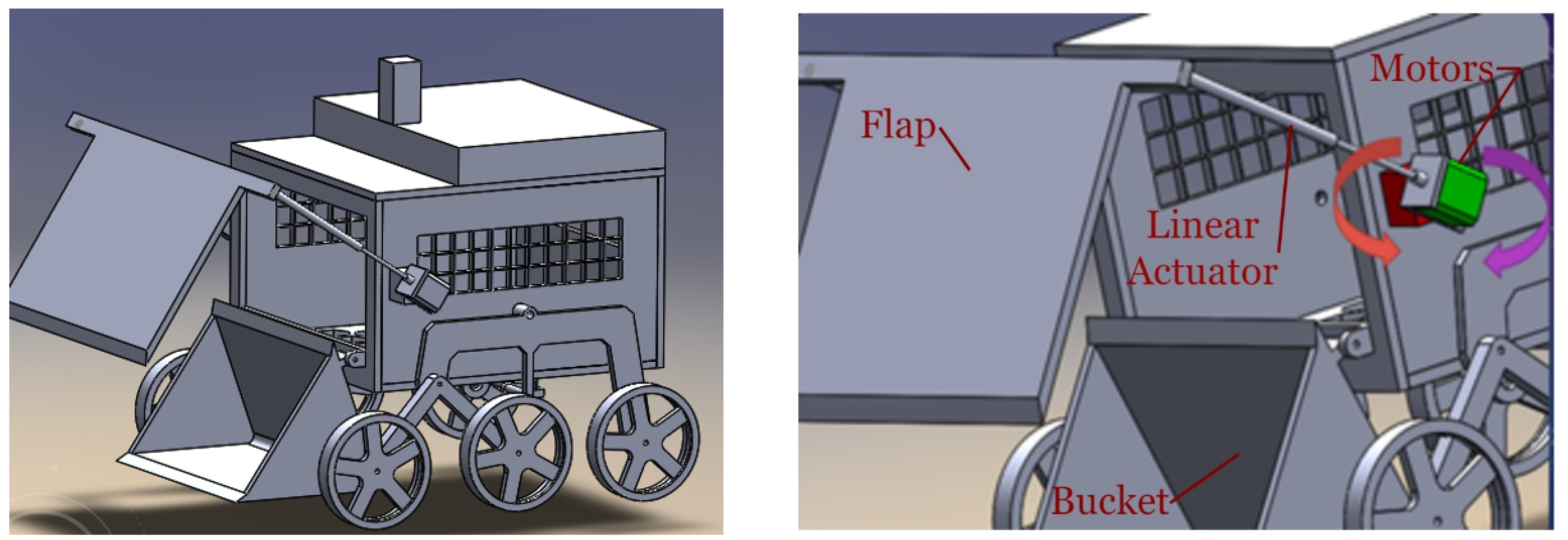
The robot had an overall cuboidal structure with a hollow interior which acted as a trash-collector bin. The rocker-bogie mechanism was adopted for suspension and afforded the robot more flexibility to move through different surfaces so that it could move over uneven surfaces without toppling; hence, six wheels needed to be used. It used six motors, one for each wheel, therefore being a six-wheel drive. A flap was attached to the anterior part of the robot. Movement of this flap was controlled by two linear actuators and two stepper motors. The linear actuators were mounted on a rotatable platform which was powered by the two stepper motors so as to enable the flap’s horizontal as well as vertical motion as shown in
Figure 1. A bucket resembling the one in excavators was attached to the front part of the robot to collect trash. The flap with help of the linear actuators slid the trash from the ground into the bucket and the bucket thereafter transferred it into a trash-collector bin inside the robot’s body.
4.1. Flap
The main function of the flap was to sweep the trash from the ground to the bucket. It was controlled by a combination of four motors. The motors in red rotated the housing on which the motors in green were mounted, which in turn moved the flap in vertical translation. The green motors rotated the lead screw, due to which the flap moved linearly in the direction of the axis of the motor.
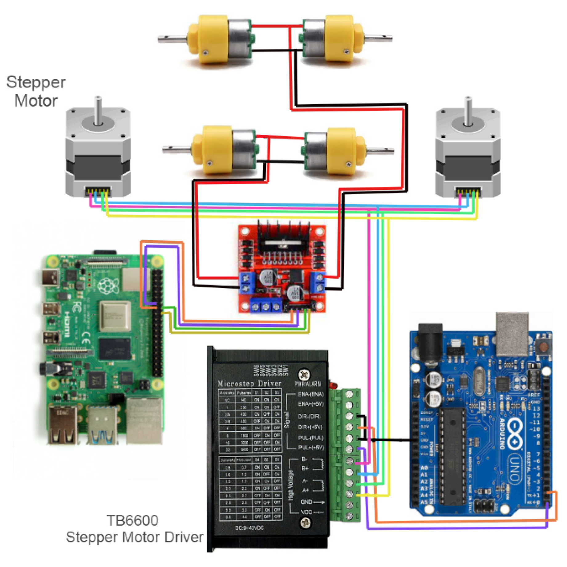
To move the flap, two Geared DC motors were with a rpm (rotation per minute) of 30 and an operating voltage of 9–12 volts and two NEMA17 stepper motors were implemented with step angles of 1.8 degrees and holding torques of 4.2 kg-cm. The two Geared DC motors were attached to each side of the robot, and then each was connected to the DC Stepper motors such that the axes of the two motors were perpendicular to each other. The Geared DC motors were responsible for the vertical movement of the flap, while the Stepper motors were responsible for the extending and retracting motion of the flap. In this setup, the two Geared DC motors were both connected to the second motor port of the second L298N motor driver, while the two DC Stepper motors were controlled with the TB6600 stepper motor driver, which was powered by the second Li-Po battery. Further detailed specifications of the components can be found in
Table A1.
4.2. Bucket
Following the flap motion of sweeping trash into the bucket, the bucket was programmed to empty the trash into the collector bin of the robot. This bucket was rotated with the help of gears, as the load from the weight of the bucket on the motor alone was large enough for it to be lifted. These gears provided an additional mechanical advantage, and the bucket was thus lifted. Once the bucket was lifted, owing to the force of gravity, the trash fell into the bin as desired.
For the gears, a 5:1 ratio was used due to their large mechanical advantage in the output and availability at the time. The load capacity can be calculated by Equation (6).
Since,
where,
T1 = 4 kg-cm (2 kg-cm each) &
d2:
d1 = 5:1.
Therefore, T2 = 20 kg-cm.
Assuming the distance to the center of mass to be around 13 cm, the gear assembly is capable of lifting up to 1.5 kgs of load. The distance to the center of mass can vary as the trash of varying sizes can be picked up, which would affect the load-lifting capability of the robot.
To move the bucket, two DC Geared motors with an rpm of 60 and operating voltage of 9–12 volts were used. One motor was attached to each side of the bucket, and a small gear was attached to the shaft of the motors, which drives the larger gear attached to the shaft of the bucket. Due to this gear setup, lifting heavy objects in the bucket was made possible. These motors were connected to a different L298N motor driver module, but in the same port as they were both required to move at the same time. The motor driver was powered by a separate 2200 mAh Li-Po battery with the same specifications. Further detailed specifications of the components can be found in
Table A1. The connections of the actuators of flap and bucket are shown in
Figure 2.
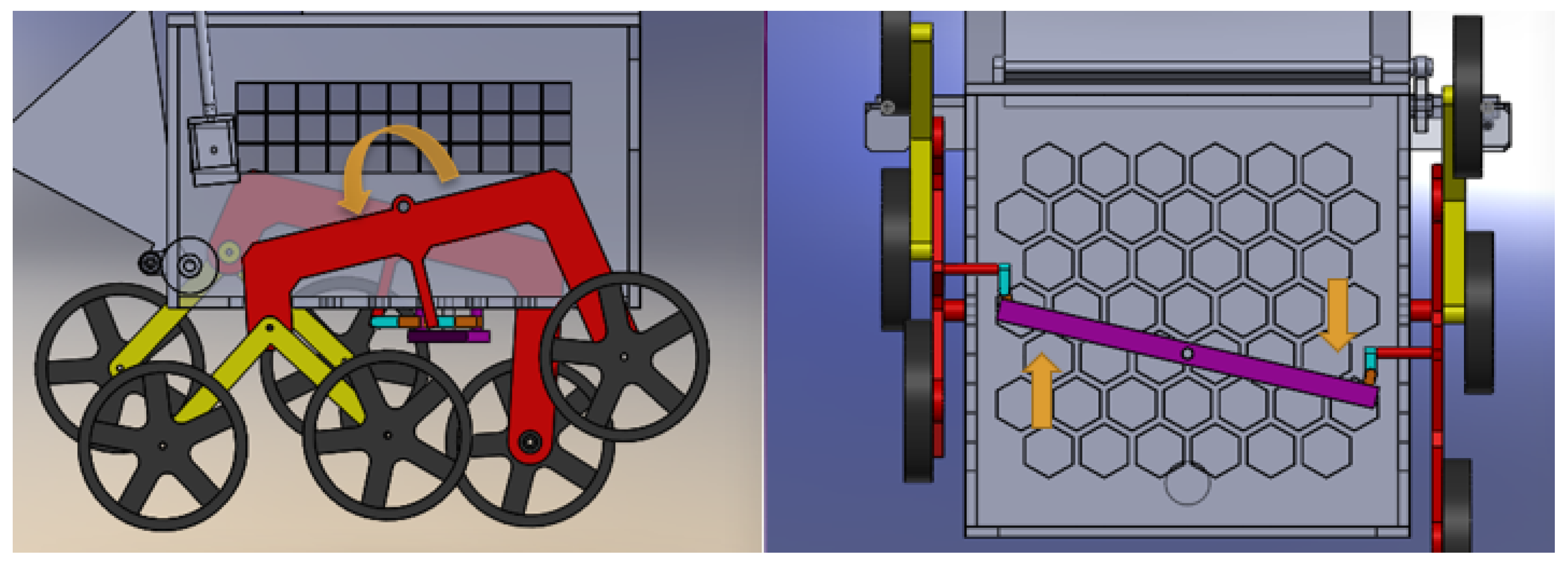
4.3. Rocker-Bogie Mechanism
This mechanism was developed in 1988 by NASA for their rover missions to be able to easily adapt to unknown and rugged terrains. This system principally worked like a suspension system, but without any springs. Using this mechanism, the robot motion on the rough surfaces was made relatively smooth. When the rocker in red on the one side rotated, it either pushed or pulled the differential shaft, which in turn moved the rockers on the other side in the opposite direction. As can be seen in
Figure 3, the rockers were moved in opposite directions when one was moved. The differential shaft was to be restrained within a certain range to maintain the integrity of the structure through the differential limiters [
27].
To drive the robot, around six DC geared motors were implemented (one on each leg of the rocker-bogie mechanism). These motors were connected to the L298N motor driver module. The motor driver was powered by a 2200 mAh Li-Po battery at 11.1 v. The control signals were provided to the motor driver by the Raspberry Pi. The wheel on each side rotated in the same direction in all cases, so they could be connected at the same port of the motor driver. There were four cases in which the motor ran:
All forward—robot moves forward.
All backward—robot moves backward.
Left Forward and Right Backward—robot turns right.
Right Forward and Left Backward—robot turns left.
4.4. Camera Setup
A web camera was placed on top of the robot at a height of 15 cm above the robot’s body to give the camera a better viewing angle (especially when the camera pans) and improve trash-detection capability. Otherwise, the robot’s body would obstruct the view of the ground. The camera was attached to a servo motor to pan the camera in the left-right direction. The camera served as an important sensor for the robot as it was used to detect trash, following the trash by panning the camera with the help of the servo motor. When the trash was not detected, the camera looked actively for the trash, and when the trash was detected, it changed the mode from searching to following and kept the trash in the center of the camera.
To move the camera, a TowerPro SG90 Continuous Rotation 360 Degree Servo Motor with a rated speed of 60 rpm, stall torque of 1.2 kg-cm, and rotational degree of 360 degrees was used. The camera was directly connected to the shaft of the servo motor such that when the motor rotated, a left-right motion was induced in the camera. This servo motor was directly connected to and controlled by the Raspberry Pi board. Further detailed specifications of the components can be found in
Table A1.
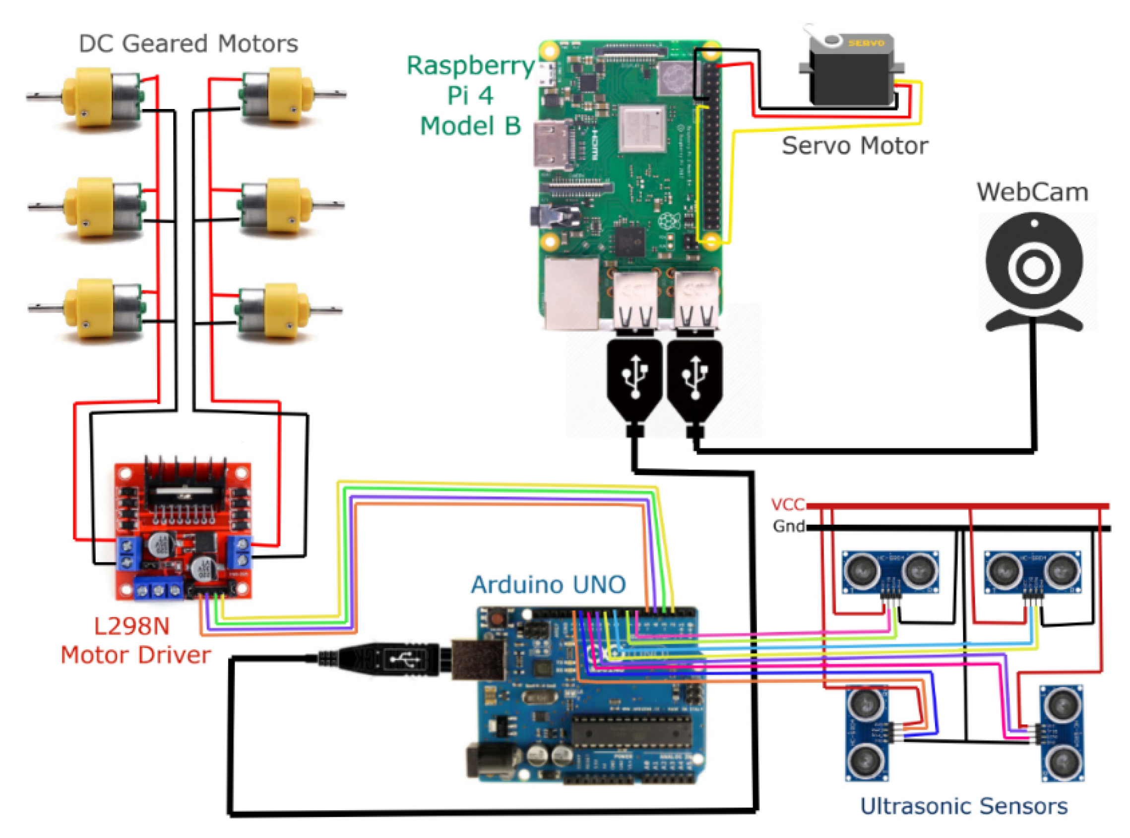
The connections between the actuators, camera and sensors with the microcontrollers are shown in
Figure 4.
4.5. Sensors
Four ultrasonic sensors (two in front and one on each side of the robot) were placed. The two sensors in front were used to detect the trash and stop the robot at the right spot for the flap to sweep the trash, and for obstacle avoidance. The sensors on each side were used to avoid obstacles as well as to circum-navigate around the obstacles as the robot moved towards the trash. A GPS module tracked the robot’s location in real time, which in turn aided in the monitoring of the robot at any given time. This location was important for the path-planning purposes.
5. Object Detection Model
Building an object detection model to detect ‘trash’ specifically can be an exacting task. A polythene bag, a can, coffee cup, toffee wrapper, paper plate, liquor bottle, cardboard piece, plastic bottle, and many other items of varying brands and built materials can be considered as trash. Often, these trash items are not brand new: they could be partially or completely crushed, their paint could be tinted, and their structures worn out, torn, partly broken, faded, rusted, covered with dust, smeared, tarnished, and etc. Moreover, the trash object could be lying upside down on the ground or horizontally, and any angle of this object could be facing the camera fitted on the robot’s roof. The trash-collecting robot might have to carry out these detections at different times of the day and with varying lighting. The background has a key role in such detections and training the object-detection model with a suitable background is beneficial for building a model which can provide accurate detections.
5.1. Data Preparation and Pre-Processing
In this paper, the dataset for the computer vision model was taken from the TACO (Trash Annotations in Context) collection of images. TACO is an open dataset containing about 1500 images of all sorts of non-biodegradable litter in vast variations of backgrounds like on green foliage, beaches, near sidewalks, rocky regions, as well as indoors and at varying times of the day. The resolution of these images ranged from about 2000 to 6000 pixels in each dimension [
28]. Out of these, 310 outdoor images were hand-picked to use in the given application of building the Outdoor Autonomous Trash-Collecting Robot. These images were then cropped into square images. During training, the model resized images to square format, and thereby the cropping of images beforehand facilitated maintaining the aspect ratio. Images reduced to 300 × 300 pixels before inputting into the model fastened the process of training and enabled less load on the processor.
LabelImg, an image annotation tool, was incorporated for manually annotating the selected images. Bounding boxes were made on all the objects which were considered as litter on each image for a single class, namely ‘Trash’, to be used in the custom model. The image annotations contained x-y coordinate information regarding the ‘trash’ locations in each image. They were saved in both YOLO format, as .txt files, as well as in the PASCAL VOC format, as .xml files. Annotating images was a necessary step, without which the use of a weakly supervised model was the only resort. The dataset was then split into a 10% test set and a 90% train set, out of which the training set contained 277 images and the test set contained 30 images.
5.2. Model Selection and Model Structure
There were multiple deep-learning object-detection models, for example, SSD-MobileNet, RCNN, and different versions of YOLO, to name a few. All these models principally were convolutional neural networks (CNNs) [
29]. The models that were experimented on in the current article for the purpose of trash detection for inculcation in the autonomous outdoor Trash-Collecting Robot were Mask-RCNN, YOLOv4, and YOLOv4-tiny, respectively. Mask-RCNN is an extension of faster-RCNN.
In Mask-RCNN, there was a backbone of deep convolutional neural networks, following which a region proposal network (RPN) and RoIAlign together provided region CNN features. These features finally were computed in a Box offset regressor, Softmax classifier, and Mask FCN predictor to produce the end results of bounding box, object classification, and the image segmentation [
30].
The loss function for Mask-RCNN is calculated as shown in (7), where
Lcls stands for losses in classification,
Lbox stands for losses in bounding box regression, and
Lmask stands for losses in mask prediction. The overall loss function of Mask-RCNN is similar to that of Faster-RCNN, the only difference being those losses due to mask (
Lmask) were additional.
Pi is the predicted probability and
Ncls is the factor by which the loss function is normalized.
R is a robust
L1 loss and
ti for
i belongs to {
x,
y,
w,
h} is the position and dimension parameters of the bounding box
The dimension of mask for every RoI (Region of Interest) is
m∗
m and
yij is the ground truth table, i.e., 1 or 0 in cell (
i, j) and
ykij is the probability that is predicted for the
kth class [
31].
YOLO (You Only Look Once) belonged to the family of one-stage detectors, unlike the RCNN, which belonged to two-stage detectors. YOLO performed bounding box regression and classification at the same time as a single convolutional network was run on the image. In the present paper, the base network that was used in the Mask-RCNN deep-learning model was Resnet-101 and the base network used in YOLOv4 and YOLOv4-tiny was CSPDarkNet53. In YOLO, the input image is divided into a S∗S grid. Each cell of this grid is responsible for contributing to the bounding box predictions and the scores for those boxes as well. The non-max suppression technique is used to fix the issue of multiple detections by discarding the boxes with lower probabilities [
32]. In YOLOv3, DarkNet53 was used [
33], whereas in YOLOv4 the superior learning ability of the CSPnet (Cross Stage Partial network) was implemented by using CSPDarkNet53. The activation function used in YOLOv4 was ‘mish’. YOLOv4 used a DropBlock regularization, mosaic data augmentation method, Cross mini-Batch Normalization (CmBN), and self-adversarial-training (SAT), which were all new features compared with its previous versions. Moreover, Complete Intersection over Union loss (CIoU loss) was applied as well [
34].
YOLOv4-tiny is a compact version of YOLOv4. YOLOv4-tiny is known for its much faster training and detection ability, making it beneficial for development on mobile and embedded devices. YOLOv4 has three YOLO heads, whereas YOLOv4-tiny has only two. The activation functions used in YOLOv4-tiny are leaky and linear. YOLOv4 was trained from the weights of 137 pre-trained convolutional layers, while YOLOv4-tiny from 29 pre-trained convolutional layers.
The loss functions for YOLOv4 and YOLOv4-tiny are given below:
The localization loss measures the errors between the predicted boundary box and the ground truth of the locations and sizes. The localization loss is based on CIoU (Complete Intersection over Union) loss. CIoU simultaneously considers the overlapping area, the distance between center points, and the aspect ratio. To count the box responsible for detecting the object, the function is given in (12).
where:
is the Euclidean distance (
d),
c is the diagonal distance of the closure.
where,
w and
h are the width and height of the box.
Confidence loss is the measure of the objectness of the box. The function is given as in (16):
where:
is the box confidence score of the box
j in cell
i,
denotes that the
jth bounding box predictor in cell
i is “responsible” for that prediction. It is also a complacent for
.
Most boxes do not contain any detectable objects. This can cause class imbalance problems, which means that the model is trained to detect background more rather than detecting the objects. To counter it, a factor λnoobj (default: 0.5) is added to weigh it down.
Once an object is detected, the loss due to overlap between the classes can be calculated mathematically as the classification loss at each cell is given by the squared error of the class conditional probabilities for each class, as shown in (17).
where,
is the conditional class probability for class c in cell
i [
35].
5.3. Training and Hyperparameter Tuning
The technique of transfer learning was implemented. In transfer learning, a model pre-trained on a large image classification dataset, for example ImageNet or the MS COCO (Microsoft Common Objects in Context) dataset, could be customized to perform a given task. The ImageNet dataset is a much larger dataset with a whopping 14 million plus images, approximately, while the MS COCO has only 328 K images. Though ImageNet is a better option for the computer vision model, the computational power at disposal must be considered. In this study, weights of models pre-trained on the MS COCO dataset were used. The convolutional neural network base of the pretrained model was frozen so as to be used as a feature extractor while the top few layers, i.e., the head, were trained on the ‘Trash’ dataset for the purpose of performing the specific classification. The learning rate of this new, desired object-recognition-training dataset was kept low, at 0.001 initially. This was done so that small updates to the weights were made during the training, which avoided undesirable divergent behavior in the loss function. Transfer learning indefinitely increased the effectiveness of the model by producing much more accurate results, since here the model was not trained from scratch; instead, some pretrained weights were used. The impediment due to the small dataset was overcome through this technique as well. The intersection over union (IoU) threshold was used to determine Average Precision (AP) being 0.5% or 50% for all three of the models. The Mask-RCNN model was trained for 25 epochs, where the number of training steps per epoch was set to 277, which was also the number of images in the training set. The YOLOv4 model was trained for one epoch and was given a batch size of 64 and the max_batches parameter was set to 2000 since the model was used to detect a single class.
5.4. Challenges in Implementation and Its Possible Solutions
A very large number of appropriate pertinent images were required to be trained to be suited for practical implementation in real-world scenarios. These images were additionally required to be annotated images, and otherwise needed to be manually annotated by a human, which was laborious. By increasing the training-set size, the training time too proportionally increased, and higher computational power was required. If one wished to commercialize the product, then to increase the computing power for training of the deep-learning model, some cloud services like AWS, IBM, etc., using multiple GPUs at one time, could be used. Companies may wish to invest in them, as most of those services are paid for depending on the number of use-hours and how much of their computing power and other tools are used.
Moreover, the Coral USB Accelerator could be used in Raspberry Pi, as it increases the processing capacity of the Raspberry Pi and thereby also decreases the object detection time drastically.
6. Implementation and Operation of the Robot
6.1. Object-Detection Model Preparation for Raspberry Pi
The trained deep-learning model weights were saved in Hierarchical Data Format (HDF), i.e., as an h5 file. The files in this format, or h5 files, occupy much less memory than pickle files. The saved model was converted into a TensorflowLite model to make it feasible for running in embedded systems like Raspberry Pi.
6.2. Robot Locating and Workspace Definition
Before the robot was switched on, four coordinates were needed to be input in the Raspberry Pi to define the working area of the robot. The four coordinates represented the four corners of a rectangular box. When the robot got out of this box, the robot turned around to return to the workspace. This was carried out by calculating the normal distance from the lines to the location robot with the help of the GPS module.
6.3. Robot Path-Planning
After entering the previously mentioned coordinates, when the robot was switched on, it roamed around inside its workspace and searched for any trash through the camera while also avoiding any obstacle with the help of the ultrasonic sensors placed on its front and sides. When the robot detected garbage, it made a box around the trash. The centroid of this box was calculated and then it compared the position of the centroid with respect to the x and y axis of the frame. In any case, if the robot detected multiple trash boxes in a single frame, it then chose the box whose centroid was closer to the left side of the frame.
When any obstacles were detected, the robot would stop for 2 s and check again if the path was still blocked. If the path was not blocked, the robot continued on its path. However, if the path was still blocked, the robot would generate a random angle and turn to match that angle with the help of the magnetometer sensor module. Since the generated angle would be random each time, the robot followed a random path and covered the entirety of the defined workspace. As the robot did not need to cover each point, this method should suffice the needs of the robot in the coverage to detect any trash through the camera. The robot turned such that the angle of the servo motor controlling the camera became 90 degrees, i.e., the robot, camera, and servo were aligned in the direction of the trash. The robot started moving towards the trash and maintained the trash in the center of the frame of the camera by moving the wheels and changing its direction accordingly. If the robot encountered an obstacle during trash following, it could simply move over it thanks to the Rocker-Bogie mechanism, which allowed it to climb over obstacles twice the size of its wheel’s diameter.
If any obstacle blocked the view of the trash for the robot that may have been placed after the trash was detected by the robot, the robot did a couple of things. Firstly, the servo motor attached to the camera started to move to keep the trash in the frame and allowed the robot to turn. Furthermore, the robot turned either left (default) or right according to the input from the sensors. After turning (say, left), the robot started to circum-navigate while maintaining a certain distance from the obstacle with the help of the right ultrasonic sensor. The robot continued to circumnavigate till the angle of the servo and the robot coincided again, after which the robot left the obstacle and continued moving towards the trash.
When the robot reached the trash, the two ultrasonic sensors on the front returned TRUE and made the robot stop. The bucket rotated to touch the ground. Next, the flap unfolded and swept the trash into the bucket. The flap then folded and went back to its default position, after which the bucket rose to roll the trash in the bin. This concluded in the trash pick-up activity being completed, and thereafter the robot began searching for more trash again.
6.4. Monitoring of Collector Bin
When the bin of the robot filled up with trash, IR sensors inside the collector bin gave the signals to the microcontroller. Then, the robot moved to the predesignated location and switched itself off. The location was to be initially fed to the robot and must be inside of the box created by the four coordinates.
7. Simulation on Various Terrains
The SOLIDWORKS Motion tool was used to perform a motion analysis of the robot when it encountered any obstacle in its path. The motion was simulated over various terrains of different shapes and sizes to test its limits.
Table 2 shows screenshots from the simulation run. The simulation run video can be found in the
supplementary files.
The robot easily overcame the rise in the terrain of the size of the wheel’s diameter. The flexibility granted through the Rocker-Bogie mechanism allowed the robot to remain stable with all wheels grounded even when the terrain on each side of the robot was at different levels.
8. Results and Discussion
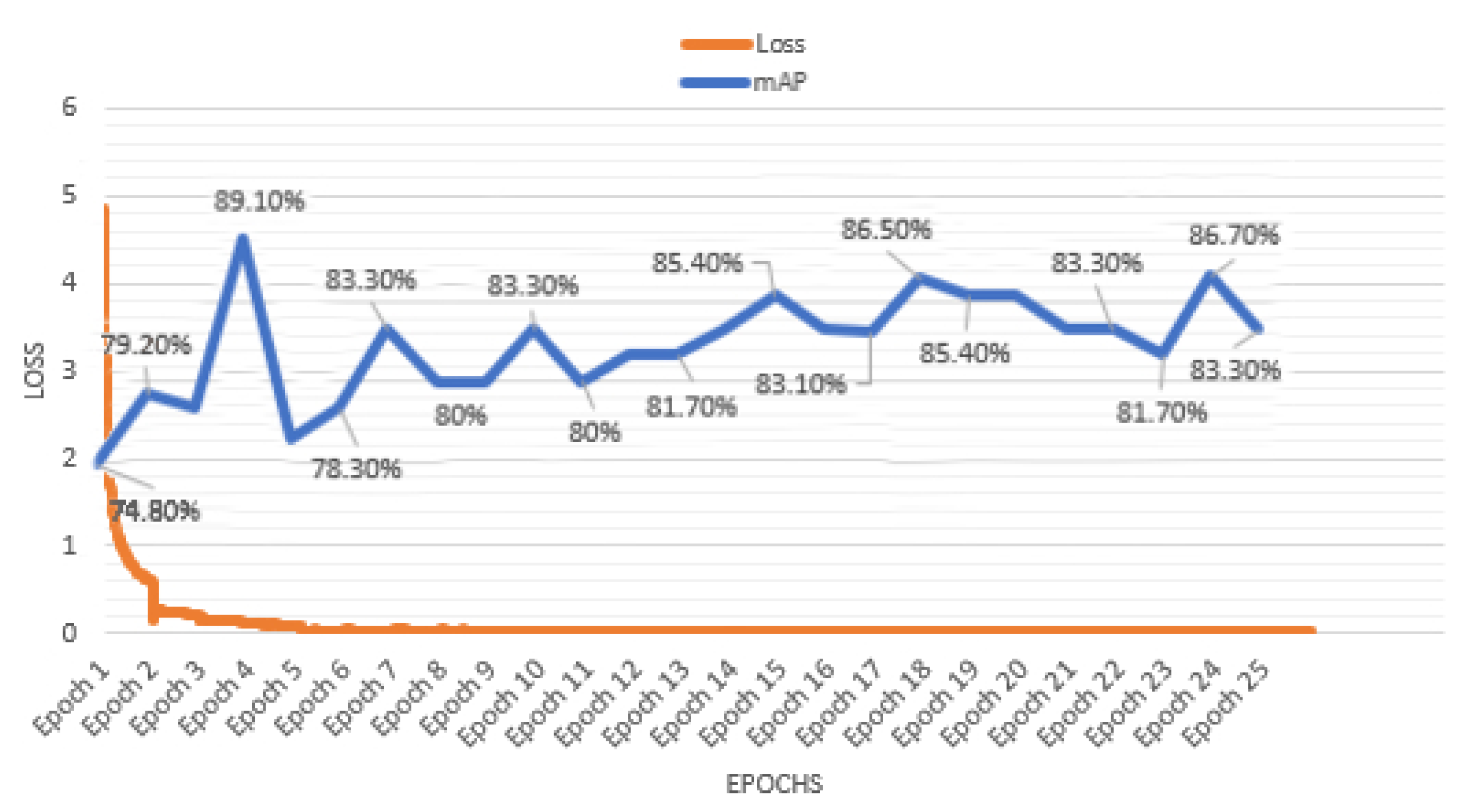
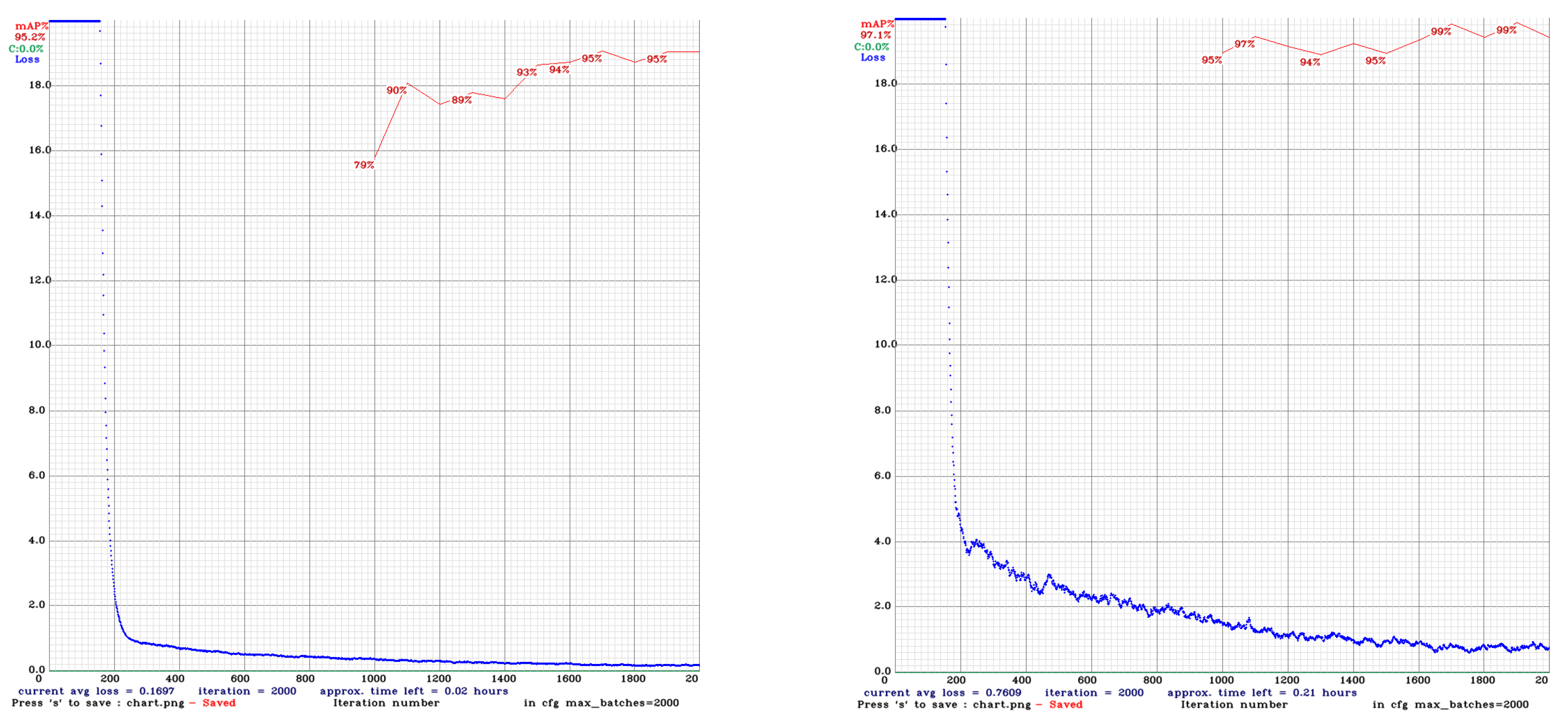
The decrease in losses as shown in
Figure 5 and
Figure 6 is an indication of increase in the confidence level of the model predictions with increase in training. All the three models displayed a steep decline in the losses in the initial training period itself, after which it continued to decline gradually. In MaskRCNN, the final loss obtained at the end of training for 25 epochs was 0.0282. In YOLOv4, the final average loss obtained after a total of 2000 iterations was 0.7609, whereas the final average loss in YOLOv4-tiny was 0.1696. While training in the three models, the mAP followed a trend of increasing with some small decreases along the way. Mask-RCNN demonstrated major upside in the mAP in the 4th epoch, YOLOv4 in the approximately 1500th iteration, and YOLOv4-tiny in the iteration around 1500. YOLOv4 showed an overall rise in mAP; YOLOv4-tiny showed a slight overall increase in mAP.
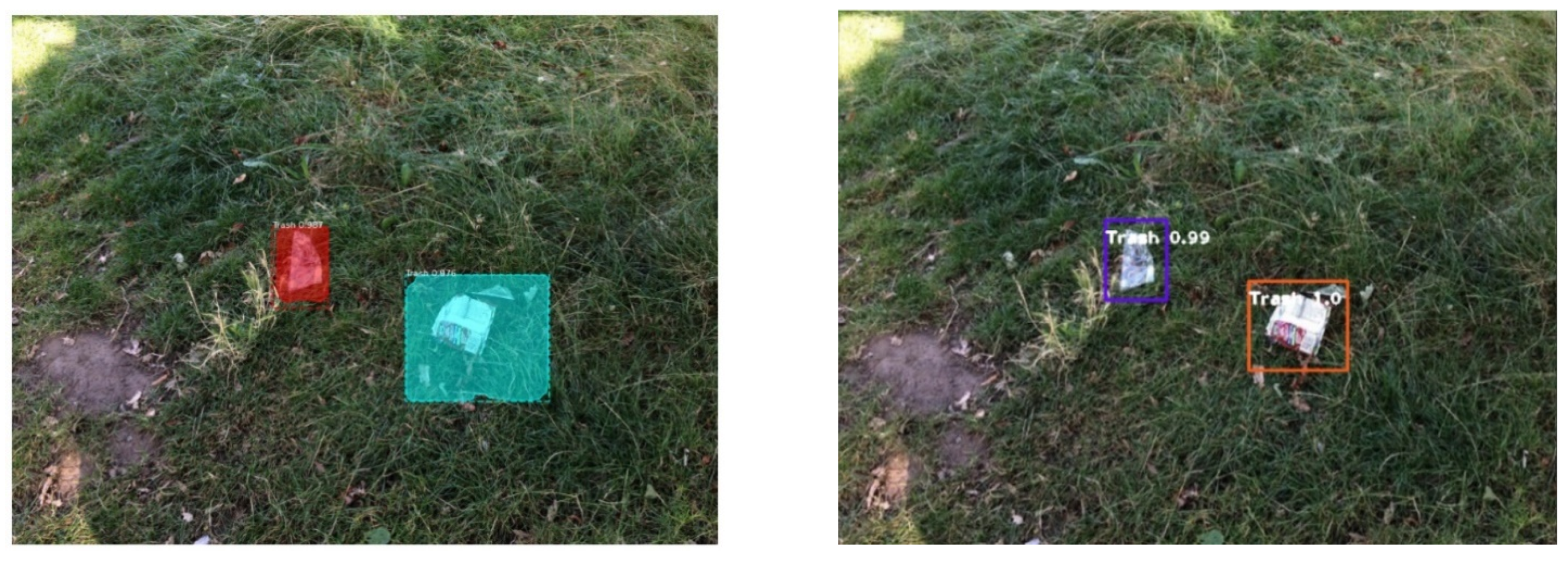
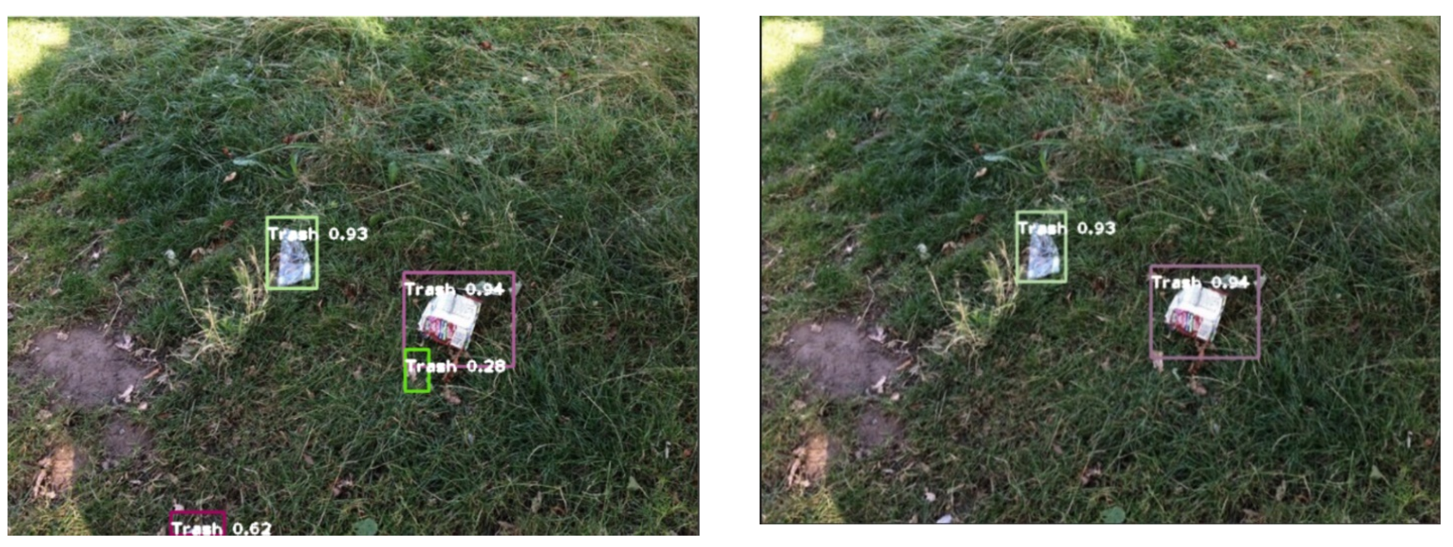
Figure 7 shows the detection using MaskRCNN model and the YOLOv4 model. Whereas, in
Figure 8 shows the detection using YOLOv4-tiny model.
The YOLOv4 and YOLOv4-tiny had a much faster inference time in comparison with Mask-RCNN.
Table 3 provides a clear outline of the best mAP and the respective inference time that was achieved for each of those models. These detection speeds were obtained when testing using a GPU NVIDIA GeForce GTX1650 on the computer.
The inference times were noted after testing for various resolution images containing different numbers of trash items, and not much variation was observed in terms of inference time when tested using the same model. The average of three inference time values for each model was calculated and written in
Table 3 for analysis and comparison with other models. Although YOLOv4 attained the highest mAP, YOLOv4-tiny attained the highest detection speed. For autonomous trash-collecting robots which have to make on-the-spot decisions, swiftness in detections is paramount and thereby YOLOv4-tiny was an apt model, since even accuracy was not compromised much.
Once the training of the model was completed on the laptop, it was ported to the Raspberry Pi. Based on the frame rate (frames per second), the Raspberry Pi was able to use the trained model at 12% (8.34 times slower) than the computer.
The YOLO models performed faster detections than Mask-RCNN, since these models are single-shot detectors, in contrast to the RCNN family, which performs two-shot detection. Furthermore, between the two YOLO models used, YOLOv4-tiny produced faster results as compared with YOLOv4 since it has a much lighter architecture. YOLOv4-tiny was thus incorporated in this project where the software portion was required to give quick results for the robot to work in a comprehensive manner. The model worked decently in the real-world tests. The fps was capped at 20 frames per second to ensure consistent performance on the Raspberry Pi 4b.
The path-planning algorithm adopted made the robot work in an endless loop where the robot searched, detected, and picked up the trash [
36]. This loop can be bounded by time where a specific duration can be picked for the robot to work. An emergency stop button can be placed on the robot as well such that the program monitor could stop the robot due to unforeseen events.
9. Conclusions
A unique robot was built from scratch to autonomously collect trash from public areas. The robust mechanism allowed the robot to pick up trash of varying sizes from different types of surfaces. The robot was capable of traveling, avoiding any obstacles, and searching for trash with the help of the sensors and image-processing on the camera feed. A comparative analysis among MaskRCNN, YOLOv4, and YOLOv4-tiny computer vision models was carried out. The graph for loss and mAP while training was obtained, which provided in-depth insights regarding how the loss and mAP varied with more training of the model. The experimental results revealed that YOLOv4 was able to achieve the highest mAP (mean Average Precision), while YOLOv4-tiny, owing to its light nature, produced the fastest inference time. The final model classified all the trash objects present in the given frame accurately as ‘Trash’, along with the object localization and confidence level of the detected object or objects. Once the trash was detected, the robot was adept at reaching the trash and picking it up while avoiding any obstacle that may have been in the way by using the circum-navigation technique. In the future, we will produce a prototype and test the system with more datasets within a university campus.
For further improvements in this project, several features could be added. Once the non-biodegradable garbage was collected, garbage segregation could be separated into categories/classes like glass, metal, plastic, cardboard, paper, and etc. so that, accordingly, the decision between applying pressure at all and applying proportional pressure to the material strength to compress the item could be taken so as to enable easy recycling, and more garbage could be collected by the robot at a time before every unload. In addition, all types of wastes could be programmed to be collected, i.e., both biodegradable and non-biodegradable, and thereafter additional segregation could be performed if feasible. The incorporation of the advanced technology of self-charging into the autonomous robot was an additional favorable attribute. The deep-learning model could be trained more while keeping overfitting in check and on a substantial dataset. It could be programmed to perform additional software computations for the detection of moving obstacles like people, animals, and vehicles, making it more prepared for unforeseen circumstances. Reinforcement learning is another method which could be considered for implementation in the future versions of this robot where the robot learns on its own from its surrounding environment, develops intelligence, and grows capable of making better intuitive decisions with more exposure and experiences. The front and rear wheels of the robot can be turned on their axes to steer the robot in any direction while staying in the same place. The trajectory of the robot can be tracked to increase the efficiency of the robot by avoiding multiple visits to the same area and rather moving to other areas [
37].


 ,
, 


