A Comprehensive Analysis of Deep Neural-Based Cerebral Microbleeds Detection System

Abstract

Machine learning-based systems are gaining interest in the field of medicine, mostly in medical imaging and diagnosis. In this paper, we address the problem of automatic cerebral microbleeds (CMB) detection in magnetic resonance images. It is challenging due to difficulty in distinguishing a true CMB from its mimics, however, if successfully solved, it would streamline the radiologists work. To deal with this complex three-dimensional problem, we propose a machine learning approach based on a 2D Faster RCNN network. We aimed to achieve a reliable system, i.e., with balanced sensitivity and precision. Therefore, we have researched and analysed, among others, impact of the way the training data are provided to the system, their pre-processing, the choice of model and its structure, and also the ways of regularisation. Furthermore, we also carefully analysed the network predictions and proposed an algorithm for its post-processing. The proposed approach enabled for obtaining high precision (89.74%), sensitivity (92.62%), and F1 score (90.84%). The paper presents the main challenges connected with automatic cerebral microbleeds detection, its deep analysis and developed system. The conducted research may significantly contribute to automatic medical diagnosis.

1. Introduction

The number of successful applications of machine learning algorithms is constantly growing. Unlike classic approaches, deep neural networks (DNNs) are naturally predisposed to efficiently handle vast amounts of data. They successfully cope with inaccurate or noisy data, different sizes and orientations of objects, as well as, varying lighting conditions. Moreover, if these algorithms are properly selected and trained, they have a high capacity to generalise the acquired knowledge. The latter is extremely important in practical applications where we have to struggle with a variety of cases, small, yet significant differences between classes, and a large diversity of objects within a class or an insufficient number of appropriately labelled unbalanced data.

This paper approached the very important problem of cerebral microbleeds (CMB) detection in MR images. Cerebral microbleeds are small, oval, hypointense areas visible at T2*-weighted or susceptibility-weighted (SW) imaging [1,2]. The cerebral microbleeds can be seen in the images due to changes in local magnetic susceptibility because of pathologic iron accumulation as a result of (most often) perivascular macrophages due to vasculopathy. A single microbleed is mostly from 2 to 5 mm or even 10 mm in diameter [3]. However, the size is not the differentiation criterion, as it can be deceptively increased due to blooming artifacts. MR images give a detailed three-dimensional view of organs and can be effectively used to detect and analyse the abnormalities in them. Nonetheless, automated detection and classification of brain lesions, in particular CMBs, in 3D MR images is a challenging task due to their wide distribution within the brain, small sizes compared with the whole image, and the similarity between different lesions and lesion mimics.

The paper is organised as follows: further, in this section, we present the medical aspect of cerebral microbleeds as well as related works regarding CMB detection and challenges in this field; in Section 2, we introduce the reader to the case study, our approach including algorithms and data handling, while in Section 3, we describe conducted experiments and deliver the results. Finally, in Section 4, we discuss obtained results and conclude them in Section 5.

1.1. Cerebral Microbleeds—Fundamentals

Cerebral microbleeds are small, chronic brain haemorrhages that are caused by several different pathological processes in the small, cerebral vessels [4,5,6].

According to [7], around 5% of the healthy population has microbleeds, but their higher occurrence may be connected with several medical conditions. The presence of CMBs is strongly correlated with cognitive dysfunction [8]. Moreover, it increases the risk of stroke recurrence [9]. However, CMBs can also be found in healthy elderly people with unknown clinical implications [9].

The most commonly used method for the detection of CMBs is Magnetic Resonance Imaging (MRI) [10]. This method uses a non-ionizing radiation method to create diagnostic images. The image is created thanks to the natural magnetic properties of tissues. Specifically for detection of CMBs neuroimaging in MRI include T2* sequence or susceptibility-weighted imaging (SWI) [1,2]. Cerebral microbleeds appear on MR images as spherical signal loss (hypointense focal area), due to the paramagnetic properties of hemosiderin. CMBs as hemosiderin deposits contained macrophages that are displayed as hypointense images, which is related to containing high concentrations of iron. Paramagnetic properties of hemosiderin cause a signal loss because of susceptibility effects [11,12]. Detection of CMBs is increasing with the frequency of usage of MRI for diagnostic, CMBs are accidentally found along with different diagnostic pathologies.

Detection of all present cerebral microbleeds in MRI is crucial for proper diagnosis and treatment, as it is a common abnormality connected with different diseases. Despite increasing detection, there is still a lack of clear guidance and quick detection of CMB. The process of manual inspection and detection of microbleeds is very laborious and time-consuming. Automating the whole process of CMBs detection would make radiologists’ work easier and faster.

1.2. Problem Statement and Related Works

The problem of CMB detection has been considered in a number of publications in recent years. Based on their analysis, several important challenges and conclusions regarding data, approaches and algorithms can be indicated.

Despite the great success of ML-based systems in the medical field, which outperforms other classic methods, there are many problems related to the use of algorithms. Among others: insufficient number of publicly available, labelled datasets; different quality and resolution of data; uneven class balance within the datasets; still poor ability to generalise results in some cases; and inconsistent evaluation of results, hindering their analysis [13,14,15,16,17,18,19,20].

In this paper, we try to discuss and find a solution to some of them in the case of CMB detection. Our extensive analysis and experiments were conducted to propose a way of synthesis the suitable DNN-based system for reliable CMB detection, which shows high performance and generalisation ability.

The problem of data shortage is common in the analysis of medical data. In radiology, class annotations alone are hardly enough for most prediction tasks. CMB similarly requires manually annotated bounding boxes or segmentation masks, which have to be done by medical experts. Such a precise manual data annotation is not only expensive and time-consuming, but also requires data anonymisation, and still, the CMBs are labelled only by a single point. Mostly, new datasets are created for specific research carried out by research teams. They are not later published due to complicated privacy regulations.

Moreover, existing datasets are prepared by different groups with different measurement equipment, medical procedures and also, for different purposes (e.g., strictly for the needs of physicians, data analysts, ML specialists). For instance, there are differences between the labelling methodology or the examination parameters. Not only the MRI machines specification depends on their producer, but also during the MRI examination technician set parameters depending on a case. The differences between patient origin are also crucial, as the human anatomical structure is different.

Therefore, although datasets seem similar, especially for non-specialists in the medical field, to design a data-driven decision-support system able to efficiently operate in very different conditions, it is essential to have scans as diversified as possible.

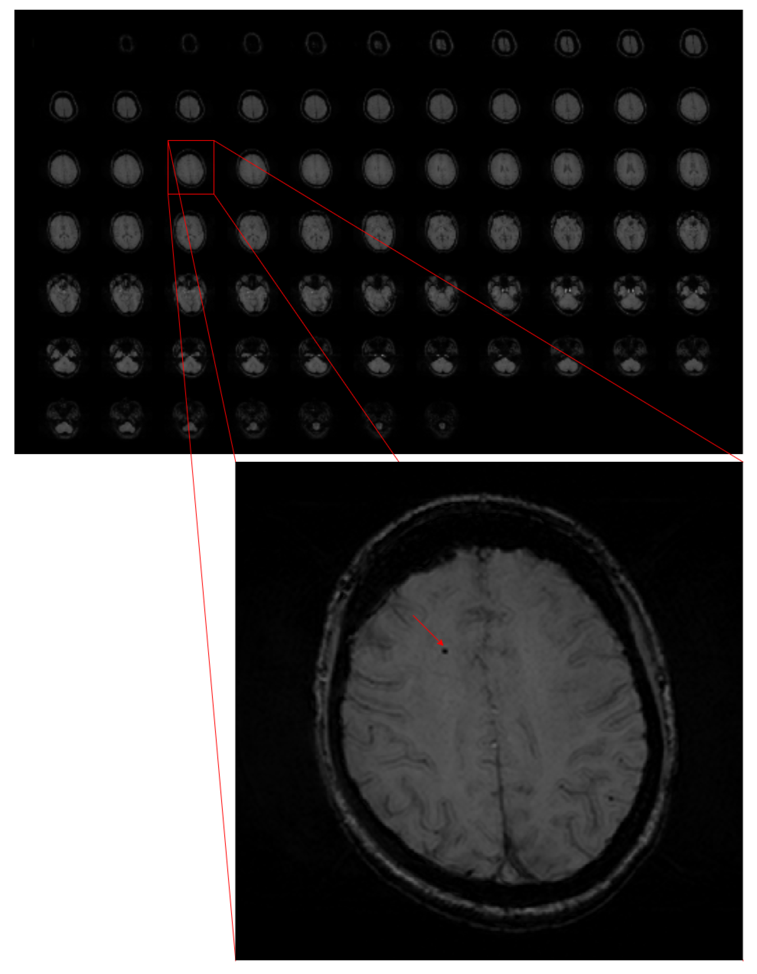
In the case of automatic detection systems, it is fairly easy to mistake microbleeds with other objects, mainly because of their small size compared to the whole image, their similarity to the background, and lesion mimics (see Figure 1). For instance, an oval cross-section through a vessel or calcification is very similar to a CMB. The differences between microbleeds and other objects can be observed when rating the whole MRI altogether.

Sometimes, it is difficult to objectively compare the research results because, as mentioned earlier, there is a lack of objective benchmark databases. Besides, different metrics are used to evaluate the systems. For example, sensitivity is sometimes the only metric reported. However, it is relatively easy to obtain high sensitivity scores, but at the price of a large number of false positives. To avoid this, other metrics should also be provided—for instance, precision or FPavg (average number of false positives per subject). Of course, the goal is to have as high sensitivity as possible with a low false-positives score.

The development of ML methods has caused that traditional methods of image processing and analysis have been replaced by methods using mainly different types of tools based on deep neural networks.

Generally, ML-based solutions for object detection tasks may be divided into two groups: one-stage and two-stage detectors. In one-stage detectors, both detecting an object and assigning it to the predefined class are done at the same time, while in the two-stage approach, these two sub-tasks are carried out separately by producing the regions of interest (RoI) and then its classification.

The most popular representative of the one-stage approach is the family of YOLO (You Only Look Once) networks, the most recent ones are YOLOv4 [21], scaled YOLO [22] and YOLOv5 [23]. Although such approaches are much faster than two-stage ones, they produce a larger number of false positives and have significantly worse results for detecting small objects. This problem is clearly visible in the work [24]. The YOLO detector produces dozens of false-positive CMBs for one subject; hence, another stage is needed to reduce them.

Although new and better architectures are emerging, such as EfficientDet [25] and Vision Transformer [26], the above-mentioned issues related to the one-step approach have not been diminished.

The most popular architecture from the family of two-stage detectors is R-CNN [27,28] and its successors. The idea was based on defining regions of the proposal using selective search [29]. Then, scale them to a fixed size and apply them to a CNN network for feature extraction and finally to assign them the proper category using a linear SVM classifier. The biggest issue in this approach was the detection speed. Although computational capabilities continue to grow, creating more efficient algorithms makes them more usable in everyday life.

This led to an improvement called Fast R-CNN [30] combining RCNN with Spatial Pyramid Pooling Network (SPPNet) [31] that did not require the fixed size of the region of the proposal passed to CNN.

Another proposed solution to speed up the computation process was Faster RCNN [32]. The novelty was in the generation of regions of interest by applying the Region Proposal Network (RPN). The interesting proposal was Feature Pyramid Networks (FPN) [33] enabling usage of the whole CNN network, instead of just its top layer for the detection task. That enabled achieving significantly better results. These days, the mentioned architecture is often used in object detection problems with different backbone variants.

Regarding the detection of microbleeds, we can generally distinguish between two approaches, two-dimensional (2D) [34,35] and three-dimensional (3D) [36,37,38]. However, three-dimensional convolutional networks have significantly more parameters. For instance, 2D ResNet-50 has 23.9M parameters, while 3D ResNet-50 46.4M has almost twice as much [39]. That leads to high computational costs, without a significant improvement in sensitivity and precision.

Most of the proposed methods were based on a two-stage approach [24,36,37,40]. The first stage aimed to detect CMB candidates and was implemented in different ways, not always using neural networks; for example, the authors of [37,40] used fast radial symmetry transform (FRST). As a result, at this stage, it was possible to detect CMBs with high sensitivity, but the price for that is an enormous number of false-positives, which should be reduced in the next stage.

The challenge in 2D cerebral microbleeds detection is the fact that CMBs are mistaken with objects, like vessels, which are similar in two-dimensional space. The features to effectively distinguish CMBs from CMB mimics become apparent when analysing the sequence of adjacent slices and different types of images from the SWI sequence. Although cerebral microbleeds are best visible in the SWI, other ones also can be used to detect CMB. While most authors [34,35,36,37,40] used only SWI, others used also Phase [24], GRE [41,42], or QSM [43]. The results reported in these papers and a comparison with our approach can be found in Section 4.

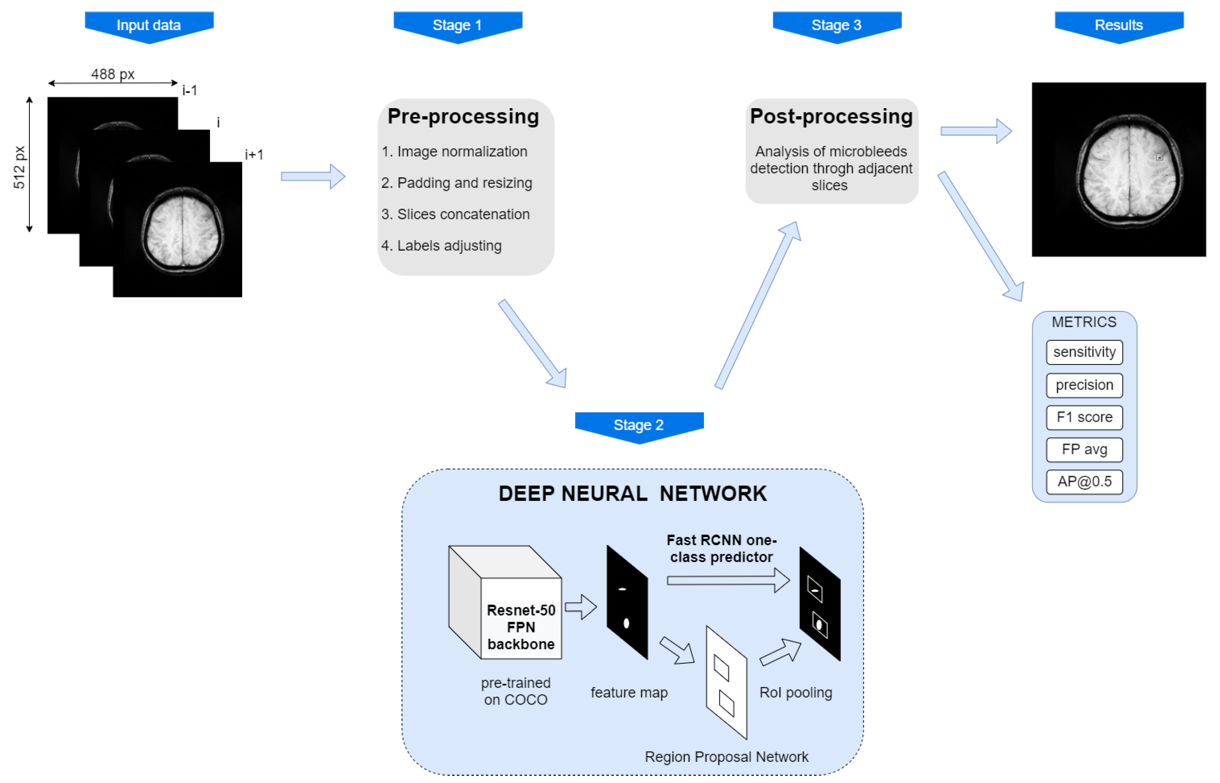
In this paper, we present the results of our efforts put into the synthesis of a cerebral microbleeds detection system. We aimed to achieve a reliable system, i.e., one characterised by both high sensitivity and precision. Therefore, we have researched and analysed, among others, the impact of the way the training data are provided to the system, their resolution, the way of input images pre-processing, the choice of model and its structure, and also the ways of regularisation. Finally, we proposed a new algorithm for the system’s predictions post-processing, which enabled us to partially take into account the three-dimensional nature of the analysed problem, despite using a 2D detector.

The results of the most interesting research are presented in Tables 3–7. The system with the most suitable structure was compared with the results reported by other research groups (see Table 8). Its performance was also tested on a different dataset, completely different from the data used to train, validate and test the system (see Table 7).

2. Materials and Methods

Although the most valuable feature of ML-based systems is their ability to efficiently extract knowledge directly from data, to make the system effective and reliable, it is crucial to provide a sufficient number of representative and well-pre-processed data selections, suitable model and accompanying learning algorithms, and finally, draw appropriate conclusions from the achieved results. In Figure 2, a pipeline illustrating the steps of the synthesis of the proposed system is shown. In the following section, they are described in detail.

2.1. Datasets

During the research, we took advantage of the cerebral microbleeds dataset collected and prepared by Medical Imaging LABoratory (MILAB) at Yonsei University and Gachon University Gil Medical Center [24]. The dataset, along with the ground-truth labels, was prepared by expert neuroradiologists using the pre-processed SWI, Phase and Magnitude images following the gold standard labelling. The details of the data annotation procedure can be found in [44].

The dataset consists of two types of MRI images:

• High in-plane resolution (HR_data): 0.5 × 0.5 mm²;
• Low in-plane resolution (LR_data): 0.8 × 0.8 mm².

The exact parameters describing the images within the dataset are gathered in

Table 1. Summary of data parameters.

Parameter	Shortcut	HR_Data	LR_Data	test_Data	Unit
subjects	-	72	107	20	-
number of labels	-	188	572	78	-
repetition time	TR	27	40	17	ms
echo time	TE	20	13.7	24	ms
flip angle	FA	15	15	-	${}^{\circ }$
pixel bandwidth	BW	120	120	- Hz/pixel
image matrix size	-	512 × 488 × 72	288 × 252 × 72	512 × 512 × 150	voxels
slice thickness	-	2	2	2	mm
slice spacing	-	-	-	1	mm
field of view	FOV	256 × 224	201 × 229	230 × 230	mm2
scan time	-	4.45	1.62	-	min

. For each subject, there are three types of sequences—SWI, Phase and Magnitude, as well as corresponding labels containing a number of slices and coordinates of a microbleed. Although microbleeds are usually visible on more than one slice, the labels do not always relate to all slices where the given microbleed is visible. To test the generalisation abilities of our system, we also used another dataset [36]. This dataset was used only for testing purposes (see Table 1). Its in-plane resolution is similar to HR_data—0.45 × 0.45 mm². This dataset was built for work [36], and it consists of 320 subjects, but only 20 of them are publicly available. Nevertheless, such a batch of data collected in other conditions than data used for training and evaluation of the proposed system, used just for testing, ensures higher confidence of obtained results evaluation.

2.2. Data Pre-Processing

It is well known that proper data pre-processing has an important influence on the capability to properly train a model. In this case, the pre-processing stage involved a few steps.

We resized images to select the appropriate size of the input images and then to scale them accordingly. Based on the number of experiments we decided to utilise images of a size: 512 × 512 (or 288 × 288 in the case of LR_data). The content of medical data (e.g., regarding the images shape, size, colour, contrast, etc.) is of great importance for analysis, and therefore should be modified very carefully, if needed. In particular, the aspect ratio of the images should not be changed because it might deform the lesions in the original images. We first pad all images to square size. This way, any further resize will not deform the lesions. The influence of image size on the final results was also the subject of research (see Section 3.3).

Next, the data were normalised and standardised by reducing the value of a single pixel by the image mean and dividing it by the image standard deviation.

As it was aforementioned in the text, microbleeds may be easily mistaken with vessels or other objects visible in the image. To distinguish CMB from its mimics, analysis of few adjacent slices is essential. It is possible through the 3D sequence; however, in our case, we use 2D instead of 3D. To provide information from the adjacent slices, many configurations of input images were tested. Finally, we took advantage of 3 DNN input channels, usually used in computer vision applications, to analyse red, green and blue channels. We decided to use each of the channels as a separate input; therefore, thanks to MRI slices being only one-channel images, we can put multiple images as an input to the network.

Another, as it turned out, important study involved the modification of the original labels in the dataset that we used. Although microbleeds are small (up to 10 mm in diameter), they are usually visible on more than one slice. We carefully analysed the images slice by slice and noticed that their annotations are not always fully consistent.

In most cases, one microbleed was labelled only in one slice, more precisely on the one where the microbleed was most visible. In cases where CMBs were relatively big and clear, they were labelled on a few successive slices. It inspired us to slightly change the way that annotations were provided. We created two new datasets to obtain consistency of labelling throughout the dataset. It was done by a machine learning specialist with prior consultation and approval from a radiologist. In the first one—HR_data_reduced, we removed part of the labels, so that there was only one annotation per microbleed. While in the second one—HR_data_extended, we added some labels so that each CMB was labelled in each slice in which it was visible.

Furthermore, in the original database, the microbleeds were marked as single points indicating their location, yet we replaced these points with 20x20 bounding boxes with a given point in the centre.

2.3. Model

Drawing from the experience of other authors confirmed by our preliminary research and regarding the poor performance of one-stage detectors in small objects detection, we decided to take advantage of a two-stage detector. We chose Faster R-CNN structure and ResNet50 architecture as a feature extraction backbone since it is widely recognised as one of the most effective structures in numerous studies, including medical applications considered in this paper. Although, two-stage detectors, are more computationally demanding, they more effectively handle the problems of small object detection and produce fewer false positives, which is crucial in cerebral microbleeds detection. The scheme of Faster R-CNN is illustrated in Figure 2.

Although another backbone MobileNetV3-Large FPN was tested—ResNet-50-FPN gave significantly better results.

To improve the results and make them more reliable, we applied several regularisation techniques. To enlarge the training set, we applied data augmentation. As far as medical data are concerned, we should be very careful with the image modifications because some relevant data may be lost or some artifacts added. The images from the training set were randomly flipped—with a 50% chance for a horizontal or vertical flip. In addition, they were also randomly rotated between $0^{\circ }$ and ${90}^{\circ }$—with a 30% chance. To facilitate and accelerate the training, we adopted the network weights from ResNet-50-FPN pretrained on the COCO dataset using transfer learning.

The Smooth L1 Loss as the loss function for box prediction and Cross Entropy Loss for its classification were used to train the network. Nevertheless, it is worth remembering that in our case it was only one class during classification. As an optimiser, we employed Stochastic Gradient Descent (SGD) with momentum algorithm, with 0.005 learning rate, 0.9 momentum. The weight decay was set to 0.0005 and we used the batch size of 2. In addition, we applied the learning rate scheduler StepLR with step size set to 4 and gamma of 0.9, which means that every 4th epoch the learning rate is multiplied by 0.9 to prevent overfitting. Based on observation, the threshold was set to 70%. Nevertheless, we also further investigated the appropriate threshold value.

The networks were trained using the PyTorch library. All tests were performed on a computing unit equipped with: GeForce GTX 2080 Ti GPU with 8 GB memory and 32 GB RAM.

2.4. Predictions Post-Processing

To deal well with the three-dimensional problem by applying two-dimensional DNN, we proposed to apply an extra stage for post-processing of the given system’s predictions. The idea is illustrated in the flowchart presented in Figure 3. The post-processing consists of two phases: verification of ground truth CMB detection and verification of false positives.

Of course, the main goal is to detect all the microbleeds within the analysed images. However, it is crucial to find CMB in any slice, not exactly one in which it was labelled. Therefore, we investigate if the ground truth CMB is present in the adjacent slices and add them to True Positive Candidates. To verify that we use IoU (Intersection over Union) of 40%, which means that a predicted bounding box has 40% of the common area with the ground truth bounding box. Finally, we eliminate all the duplicates.

On the other hand, even if the network prediction seems to be falsely positive, it is crucial to check if the mistake does not arise because of the labelling type. In the second stage, we validate if any of the false positives cover the ground truth CMB from the adjacent slices. If so, we no longer treat it as a false-positive prediction.

2.5. System Evaluation

Selected metrics, i.e., sensitivity, precision, F1 score, FP average, allow for a comprehensive assessment of achieved results. The metrics are calculated as follows:

$$\mathrm{sensitivity}=\frac{TP}{TP+FN}$$

(1)

$$\mathrm{precision}=\frac{TP}{TP+FP}$$

(2)

$$\mathrm{F}1\mathrm{score}=2\times \frac{\mathrm{sensitivity}\times \mathrm{precision}}{\mathrm{sensitivity}+\mathrm{precision}}$$

(3)

$$\mathrm{FPavg}=\frac{FP}{n}$$

(4)

$$\mathrm{AP}={\int }_0^{1}p\left(r\right)dr$$

(5)

where:

• $TP$—true positive – the number of actual CMBs, that were detected;
• $FP$—false positive – the number of predicted CMBs, that were not marked as CMB in ground truth;
• $FN$—false negative – the number of actual CMBs, that were not detected;
• n—the number of subjects (patients) in the test set;
• r—recall (sensitivity);
• $p\left(r\right)$—precision as a function of recall.

Sensitivity (recall) (1) shows how the system deals with ground truth CMB detection. A high score means that almost all ground-true CMBs were detected. Precision (2) represents how accurate the predictions are, a high score means that the system generates a small number of false positives. F1 score (3) helps to check if there is a balance between sensitivity and precision. FPavg (4) shows the average number of false alarms per subject, while average precision (5) AP@0.5 represents an area under the precision-recall (sensitivity) curve with an IoU of 0.5.

We used k-fold cross-validation, with 5 folds. The exact number of subjects and microbleeds in each fold is presented in

Table 2. Folds used in model evaluation.

Fold	Number of Subjects			Number of Microbleeds
	Test	Val	Train	Test	Val	Train
1	14	14	44	20	22	116
2	14	14	44	22	36	100
3	14	14	44	36	35	87
4	14	14	44	35	27	96
5	16	14	42	45	20	93

.

3. Case Study Results

To effectively select the system parameters and comprehensively evaluate the system, we conducted a series of experiments. To increase the objectivity of the results, the study was performed using cross-validation. Each study was repeated ten times—two per each fold, and the presented results are the averages of the experiments.

3.1. Input Configuration

To deal with a three-dimensional problem using a two-dimensional model we need to organise the model input so that the spatial dependence between successive slices of the MRI image sequence is taken into account as much as possible. For this purpose, separate input channels to the DNN were used and consecutive images from the sequence are fed to the network. Therefore, there are several ways in which a sequence of images can be delivered to network input. Images can be provided, as a single image, or as a sequence of consecutive images, or as a weighted average of consecutive images, etc. Similar research reported by other authors suggested merging of different sequences like Phase or Magnitude; however, our research found that relying solely on SWI images yields the best results. The structure of inputs with more channels was also analysed; however, there was no efficiency improvement, while the computation time increased significantly. The analysed ways of structuring the network inputs are gathered in

Table 3. Experiment results considering the type of data concatenation. The first three columns present the type of concatenation—which image was put to the channel and the rest are results for each case.

Input Configuration	Channels			Results
	I	II	III	Sensitivity	Precision	F1 score	FPavg
1	-	1_img	-	89.14%	71.77%	79.45%	0.93
2	1_$im{g}^{-}$	1_img	1_$im{g}^{+}$	84.85%	80.21%	82.29%	0.58
3	2_$im{g}^{-}$	1_img	2_$im{g}^{+}$	86.27%	76.55%	80.71%	0.73
4	1_img	1_phase_img	1_img	87.63%	72.04%	78.27%	0.99
5	3_img	3_phase_img	3_img	83.38%	74.84%	78.33%	0.78
6	3_img	3_img	3_img	89.41%	71.89%	79.47%	0.99

.

where:

• 1_img: a k-th SWI slice with an annotated CMB;
• 1_$im{g}^{-}$: a k−1 SWI slice adjacent to the k SWI slice;
• 1_$im{g}^{+}$: a k+1 SWI slice adjacent to the k SWI slice;
• 1_phase_img: a negative k-th phase slice responding to the k SWI slice;
• 1_phase_$im{g}^{-}$: a negative k-1 phase slice adjacent to the k phase slice;
• 1_phase_$im{g}^{+}$: a negative k+1 phase slice adjacent to the k phase slice;
• 2_$im{g}^{-}$: $\frac{1}{2}(1\_im{g}^{-}+1\_img)$;
• 2_$im{g}^{+}$: $\frac{1}{2}(1\_img+1\_im{g}^{+})$;
• 3_img: $\frac{1}{3}(1\_im{g}^{-}+1\_img+1\_im{g}^{+})$;
• 3_phase_img: 1 − $\frac{1}{3}(1\_phase\_im{g}^{-}+1\_phase\_img+1\_phase\_im{g}^{+})$;

where k stands for each image with an annotated CMB. For the sake of simplicity, the k representing the consecutive number of a slice is omitted in notations and in the Table 3.

Please note that in the case of other input configurations, the sensitivity is higher, but the number of false predictions is significantly higher as well. The latter may be since that information from neighbouring images is not provided, therefore CMBs can be easily mistaken with, e.g., an oval cross-section through a vessel.

The results clearly present that information from CMB’s surroundings is necessary to distinguish an actual CMB from its mimics. Applying information from adjacent slices significantly increases the precision. Although sensitivity drops, the delivered predictions are more accurate. Differences between the second and third cases are very slight as these two cases are pretty similar. Nevertheless, a bigger emphasis on image surrounding is crucial in terms of generated number of false positives.

It is also visible that providing only the SWI image (without a Phase image) gives better results in terms of F1 score.

The main goal in this experiment was to increase the precision and therefore lower the false positive ratio. We decided to choose the second variant in which we applied the additional SWI images—previous and next to the main one, as it had the highest precision (80.21%), the lowest FPavg (0.58) and the highest F1 score (82.29%).

3.2. Selection of Data Annotation Type

As mentioned in Section 2.2, we prepared two versions of dataset annotations, HR_data_reduced (one annotation per microbleed) and HR_data_extended (each CMB labelled in each slice in which it is visible). We checked how these influenced the results.

Raising the number of labels not only did not improve the sensitivity, but also increased the number of false positives. However, reducing the number of labels resulted in lowering the false positive ratio (FPavg = 0.64), while keeping the sensitivity at a high level (88.22%) at the same time. Therefore, we decided to use this kind of annotation in our further investigations. See

Table 4. Experiment results considering the type of data annotation. (The best result is marked in bold.)

Annotation Type	Sensitivity	Precision	F1 Score	FPavg
HR_data	86.77%	76.61%	80.96%	0.77
HR_data_reduced	88.22%	76.90%	82.11%	0.64
HR_data_extended	82.72%	76.94%	78.03%	1.56

for more detailed results.

3.3. Input Image Size

MR images are relatively small comparing to those used in other computer vision problems. Usually, images are resized to smaller dimensions so that the computation cost was smaller.

In our research, we decided to enlarge our images. There were two main reasons. The first one was the size of CMB. As it is presented in the Figure 1, they are really small objects. Resizing the image to make it bigger also makes objects more visible. In this case, there are not many images, so a slight extension of training time is acceptable.

As it is presented in

Table 5. Experiment results considering input image size. (The best result is marked in bold.)

Image Size	Sensitivity	Precision	F1 Score	FPavg
256 × 256	72.10%	71.14%	70.78%	0.54
512 × 512	88.22%	76.90%	82.11%	0.64
1024 × 1024	91.78%	80.68%	85.48%	0.54
1500 × 1500	92.62%	82.92%	87.38%	0.41

, the biggest image size—1500 × 1500, appeared to achieve the best results, as expected. In this experiment, our main goal was to obtain the best sensitivity (92.62%), because resizing the image was supposed to provide high true positive detection. However, increasing the size of images leads to longer computation time, thus 1500 × 1500 seems to be a good compromise.

3.4. Confidence Score Threshold Selection

Although the F1 score provides a fairly objective assessment, in practical solutions, keeping the appropriate balance between sensitivity and precision is important. To achieve this, we analysed the relationships between these metrics.

Confidence score shows how reliable the prediction from the network is with a value between 0 and 1, where a high value indicates a strong likelihood of a detected object to be an actual CMB. It is crucial to select an appropriate confidence score threshold that will reduce the number of predictions to only reliable ones (with high confidence scores).

As it is visible in Figure 4, all the metrics meet at one point for the value of threshold equal to 80%, where sensitivity equals 81.12% and precision equals 79.13%. Our main goal was to achieve a high precision value with as high sensitivity as possible, therefore we decided to select a threshold value of 70%. In that case, sensitivity equals 90.18%, but precision equals 72.97%.

This experiment was conducted for an image size of 1024 × 1024 on the hr_data dataset, using no. 2 input configuration. It should be noted that, depending on one’s priorities, threshold values within the range of 70–90% will still be a suitable choice.

3.5. Predictions Post-Processing

As mentioned in Section 2.4, to improve and make the results more reliable, we introduced an algorithm for predictions post-processing. In

Table 6. Results with post-processing compared to one without it.

Metric	without Post-Processing	with Post-Processing
sensitivity	92.62%	92.62%
precision	82.92%	89.74%
F1 score	87.38%	90.84%
FPavg	0.41	0.24

, we gathered results showing a comparison of the metrics with and without the post-processing stage employed. It is clear that most metrics are significantly better in the case of an extra analysis taking into account the adjacent slices. Especially noteworthy is an impressive rise in precision.

In Figure 5, we present examples of how the proposed algorithm works.

In the first case, the same microbleed was found in two adjacent slices (see case (a) in Figure 5). Even if there was a single label in one slice, we should not treat the other prediction as a false positive, since it is actually a true positive. Therefore, in the verification of false positives, we inspect if the prediction is already in ground truth CMB from adjacent slices. If yes, we mark a prediction as correct. Only if we do not find any ground truth CMB matching a prediction, we add it to False Positive.

Another case is when a ground truth CMB was not detected (see case (b) in Figure 5). However, it was verified that it was detected on the next slice. Therefore, it was added to the True Positive candidates. After inspection, if it is not duplicated, it was marked as True Positive, as this microbleed was actually detected in the adjacent slice.

This approach prevails, because it lets us evaluate the system in terms of the whole MR image, not only a single slice.

3.6. Subsets

It is commonly known that having a well-prepared dataset used to train a model is crucial to obtain satisfying results. In medical data analysis, very often we have to struggle with the problem of highly unbalanced training sets. The reason is the shortage of data describing lesions, especially in the early stage. Regarding the issue of cerebral microbleeds analysis, it is obvious that images containing microbleeds represent just a small fraction of all images. Besides, the number of microbleeds in the MR image has a significant impact on the learning process of the neural diagnostic system, as well as on its further ability to generalise the acquired knowledge to similar cases.

In the opinion of radiologists confirmed by our experiments, crucial information in terms of cerebral microbleeds detection is its number, not necessarily its size or placement in the brain. Therefore, we analysed the effect of training set selection on performance. The idea was to select the datasets in such a way as to ensure their representativeness, i.e., to include various possible cases of the number of microbleeds per patient.

In particular, the 72 patients were divided into the following sub-groups:

• Patients with 1 CMB;
• Patients with between 2 and 5 CMB;
• Patients with over 5 CMB.

As a result, we received three groups containing 38, 30 and 4 patients, respectively. Next, we prepared training, validation and test set, so that in each of them were patients from each subset. To not exclude any of the subjects from the test set, we performed the cross-validation through 4 folds (different from the original ones).

The test results presented in the

Table 7. Test results depending on defining a training dataset. (The best result is marked in bold.)

Dataset	Nr of Subjects	Sensitivity	Precision	F1 score	FPavg
Subsets (HR_data_reduced)	72	95.56%	77.58%	85.12%	0.85
Subsets (test_data)	20	89.47%	74.79%	80.19%	0.53
Subsets (LR_data)	107	73.97%	80.99%	76.46%	0.22
Folds (HR_data_reduced)	72	92.62%	89.74%	90.84%	0.24
Folds (test_data)	20	87.37%	80.40%	82.85%	0.36
Folds (LR_data)	107	72.12%	79.70%	74.52%	0.24

show a significant rise in the sensitivity metric, on the other hand, precision dropped. Training using original folds achieved more balanced results comparing to the prepared subset folds. Adding subjects with a clearly higher number of CMBs causes a greater ability to detect microbleeds, but entails a rise in false-positive predictions. Probably it is due to data imbalance. Ensuring a similar number of subjects for each group could significantly improve the performance.

It is worth noting, that results obtained at test_data are only slightly worse than from the HR_data_reduced. It is probably due to similar resolution and type of labelling. Nevertheless, it is a great success of the system to perform so well on a completely different database.

However, sensitivity obtained on the LR_data is markedly worse. Naturally, detecting a small object in the images with a much worse resolution is hard. It was also observed during the experiment described in Section 3.3. Obtained results were a lot worse for an image size of 256 × 256. Moreover, there is also a labelling factor. Data from LR_data were not unified as HR_data_reduced were. However, it may be interesting to note that precision for LR_data using subsets is higher than for HR_data_reduced or test_data. We assume that it might be connected with the lower system’s ability to detect—not only CMBs, but also its mimics.

Nevertheless, we decided to keep our final results tested on traditional folds as the results are more balanced and comparable to other research.

4. Discussion

The research and analysis presented in Section 3 allowed us to synthesise the final structure and parameters of the neural system supporting the detection of microbleeds. As the most suitable, we have selected three channels input configuration no. 2 (see Section 3.1), we took advantage of the reduced form of labelling (see Section 3.2), as the model we chose Faster R-CNN structure with ResNet50 architecture as a feature extraction backbone, we trained the model utilising images rescaled to 1500 × 1500 size (see Section 3.3), and finally, we applied the predictions post-processing (see Section 3.5).

The final results presented against the state of the art results are gathered in

Table 8. Final results compared with other research. (The best result is marked in bold.)

Reference	Method	nr of Subjects	Sensitivity	Precision	F1 score	FPavg
Dou et al. [36]	3D-FCN + 3D-CNN	1149	93.16%	44.31%	60.06%	2.74
Liu et al. [37]	3D-FRST + 3D-ResNet	1641	95.80%	70.90%	81.49%	1.6
Chen et al. [40]	2D-FRST + 3D-ResNet	2835	94.69%	71.98%	81.79%	11.58
Al-masni et al. [24]	YOLO + 3D-CNN	72	94.32%	61.94%	74.78%	1.42
Chesebro et al. [41]	MAGIC	78	95.00%	11.00%	19.72%	9.7
Myung et al. [42]	YOLO with single label	186	80.96%	60.98%	69.57	6.57
Myung et al. [42]	YOLO with double labels	186	59.69%	62.70%	61.16	4.50
Myung et al. [42]	YOLO + CSF filtering	186	66.90%	79.75%	72.76	2.15
Li et al. [45]	SSD(512)-FE	58	90%	79.7%	84.54%	-
Our proposal	2D Faster RCNN	72	92.62%	89.74%	90.84%	0.24

. In cases where the F1 score was not reported in the papers we compare against, it was calculated by us using sensitivity and precision.

The proposed approach outperformed state of the art results in terms of precision and false-positive ratio (FPavg). Moreover, with such a high precision level (89.74%) that is higher at least ten percentage points than reported by other researchers, we also managed to obtain relatively high sensitivity (92.62%). Additionally, the F1 score, which is an essential measure of the quality of the system’s performance, is at the highest level among the others. It surpasses the next-best system by more than 5%. Moreover, our system also reached a high AP@0.5 level (88.16%).

An example of how the system detects a microbleed is illustrated in Figure 6. The red boxes indicate ground truth CMBs, while the green ones represent system predictions. Although cerebral microbleeds are small lesions, the detector manages to find even hardly visible ones. It is also apparent that false-positive predictions are really similar to ground truth CMBs (see Figure 6d, for example).

5. Conclusions

To conclude, the main goal of our research was to develop a system that allows efficient and reliable detection of microbleeds. To achieve this, we analysed the influence of many important issues on the system performance. The analysis allowed us to draw many interesting conclusions and finally to implement the system accordingly.

In particular, we pointed out a number of pre- and post-processing techniques that allow increasing the ability to detect CMBs and distinguish them from their mimics.

Enlargement of the images has improved the networks ability to detect CMBs while providing information from the adjacent slices by skilfully input structuring has enabled a significant reduction of false-positive rate. We also confirmed that appropriate unification of the method of labelling the lesions is also crucial in terms of final results.

As a result, we achieved high levels of both sensitivity and precision metrics, confirmed by a high F1 score and a low number of false positives. As proven, compared to other such systems, ours performs very well. Joint analysis of reported metrics is important and allows for proper evaluation of the system and its comparison to other ones. It should be emphasised that this would not have been possible without the close cooperation of machine learning and radiologists.

Three-dimensional approaches seem to naturally fit this problem, as the data is also three-dimensional and with the increasing availability of powerful GPUs, it is becoming possible to efficiently analyse the volumetric medical data using 3D deep learning, but still, the issues like limited availability of data, the curse of dimensionality and related high computational cost, difficulties in analysing and interpreting the achieved results are still a challenge. At this stage of research and application, using 2D approaches seems more practical and effective.

Although the model that we used is not a state-of-the-art solution, it was carefully chosen considering its ability to detect small objects despite the longer computational time. We also selected appropriate hyper-parameters as well as image augmentation methods. Moreover, we have tested the impact of training set selection. We confirmed a significant impact of proper data selection, its diversity, representativeness and balance.

Finally, we proposed a novel prediction post-processing algorithm to appropriately evaluate the model. This has enabled the transition from two-dimensional to three-dimensional space of consideration. It made possible the reduction of false-positive predictions that are in fact CMBs. Moreover, it allowed the detection of cerebral microbleeds not only on slices, where they were labelled but also on the adjacent ones.

In our current research, we are focused on extending the functionality of the system to diagnose Small Vessels Disease (SVD), of which one of the symptoms are cerebral microbleeds. This requires the preparation of a more numerous, balanced and more precisely labelled patient dataset, which we are already involved in.

References

1. Haller, S.; Vernooij, M.W.; Kuijer, J.P.; Larsson, E.M.; Jäger, H.R.; Barkhof, F. Cerebral microbleeds: Imaging and clinical significance. Radiology 2018, 287, 11–28. [Google Scholar] [CrossRef] [Green Version]
2. Haller, S.; Scheffler, M.; Salomir, R.; Herrmann, F.R.; Gold, G.; Montandon, M.L.; Kövari, E. MRI detection of cerebral microbleeds: Size matters. Neuroradiology 2019. [Google Scholar] [CrossRef] [PubMed]
3. Wardlaw, J.M.; Smith, E.E.; Biessels, G.J.; Cordonnier, C.; Fazekas, F.; Frayne, R.; Lindley, R.I.; O’Brien, J.T.; Barkhof, F.; Benavente, O.R.; et al. Neuroimaging standards for research into small vessel disease and its contribution to ageing and neurodegeneration. Lancet Neurol. 2013, 12, 822–838. [Google Scholar] [CrossRef] [Green Version]
4. Mazurek, M.; Papuć, E.; Rejdak, K. Czynniki wpływaja̧ce na wystȩpowanie mikrokrwawień mózgowych. Pol. Przegl. Neurol. 2018, 14, 151–155. [Google Scholar]
5. Martinez-Ramirez, S.; Greenberg, S.M.; Viswanathan, A. Cerebral microbleeds: Overview and implications in cognitive impairment. Alzheimer Res. Ther. 2014, 6, 33. [Google Scholar] [CrossRef]
6. Shams, S.; Granberg, T.; Martola, J.; Li, X.; Shams, M.; Fereshtehnejad, S.M.; Cavallin, L.; Aspelin, P.; Kristoffersen-Wiberg, M.; Wahlund, L.O. Cerebrospinal fluid profiles with increasing number of cerebral microbleeds in a continuum of cognitive impairment. J. Cereb. Blood Flow Metab. Off. J. Int. Soc. Cereb. Blood Flow Metab. 2016, 36, 621–628. [Google Scholar] [CrossRef] [Green Version]
7. Cordonnier, C.; Al-Shahi Salman, R.; Wardlaw, J. Spontaneous brain microbleeds: Systematic review, subgroup analyses and standards for study design and reporting. Brain J. Neurol. 2007, 130, 1988–2003. [Google Scholar] [CrossRef] [Green Version]
8. Yakushiji, Y.; Nishiyama, M.; Yakushiji, S.; Hirotsu, T.; Uchino, A.; Nakajima, J.; Eriguchi, M.; Nanri, Y.; Hara, M.; Horikawa, E.; et al. Brain microbleeds and global cognitive function in adults without neurological disorder. Stroke 2008, 39, 3323–3328. [Google Scholar] [CrossRef] [Green Version]
9. Akoudad, S.; Portegies, M.L.; Koudstaal, P.J.; Hofman, A.; Van Der Lugt, A.; Ikram, M.A.; Vernooij, M.W. Cerebral Microbleeds Are Associated with an Increased Risk of Stroke: The Rotterdam Study. Circulation 2015, 132, 509–516. [Google Scholar] [CrossRef]
10. Buch, S.; Cheng, Y.C.N.; Hu, J.; Liu, S.; Beaver, J.; Rajagovindan, R.; Haacke, E.M. Determination of detection sensitivity for cerebral microbleeds using susceptibility-weighted imaging. Nmr Biomed. 2016. [Google Scholar] [CrossRef] [Green Version]
11. Greenberg, S.M.; Vernooij, M.W.; Cordonnier, C.; Viswanathan, A.; Al-Shahi Salman, R.; Warach, S.; Launer, L.J.; Van Buchem, M.A.; Breteler, M.M. Cerebral microbleeds: A guide to detection and interpretation. Lancet Neurol. 2009, 8, 165–174. [Google Scholar] [CrossRef] [Green Version]
12. Barbosa, J.H.O.; Santos, A.C.; Salmon, C.E.G. Susceptibility weighted imaging: Differentiating between calcification and hemosiderin. Radiol. Bras. 2015, 48, 93–100. [Google Scholar] [CrossRef] [PubMed] [Green Version]
13. Tjoa, E.; Guan, C. A Survey on Explainable Artificial Intelligence (XAI): Toward Medical XAI. IEEE Trans. Neural Networks Learn. Syst. 2020, 14, 1–21. [Google Scholar] [CrossRef]
14. Varghese, J. Artificial intelligence in medicine: Chances and challenges for wide clinical adoption. Visc. Med. 2020, 443–449. [Google Scholar] [CrossRef]
15. Zhou, S.K.; Greenspan, H.; Davatzikos, C.; Duncan, J.S.; Van Ginneken, B.; Madabhushi, A.; Prince, J.L.; Rueckert, D.; Summers, R.M. A Review of Deep Learning in Medical Imaging: Imaging Traits, Technology Trends, Case Studies with Progress Highlights, and Future Promises. Proc. IEEE 2021, 109, 820–838. [Google Scholar] [CrossRef]
16. Kwasigroch, A.; Grochowski, M.; Mikołajczyk, A. Self-Supervised Learning to Increase the Performance of Skin LesionClassification. Electronics 2020, 9, 1930. [Google Scholar] [CrossRef]
17. Kwasigroch, A.; Grochowski, M.; Mikolajczyk, A. Neural architecture search for skin lesion classification. IEEE Access 2020, 8, 9061–9071. [Google Scholar] [CrossRef]
18. Mikołajczyk, A.; Grochowski, M. Data augmentation for improving deep learning in image classification problem. In Proceedings of the 2018 International Interdisciplinary PhD Workshop (IIPhDW), Swinoujscie, Poland, 9–12 May 2018; pp. 117–122. [Google Scholar] [CrossRef]
19. Mikołajczyk, A.; Grochowski, M.; Kwasigroch, A. Towards Explainable Classifiers Using the Counterfactual Approach - Global Explanations for Discovering Bias in Data. J. Artif. Intell. Soft Comput. Res. 2021, 11, 51–67. [Google Scholar] [CrossRef]
20. Mikolajczyk, A.; Grochowski, M. Style transfer-based image synthesis as an efficient regularization technique in deep learning. In Proceedings of the 2019 24th International Conference on Methods and Models in Automation and Robotics, MMAR 2019, Miedzyzdroje, Poland, 26–29 August 2019; pp. 42–47. [Google Scholar] [CrossRef] [Green Version]
21. Bochkovskiy, A.; Wang, C.Y.; Liao, H.Y.M. Yolov4: Optimal speed and accuracy of object detection. arXiv 2020, arXiv:2004.10934. [Google Scholar]
22. Wang, C.Y.; Bochkovskiy, A.; Liao, H.Y.M. Scaled-YOLOv4: Scaling Cross Stage Partial Network. arXiv 2020, arXiv:2011.08036. [Google Scholar]
23. Bochoknovskiy, A.; Wang, C.Y.; Liao, H.Y.M. YOLOv5 Documentation. Available online: https://docs.ultralytics.com/ (accessed on 1 April 2020).
24. Al-masni, M.A.; Kim, W.R.; Kim, E.Y.; Noh, Y.; Kim, D.H. Automated detection of cerebral microbleeds in MR images: A two-stage deep learning approach. Neuroimage Clin. 2020, 28, 102464. [Google Scholar] [CrossRef] [PubMed]
25. Tan, M.; Pang, R.; Le, Q.V. EfficientDet: Scalable and efficient object detection. In Proceedings of the IEEE Computer Society Conference on Computer Vision and Pattern Recognition, Seattle, WA, USA, 13–19 June 2020; pp. 10778–10787. [Google Scholar] [CrossRef]
26. Dosovitskiy, A.; Beyer, L.; Kolesnikov, A.; Weissenborn, D.; Zhai, X.; Unterthiner, T.; Dehghani, M.; Minderer, M.; Heigold, G.; Gelly, S.; et al. An Image is Worth 16 × 16 Words: Transformers for Image Recognition at Scale. In Proceedings of the ICLR 2021, Virtual, 3–7 May 2021. [Google Scholar]
27. Girshick, R.; Donahue, J.; Darrell, T.; Malik, J. Region-Based Convolutional Networks for Accurate Object Detection and Segmentation. IEEE Trans. Pattern Anal. Mach. Intell. 2016, 38, 142–158. [Google Scholar] [CrossRef] [PubMed]
28. Girshick, R.; Donahue, J.; Darrell, T.; Malik, J. Rich feature hierarchies for accurate object detection and semantic segmentation. In Proceedings of the IEEE Computer Society Conference on Computer Vision and Pattern Recognition, Columbus, OH, USA, 23–28 June 2014; pp. 580–587. [Google Scholar] [CrossRef] [Green Version]
29. Van De Sande, K.E.; Uijlings, J.R.; Gevers, T.; Smeulders, A.W. Segmentation as selective search for object recognition. In Proceedings of the IEEE International Conference on Computer Vision, Barcelona, Spain, 6–13 November 2011; pp. 1879–1886. [Google Scholar] [CrossRef]
30. Girshick, R. Fast R-CNN. In Proceedings of the IEEE International Conference on Computer Vision, Santiago, Chile, 7–13 December 2015; pp. 1440–1448. [Google Scholar] [CrossRef]
31. He, K.; Zhang, X.; Ren, S.; Sun, J. Spatial pyramid pooling in deep convolutional networks for visual recognition. Lect. Notes Comput. Sci. (Incl. Subser. Lect. Notes Artif. Intell. Lect. Notes Bioinform.) 2014, 8691 LNCS, 346–361. [Google Scholar] [CrossRef]
32. Ren, S.; He, K.; Girshick, R.; Sun, J. Faster R-CNN: Towards Real-Time Object Detection with Region Proposal Networks. In Advances in Neural Information Processing Systems; Cortes, C., Lawrence, N., Lee, D., Sugiyama, M., Garnett, R., Eds.; Curran Associates, Inc.: Red Hook, NY, USA, 2015; Volume 28. [Google Scholar]
33. Lin, T.Y.; Dollár, P.; Girshick, R.; He, K.; Hariharan, B.; Belongie, S. Feature pyramid networks for object detection. In Proceedings of the 30th IEEE Conference on Computer Vision and Pattern Recognition, CVPR 2017, Honolulu, HI, USA, 21–26 July 2017; pp. 936–944. [Google Scholar] [CrossRef] [Green Version]
34. Hong, J.; Cheng, H.; Zhang, Y.D.; Liu, J. Detecting cerebral microbleeds with transfer learning. Mach. Vis. Appl. 2019, 30, 1123–1133. [Google Scholar] [CrossRef]
35. Wang, S.; Tang, C.; Sun, J.; Zhang, Y. Cerebral micro-bleeding detection based on densely connected neural network. Front. Neurosci. 2019, 13, 1–11. [Google Scholar] [CrossRef] [Green Version]
36. Dou, Q.; Chen, H.; Yu, L.; Zhao, L.; Qin, J.; Wang, D.; Mok, V.C.; Shi, L.; Heng, P.A. Automatic Detection of Cerebral Microbleeds from MR Images via 3D Convolutional Neural Networks. IEEE Trans. Med Imaging 2016, 35, 1182–1195. [Google Scholar] [CrossRef]
37. Liu, S.; Utriainen, D.; Chai, C.; Chen, Y.; Wang, L.; Sethi, S.K.; Xia, S.; Haacke, E.M. Cerebral microbleed detection using Susceptibility Weighted Imaging and deep learning. NeuroImage 2019, 198, 271–282. [Google Scholar] [CrossRef] [PubMed]
38. Al-Masni, M.A.; Kim, W.R.; Kim, E.Y.; Noh, Y.; Kim, D.H. A Two Cascaded Network Integrating Regional-based YOLO and 3D-CNN for Cerebral Microbleeds Detection. In Proceedings of the Annual International Conference of the IEEE Engineering in Medicine and Biology Society, EMBS, Montreal, QC, Canada, 20–24 July 2020; pp. 1055–1058. [Google Scholar] [CrossRef]
39. Leong, M.C.; Prasad, D.K.; Lee, Y.T.; Lin, F. Semi-CNN architecture for effective spatio-temporal learning in action recognition. Appl. Sci. 2020, 10, 557. [Google Scholar] [CrossRef] [Green Version]
40. Chen, Y.; Villanueva-Meyer, J.E.; Morrison, M.A.; Lupo, J.M. Toward Automatic Detection of Radiation-Induced Cerebral Microbleeds Using a 3D Deep Residual Network. J. Digit. Imaging 2019, 32, 766–772. [Google Scholar] [CrossRef]
41. Chesebro, A.G.; Amarante, E.; Lao, P.J.; Meier, I.B.; Mayeux, R.; Brickman, A.M. Automated detection of cerebral microbleeds on T2*-weighted MRI. Sci. Rep. 2021, 11, 4004. [Google Scholar] [CrossRef] [PubMed]
42. Myung, M.J.; Lee, K.M.; Kim, H.g.; Oh, J.; Lee, J.Y.; Shin, I.; Kim, E.J.; Lee, J.S. Novel Approaches to Detection of Cerebral Microbleeds: Single Deep Learning Model to Achieve a Balanced Performance. J. Stroke Cerebrovasc. Dis. 2021, 30, 105886. [Google Scholar] [CrossRef] [PubMed]
43. Rashid, T.; Abdulkadir, A.; Nasrallah, I.M.; Ware, J.B.; Liu, H.; Spincemaille, P.; Romero, J.R.; Bryan, R.N.; Heckbert, S.R.; Habes, M. DEEPMIR: A DEEP neural network for differential detection of cerebral Microbleeds and IRon deposits in MRI. Sci. Rep. 2020, 14124. [Google Scholar] [CrossRef]
44. Al-masni, M.A.; Kim, W.R.; Kim, E.Y.; Noh, Y.; Kim, D.H. Cerebral-Microbleeds-Detection. Available online: https://github.com/Yonsei-MILab/Cerebral-Microbleeds-Detection (accessed on 1 April 2021).
45. Li, T.; Zou, Y.; Bai, P.; Li, S.; Wang, H.; Chen, X.; Meng, Z.; Kang, Z.; Zhou, G. Detecting cerebral microbleeds via deep learning with features enhancement by reusing ground truth. Comput. Methods Programs Biomed. 2021, 204. [Google Scholar] [CrossRef] [PubMed]
Figure 1. Sample of SWI sequence from MR image. One of the slices is enlarged to visualise a cerebral microbleed, marked with the red arrow.
Electronics 10 02208 g001
Figure 2. The pipeline of the proposed cerebral microbleeds detection system. The input dataset undergoes pre-processing including padding, resize, normalisation, slice concatenation and labelling correction. Next, it goes through a deep neural network model and all the predictions are checked in the post-processing stage. At the output we get a bounding box with a predicted microbleed with a confidence score supported by the specific metrics.
Electronics 10 02208 g002
Figure 3. The flowchart illustrating the predictions post-processing stage.
Electronics 10 02208 g003
Figure 4. Sensitivity and precision metrics depending on the confidence score threshold.
Electronics 10 02208 g004
Figure 5. Two example cases presenting the application of predictions post-processing stage. The (a) example represents verification of false-positive prediction and (b) example represents verification of ground truth CMB detection.
Electronics 10 02208 g005
Figure 6. Samples of results obtained by the proposed system. With red box there are marked Ground truth CMBs are marked with red boxes, while predicted CMBs are marked green. Images were intentionally brightened just for presentation purposes. Examples (ac,e,f) show correct predictions. Examples (d,h,i) show false-positive predictions. Example (g) shows a false-negative prediction.
Electronics 10 02208 g006